LMC Bar: evidence for a warped bar

Abstract

The geometry of the LMC bar is studied using the de-reddened mean magnitudes of the red clump stars ($I_{0}$ ) from the OGLE II catalogue. The value of $I_{0}$ is found to vary in the east-west direction such that both the east and the west ends of the bar are closer to us with respect to the center of the bar. The maximum observed variation has a statistical significance of more than 7.6 $\sigma$ with respect to the maximum value of random error. The variation in $I_{0}$ indicates the presence of warp in the bar of LMC. The warp and the structures seen in the bar indicate that the bar could be a dynamically disturbed structure.

1 Introduction

The Magellanic Clouds and Milky Way are known to have experienced close encounters. These encounters would result in tidal forces which could alter the structure of the Clouds. van der Marel & Cioni (2001), van der Marel (2001), Weinberg & Nikolaev (2001), have studied the geometry of the LMC using DENIS and 2MASS data, and found evidences for tidal signatures in the LMC. These studies were done on the outer regions of the LMC, at radial distances more the 3 degrees. The bar region of the LMC has not been studied in detail, from the geometry and structure point of view, though it was covered in the study of the total structure of LMC by van der Marel (2001). van der Marel (2001) found that the density structure of the bar region is very smooth and no features were detected. The interesting point which they noticed, but to which they did not give much importance was the change in the major axis position angle within a radial distance of 3 degrees.

Olsen & Salyk (2002) studied the LMC outer regions and found evidences for a possible warp in the south-west of the LMC and argued that the LMC plane is warped and twisted, containing features that extend up to 2.5 Kpc out of the plane. The warp as found by Olsen & Salyk (2002) could have started closer to the LMC center and it will be interesting to find the starting point of this deviation. There has been a lot of recent photometric surveys and OGLE II (Udalski et al., 2000) survey covers most of the bar region and thus it is well suited for this study. We used the brightness of core helium-burning red clump stars in the bar region of the LMC as a probe for the bar structure. The difference in the de-reddened mean magnitude of the red clump stars is used as differential distance indicator. The technique used here is identical to the one used by Olsen & Salyk (2002). We look for evidences of tidal interaction in the bar region, like the presence of a warp, within a radial distance of 3 degrees.

2 Data selection and estimation of de-reddened mean magnitude ($I_{0}$)

OGLE II survey (Udalski et al., 2000) consists of photometric data of 7 million stars in B, V and I pass bands in the central 5.7 square degree of LMC. The data is presented for 21 regions, which are located within 2.5 degree from the optical center of the LMC. Initially, the total observed region is divided into 336 sections of size 7.1$\times$7.1 arcmin² each. The red clump stars are identified using I vs (V$-$I) colour-magnitude diagram (CMD) and on an average, 7000 red clump stars were identified per region.

The data suffers from the incompleteness problem due to crowding effects, and the incompleteness in the data in I and V pass bands are tabulated in Udalski et al. (2000). The frequency distribution of red clump stars in each CMD is estimated in both I magnitude and (V$-$I) colour after correcting for the data incompleteness, using a bin size of 0.015 mag for (V$-$I) colour and 0.025 mag in I magnitude. These distributions are fitted with the Gaussian+ a quadratic function, similar to Olsen & Salyk (2002). The distributions are fitted using a non-linear least square fits, to obtain the best fitting parameters when the $\chi^{2}$ value is minimum. The parameters estimated are the peak of the function, error in the estimated peak value, the width of the profile and the goodness of fit. The above described area is chosen so as to have a good number of stars for the fit. On the other hand, the choice of area should not affect the conclusions derived here. Therefore, two more data sets were created by dividing the observed area into 672 sections (3.56$\times$7.1 arcmin²) and 1344 sections (3.56$\times$3.56 arcmin²), and the frequency distribution and the fit parameters were estimated for these data also. The number of red clump stars in these area bin also scale like the area. In order to estimate the goodness of fit, the reduced $\chi^{2}$ values were estimated. After rejecting the distributions with very high $\chi^{2}$ values, the average values of reduced $\chi^{2}$ for the fit of the I mag distribution are 1.68, 1.60 and 1.59 and those for the (V$-$I) distribution are 1.65, 1.49 and 1.39, for the largest, medium and smallest area bin respectively. It can be seen that the choice of area does not affect the shape of the distribution very much and hence the derived parameters. As the average value of the reduced $\chi^{2}$ is found to be minimum for the smallest area bin, smallest area bins are chosen for further analysis. A typical frequency distribution of red clump stars in I and (V$-$I) magnitudes are shown in figure 1. The reduced $\chi^{2}$ value of the fit, estimated value of the peak and its error are also indicated in the figure. For further analysis, we restrict the data points with reduced $\chi^{2}$ value less than 2.6, which reduces the number of regions to 1191.

The peak values of the colour, (V$-$I) mag at each location is used to estimate the reddening. The reddening is calculated using the relation E(V$-$I) = (V$-$I)${}_{(}obs)$ – 0.92 mag. The intrinsic colour of the red clump stars is assumed to be 0.92 mag (Olsen & Salyk, 2002). The interstellar extinction is estimated by $A_{I}$ = 1.4 E(V$-$I) (Schlegel, Finkbeiner & Davis, 1998). After correcting the mean I mag for interstellar extinction, $I_{0}$ for each region is estimated.

The error in the estimation of the peak values of the I and (V$-$I) distribution are shown as a function of RA in figure 2. Since the data spans about 12 degree in RA and the span in declination is only about 2 degrees, the error variations are shown as a function of RA. In general, most of the data points have $\Delta(V-I)_{peak}\leq 0.005$ mag and $\Delta I_{peak}\leq 0.02$ mag and about 2% of the points have slightly higher errors. We have chosen regions which have errors less than or equal to the values indicated above, for further analysis. Since the random error in the estimation of $I_{0}$ has contribution from $\Delta(V-I)_{peak}$ and $\Delta I_{peak}$, then $\Delta I_{0}$ can be estimated as, $\Delta I^{2}_{0}=((\Delta(V-I)_{peak}^{2})+(\Delta I_{peak}^{2})$. If we consider the maximum errors in the peak values, which are $\Delta(V-I)_{peak}=0.005$ and $\Delta I_{peak}=0.02$, then the maximum random error in $I_{0}$ is $\Delta_{max}I_{0}=0.021$ mag. Another factor which can contribute to the total error is the reddening. The E(V$-$I) reddening values of 8 adjacent regions were averaged and the standard deviation in the mean reddening was estimated. This value of standard deviation in the reddening is also plotted in figure 2. The average reddening is found to be E(V$-$I) = 0.081 $\pm$ 0.004 mag and these values as a function of RA is shown in the bottom panel of figure 2. It can be seen that $\Delta_{max}E(V-I)=0.029$ mag. The rejection criteria based on the errors in the peak value, as mentioned above removes the regions which show higher deviation in reddening also. Hence after the rejections, the $\Delta_{max}E(V-I)$ is found to be 0.02 mag. A systematic error in the estimation of $I_{0}$ can arise from $\Delta E(V-I)$. If one considers 0.004 mag as the standard deviation in reddening estimate, then the total error due to random as well as systematic effects is 0.021 mag, which is same as $\Delta_{max}I_{0}$. If we take a value of 0.02 mag as the upper limit in the standard deviation in reddening, then the maximum total error due to all the three sources, is 0.029 mag. The zero-point error and photometric errors are not included here, as they are almost the same for the entire data, the data being homogeneous.

3 Results and Discussion

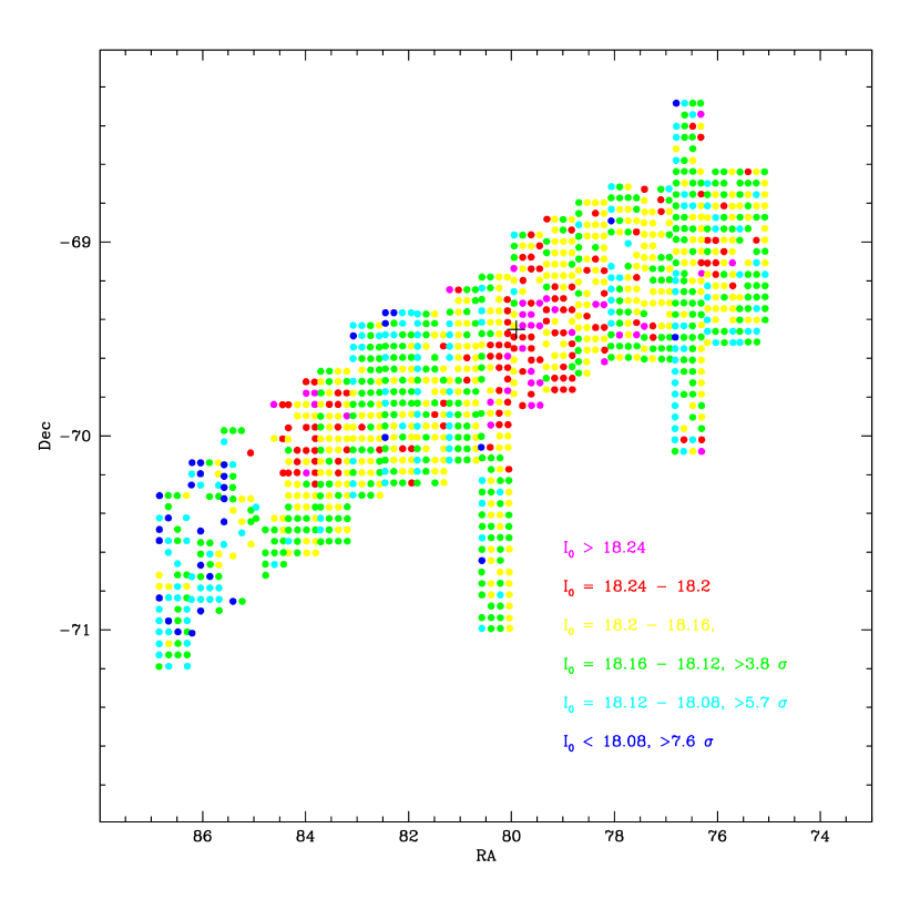
Figure 3: A 2-D plot of the de-reddened mean red clump magnitude, $I_{0}$, for 1123 regions are shown. The colour code used is such that the colour magenta indicates location which are farthest and blue indicates regions which are closest. The statistical significance of the $I_{0}$ bins with respect to maximum random error is also indicated in the figure. The black plus sign shows the location of the LMC center.

The 2D figure of the region studied is shown in figure 3, where the variation in $I_{0}$is shown as a function of RA and Dec. The farthest points have $I_{0}$ more than 18.24 mag and the closest points have $I_{0}$ less than 18.08 mag. This corresponds to a net difference of more than 0.16 mag. This value is more than 7.6 times the maximum random error and more than 5.6 times the maximum total error. Hence the net variation in the de-reddened mean red clump magnitudes is statistically significant.

At locations RA= 79^o.5 and Dec = $-69^{o}$.6 and RA= 84^o.5 and Dec=$-70^{o}$, the $I_{0}$ values are higher indicating that these regions are located at a larger distance. The regions in between the above points are closer to us. The eastern most regions are closest, as indicated in the figure. At RA=84^o.5, another feature which can be noticed is that along the declination axis, there is a change in the relative distance. This is such that the northern regions are farther and the southern regions are closer. The difference in $I_{0}$ is more than 3.8 times the $\Delta_{max}I_{0}$. The center of the LMC is taken to be $05^{h}19^{m}38^{s}.0$ $-69^{o}27^{\prime}5^{\prime\prime}.2$ (2000.0) (de Vaucoulers & Freeman, 1973). Then the center lies near the fainter $I_{0}$ points located around RA=79^o.5. Thus the regions westward of the center are also found to be closer.

In order to study the variation of $I_{0}$ along RA, $I_{0}$ values along declination are averaged, and a plot of avg($I_{0}$) versus RA is shown in figure 4. The error bars indicate the deviation in $I_{0}$ along the declination, for a given RA. It can be seen that there are variations in the $I_{0}$ magnitude along the bar. The center of LMC is shown as an open circle. Most striking feature is the wavy pattern in $I_{0}$. The eastern side of the bar is closer to us, when compared to the bar region near the center. So also is the western side closer to us. We see an M-type variation in $I_{0}$ along the RA. Thus the features indicate that the bar of the LMC is warped. It would be interesting to find the relative inclinations of the disk and the bar, as this will help us estimate their locations. The geometry of the bar based on the $I_{0}$ variation will be presented in another paper, which is in preparation. It would be ideal to use the photometric data of the LMC stars from other surveys, like, MACHO survey to estimate the disk parameters.

The structure of the bar as derived here is delineated by stars belonging to the red clump population. The techniques used in this study are used earlier by many studies (van der Marel, 2001; Udalski et al., 1998; van der Marel & Cioni, 2001). The data used here have been used by Udalski et al. (1998) to estimate distance to the LMC, but they have not used it to study the relative distances within LMC. The reddening is found to be almost a constant along the bar, except in the east end, therefore the magnitude variation is not an imprint of reddening in the bar. The variation in the red clump luminosity could also be due to the age and metallicity difference, rather than due to the relative distance. The study by Subramaniam & Anupama (2002) on the local stellar population of nova regions found no major difference in the population of the intermediate age stars in the Bar region. This is again supported by the findings of Olsen & Salyk (2002) and van der Marel & Cioni (2001). Hence the variation seen in $I_{0}$ magnitude is mainly due to the geometry of the bar. The estimates of self-lensing optical depth in LMC appear to be too low to account fully for the entire microlensing optical depth (Gould, 1995). This kind of a structure in the bar would contribute to more optical depth within LMC, which can increase the self lensing within LMC.

The LMC bar is thus found to show structures. The presence of warp in the bar indicates that the bar is dynamically disturbed. Since the bar is located well within the tidal radius of LMC, the tidal effects due to LMC-SMC-Galaxy interaction may not be the cause of the disturbance. On the other hand, if the bar is not aligned with the disk, then the disk can induce perturbations on the bar. This in turn can create structures in the bar. In order to explain the LMC microlensing events, Zhao & Evans (2000) proposed the bar to be an unvirialised structure, which is slightly mis-aligned with and offset from the LMC disk. Zhao & Evans (2000) also claimed that the interactions of the Magellanic Clouds with the Galaxy could be responsible for the misalignments and displacements of the bar with respect to the disk. Therefore, it is necessary to find out the the geometry of the bar and the disk, which would throw light on the source of perturbations in the bar.

I thank Ram Sagar, Uma Gorti, Anupama and Kiran Jain for helpful discussions. I also thank the referee for his comments which improved the presentation of the paper.

Figure 1: The luminosity function of red clump stars are plotted against I magnitude and (V$-$I) colour. The reduced $\chi^{2}$ value of the fit of the function to the distribution, the estimated values of the peak and its error are indicated in the figure. This data is obtained within a area of 3.56$\times$3.56 arcmin² centered at the location RA = 5^h 32^m 45^s and Dec = $-$70^o 25’ 37”.

Figure 2: Top panel: The error in the estimation of the peak of I magnitude (dots) and (V$-$I) colour (crosses) of the red clump luminosity function are shown as a function of RA for 1191 regions. The dispersion in the reddening E(V$-$I) is indicated as open squares. Bottom panel: The average reddening E(V$-$I) is shown as a function of RA.

Figure 4: The average of the $I_{0}$ along the declination is estimated for various RA and the value avg($I_{0}$) is shown against RA. The error indicates the scatter in $I_{0}$ along the declination. The open circle shows the location of the center of LMC.

References

- de Vaucoulers & Freeman (1973) de Vaucoulers, G., & Freeman, K.C. 1973, Vistas Astron., 14, 163
- Gould (1995) Gould, A., 1995, ApJ, 441, 77
- Olsen & Salyk (2002) Olsen, K.A.G., & Salyk, C. 2002, AJ, 124, 2045
- Schlegel, Finkbeiner & Davis (1998) Schlegel, D.J., Finkbeiner, D.P., & Davis, M. 1998 ApJ, 500, 525
- Subramaniam & Anupama (2002) Subramaniam, A., & Anupama, G.C. 2002, A&A, 390, 449
- Udalski et al. (1998) Udalski, A., Szymanski, M., Kubiak, M., Pietrzynski, G., Wozniak, P., and Zebrun, K. 2000, Acta Astron., 48, 1
- Udalski et al. (2000) Udalski, A., Szymanski, M., Kubiak, M., Pietrzynski, G., Soszynski, I., Wozniak, P., and Zebrun, K. 2000, Acta Astron., 50, 307
- van der Marel (2001) van der Marel, R.P. 2001, AJ, 122, 1827
- van der Marel & Cioni (2001) van der Marel, R.P., & Cioni, M.-R. 2001, AJ, 122, 1807
- Weinberg & Nikolaev (2001) Weinberg, M., & Nikolaev, S. 2001, ApJ, 548, 712
- Zhao & Evans (2000) Zhao, H.S., and Evans, N.W., 2000, ApJ, 545, L35