Unusually Large Fluctuations in the Statistics
of Galaxy Formation at High Redshift

Abstract

We show that various milestones of high-redshift galaxy formation, such as the formation of the first stars or the complete reionization of the intergalactic medium, occurred at different times in different regions of the universe. The predicted spread in redshift, caused by large-scale fluctuations in the number density of galaxies, is at least an order of magnitude larger than previous expectations that argued for a sharp end to reionization. This cosmic scatter in the abundance of galaxies introduces new features that affect the nature of reionization and the expectations for future probes of reionization, and may help explain the present properties of dwarf galaxies in different environments. The predictions can be tested by future numerical simulations and may be verified by upcoming observations. Current simulations, limited to relatively small volumes and periodic boundary conditions, largely omit cosmic scatter and its consequences. In particular, they artificially produce a sudden end to reionization, and they underestimate the number of galaxies by up to an order of magnitude at redshift 20.

1. Introduction

Recent observations of the cosmic microwave background (Spergel et al., 2003) have confirmed the notion that the present large-scale structure in the universe originated from small-amplitude density fluctuations at early cosmic times. Due to the natural instability of gravity, regions that were denser than average collapsed and formed bound halos, first on small spatial scales and later on larger and larger scales. At each snapshot of this cosmic evolution, the abundance of collapsed halos, whose masses are dominated by cold dark matter, can be computed from the initial conditions using numerical simulations and can be understood using approximate analytic models (Press & Schechter, 1974; Bond et al., 1991). The common understanding of galaxy formation is based on the notion that the constituent stars formed out of the gas that cooled and subsequently condensed to high densities in the cores of some of these halos (White & Rees, 1978).

The standard analytic model for the abundance of halos (Press & Schechter, 1974; Bond et al., 1991) considers the small density fluctuations at some early, initial time, and attempts to predict the number of halos that will form at some later time corresponding to a redshift $z$. First, the fluctuations are extrapolated to the present time using the growth rate of linear fluctuations, and then the average density is computed in spheres of various sizes. Whenever the overdensity (i.e., the density perturbation in units of the cosmic mean density) in a sphere rises above a critical threshold $\delta_{c}(z)$, the corresponding region is assumed to have collapsed by redshift $z$, forming a halo out of all the mass that had been included in the initial spherical region. In analyzing the statistics of such regions, the model separates the contribution of large-scale modes from that of small-scale density fluctuations. It predicts that galactic halos will form earlier in regions that are overdense on large scales (Kaiser, 1984; Bardeen et al., 1986; Cole & Kaiser, 1989; Mo & White, 1996), since these regions already start out from an enhanced level of density, and small-scale modes need only supply the remaining perturbation necessary to reach $\delta_{c}(z)$. On the other hand, large-scale voids should contain a reduced number of halos at high redshift. In this way, the analytic model describes the clustering of massive halos.

As gas falls into a dark matter halo, it can fragment into stars only if its virial temperature is above $10^{4}$K for cooling mediated by atomic transitions [or $\sim 500$ K for molecular ${\rm H}_{2}$ cooling; see, e.g., Figure 12 in Barkana & Loeb (2001)]. The abundance of dark matter halos with a virial temperature above this cooling threshold declines sharply with increasing redshift due to the exponential cutoff in the abundance of massive halos at early cosmic times. Consequently, a small change in the collapse threshold of these rare halos, due to mild inhomogeneities on much larger spatial scales, can change the abundance of such halos dramatically. The modulation of galaxy formation by long wavelength modes of density fluctuations is therefore amplified considerably at high redshift. In this paper we show that this results in major new predictions for high-redshift observations. The implications are particularly significant for cosmic reionization and all observational probes of this epoch.

This paper is organized as follows. In § 2 we quantify the scatter in the statistics of galaxy formation produced by this amplification effect. We first explain in § 2.1 the basic physical ideas and implications using the well-established extended Press-Schechter model. We then present in § 2.2 a simple idea that yields a much more accurate model that fits an array of previous simulations at low redshift. We demonstrate the qualitative correctness of our basic assumptions as well as the quantitative accuracy of our model by matching results from recent simulations at high redshift. Since high-redshift galaxies provide the UV photons that lead to the reionization of the intergalactic medium (hereafter IGM), a large scatter is also expected in the reionization redshift within different regions in the universe. We consider this scatter and the modified character of reionization in § 3.1, and show in § 3.2 that existing numerical simulations do not include fluctuations on sufficiently large scales at high redshift. In § 3.3 we discuss the observational implications of the large cosmic scatter expected at high redshift. Finally, we summarize our main results in § 4.

2. Halo Mass Function in Different Environments

2.1. Basic Model: Amplification of Density Fluctuations

Galaxies at high redshift are believed to form in all halos above some minimum mass $M_{\rm min}$ that depends on the efficiency of atomic and molecular transitions that cool the gas within each halo. This makes useful the standard quantity of the collapse fraction $F_{\rm col}(M_{\rm min})$, which is the fraction of mass in a given volume that is contained in halos of individual mass $M_{\rm min}$ or greater. If we set $M_{\rm min}$ to be the minimum halo mass in which efficient cooling processes are triggered, then $F_{\rm col}(M_{\rm min})$ is the fraction of all the baryons in the universe that lie in galaxies. In a large-scale region of comoving radius $R$ with a mean overdensity $\bar{\delta}_{R}$, the standard result is (Bond et al., 1991)

$$F_{\rm col}(M_{\rm min})={\rm erfc}\left[\frac{\delta_{c}(z)-\bar{\delta}_{R}}{\sqrt{2\left[S(R_{\rm min})-S(R)\right]}}\right]\ ,$$ (1)

where $S(R)$ is the variance of fluctuations in spheres of radius $R$, and $S(R_{\rm min})$ is the variance in spheres of radius $R_{\rm min}$ corresponding to the region at the initial time that contained a mass $M_{\rm min}$. In particular, the cosmic mean value of the collapse fraction is obtained in the limit of $R\rightarrow\infty$ by setting $\bar{\delta}_{R}$ and $S(R)$ to zero in this expression. Throughout this section our results assume this standard model, known as the extended Press-Schechter model, which we apply to a universe with cosmological parameters matching the latest observations [specifically, the running index model of Spergel et al. (2003)]. Whenever we consider a cubic region, we estimate its halo abundance by applying the model to a spherical region of equal volume. Note also that we consistently quote values of comoving distance, which equals physical distance times a factor of $(1+z)$.

Our results are based on a simple idea. At high redshift, galactic halos are rare and correspond to high peaks in the Gaussian probability distribution of initial fluctuations. A modest change in the overall density of a large region modulates the threshold for high peaks in the Gaussian density field, so that the number of galaxies is exponentially sensitive to this modulation. This amplification of large-scale modes is responsible for the large statistical fluctuations that we find.

In numerical simulations, periodic boundary conditions are usually assumed, and this forces the mean density of the box to equal the cosmic mean density. The abundance of halos as a function of mass is then biased in such a box (see Figure 1), since a similar region in the real universe will have a distribution of different overdensities $\bar{\delta}_{R}$. At high redshift, when galaxies correspond to high peaks, they are mostly found in regions with an enhanced large-scale density. In a periodic box, therefore, the total number of galaxies is artificially reduced, and the relative abundance of galactic halos with different masses is artificially tilted in favor of lower-mass halos. We illustrate our results for two sets of parameters, one corresponding to the first galaxies and early reionization ($z=20$) and the other to the current horizon in observations of galaxies and late reionization ($z=7$). We consider a resolution equal to that of state-of-the-art cosmological simulations that include gravity and gas hydrodynamics. Specifically, we assume that the total number of dark matter particles in the simulation is $N=324^{3}$, and that the smallest halo that can form a galaxy must be resolved into 500 particles; Springel & Hernquist (2003) showed that this resolution is necessary in order to determine the star formation rate in an individual halo reliably to within a factor of two. Therefore, if we assume that halos that cool via molecular hydrogen must be resolved at $z=20$ (so that $M_{\rm min}=7\times 10^{5}M_{\odot}$), and only those that cool via atomic transitions must be resolved at $z=7$ (so that $M_{\rm min}=10^{8}M_{\odot}$), then the maximum box sizes that can currently be simulated are $l_{\rm box}=1$ Mpc and $l_{\rm box}=6$ Mpc at these two redshifts, respectively.

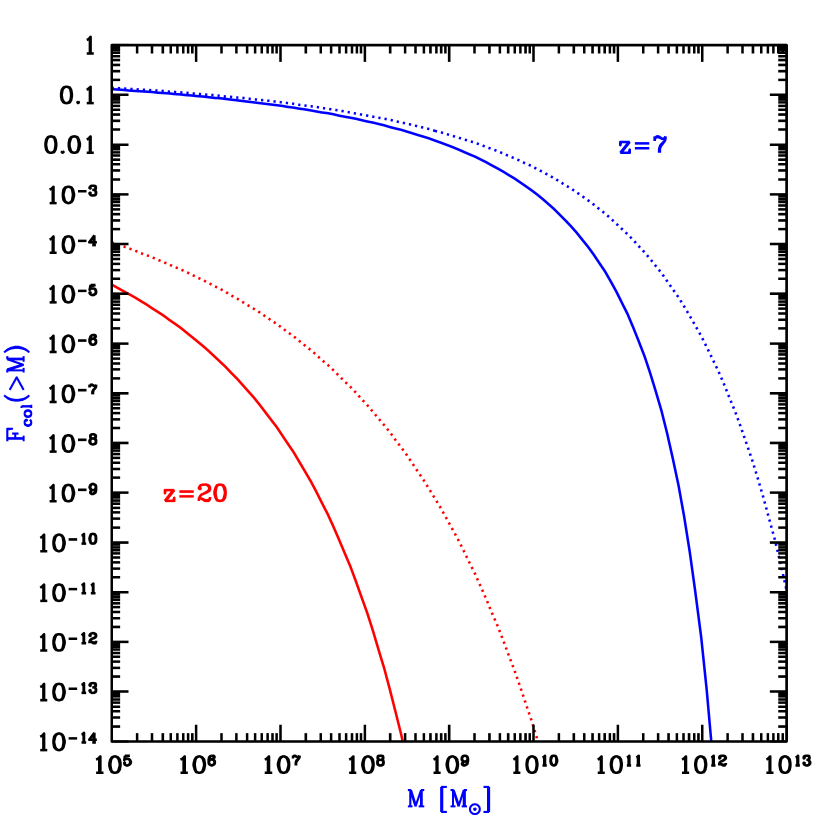
Figure 1.— Bias in the halo mass distribution in simulations. We show the amount of mass contained in all halos of individual mass $M_{\rm min}$ or greater, expressed as a fraction of the total mass in a given volume. This cumulative fraction $F_{\rm col}(M_{\rm min})$ is shown as a function of the minimum halo mass $M_{\rm min}$. We consider two cases of redshift and simulation box size, namely $z=7$, $l_{\rm box}=6$ Mpc (upper curves), and $z=20$, $l_{\rm box}=1$ Mpc (lower curves). At each redshift, we compare the true average distribution in the universe (dotted curve) to the biased distribution (solid curve) that would be measured in a simulation box with periodic boundary conditions (for which $\bar{\delta}_{R}$ is artificially set to zero).

At each redshift we only consider cubic boxes large enough so that the probability of forming a halo on the scale of the entire box is negligible. In this case, $\bar{\delta}_{R}$ is Gaussian distributed with zero mean and variance $S(R)$, since the no-halo condition $\sqrt{S(R)}\ll\delta_{c}(z)$ implies that at redshift $z$ the perturbation on the scale $R$ is still in the linear regime. We can then calculate the probability distribution of collapse fractions in a box of a given size (see Figure 2). This distribution corresponds to a real variation in the fraction of gas in galaxies within different regions of the universe at a given time. In a numerical simulation, the assumption of periodic boundary conditions eliminates the large-scale modes that cause this cosmic scatter. Note that Poisson fluctuations in the number of halos within the box would only add to the scatter, although the variations we have calculated are typically the dominant factor. For instance, in our two standard examples, the mean expected number of halos in the box is 3 at $z=20$ and 900 at $z=7$, resulting in Poisson fluctuations of a factor of about 2 and 1.03, respectively, compared to the clustering-induced scatter of a factor of about 16 and 2 in these two cases.

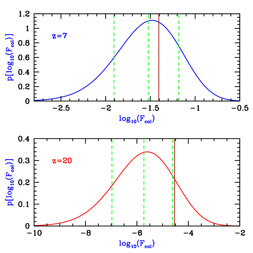
Figure 2.— Probability distribution within a small volume of the total mass fraction in galactic halos. The normalized distribution of the logarithm of this fraction $F_{\rm col}(M_{\rm min})$ is shown for two cases: $z=7$, $l_{\rm box}=6$ Mpc, $M_{\rm min}=10^{8}M_{\odot}$ (upper panel), and $z=20$, $l_{\rm box}=1$ Mpc, $M_{\rm min}=7\times 10^{5}M_{\odot}$ (bottom panel). In each case, the value in a periodic box ($\bar{\delta}_{R}=0$) is shown (central dashed vertical line), along with the value that would be expected given a plus $1-\sigma$ (right dashed line) or a minus $1-\sigma$ (left dashed line) fluctuation in the mean density of the box. Also shown in each case is the mean value of $F_{\rm col}(M_{\rm min})$ averaged over large cosmological volumes (solid vertical line).

Within the extended Press-Schechter model, both the numerical bias and the cosmic scatter can be simply described in terms of a shift in the redshift (see Figure 3). In general, a region of radius $R$ with a mean overdensity $\bar{\delta}_{R}$ will contain a different collapse fraction than the cosmic mean value at a given redshift $z$. However, at some wrong redshift $z+\Delta z$ this small region will contain the cosmic mean collapse fraction at $z$. At high redshifts ($z>3$), this shift in redshift can be easily derived from eq. 1 to be

$$\Delta z=\frac{\bar{\delta}_{R}}{\delta_{0}}-(1+z)\times\left[1-\sqrt{1-\frac{S(R)}{S(R_{\rm min})}}\ \right]\ ,$$ (2)

where $\delta_{0}\equiv\delta_{c}(z)/(1+z)$ is approximately constant at high redshifts (Peebles, 1980), and equals 1.28 for our assumed cosmological parameters. Thus, in our two standard examples, the bias is -2.6 at $z=20$ and -0.4 at $z=7$, and the one-sided $1-\sigma$ scatter is 2.4 at $z=20$ and 1.2 at $z=7$.

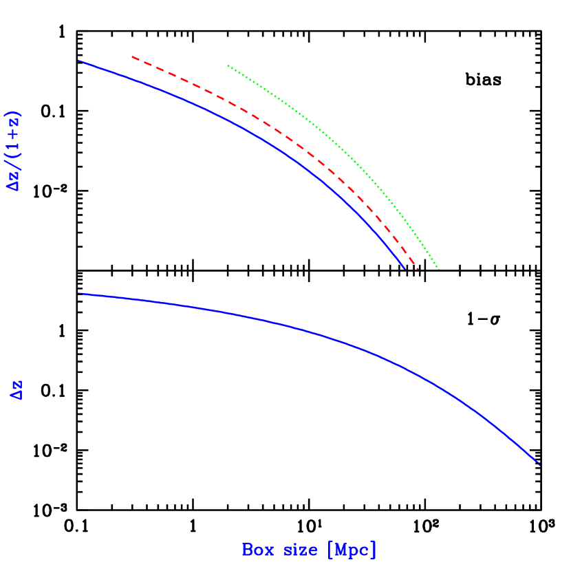
Figure 3.— Cosmic scatter and numerical bias, expressed as the change in redshift needed to get the correct cosmic mean of the collapse fraction. We show the $1-\sigma$ scatter (about the biased value) in the redshift of reionization, or any other phenomenon that depends on the mass fraction in galaxies (bottom panel), as well as the redshift bias [expressed as a fraction of $(1+z)$] in periodic simulation boxes (upper panel). The bias is shown for $M_{\rm min}=7\times 10^{5}M_{\odot}$ (solid curve), $M_{\rm min}=10^{8}M_{\odot}$ (dashed curve), and $M_{\rm min}=3\times 10^{10}M_{\odot}$ (dotted curve). The bias is always negative, and we show its absolute value. When expressed as a shift in redshift, the scatter is independent of $M_{\rm min}$.

2.2. Improved Model: Matching Numerical Simulations

In this subsection we develop an improved model that fits the results of numerical simulations more accurately. The model constructs the halo mass distribution (or mass function); cumulative quantities such as the collapse fraction or the total number of galaxies can then be determined from it via integration. We first define $f(\delta_{c}(z),S)\,dS$ to be the mass fraction contained at $z$ within halos with mass in the range corresponding to $S$ to $S+dS$. The halo abundance is then

$$\frac{dn}{dM}=\frac{\bar{\rho}_{0}}{M}\left|\frac{dS}{dM}\right|f(\delta_{c}(z),S)\ ,$$ (3)

where $dn$ is the comoving number density of halos with masses in the range $M$ to $M+dM$. In the model of Press & Schechter (1974),

$$f_{\rm PS}(\delta_{c}(z),S)=\frac{1}{\sqrt{2\pi}}\frac{\nu}{S}\exp\left[-\frac{\nu^{2}}{2}\right]\ ,$$ (4)

where $\nu=\delta_{c}(z)/\sqrt{S}$ is the number of standard deviations that the critical collapse overdensity represents on the mass scale $M$ corresponding to the variance $S$.

However, the Press-Schechter mass function fits numerical simulations only roughly, and in particular it substantially underestimates the abundance of the rare halos that host galaxies at high redshift. The halo mass function of Sheth & Tormen (1999, see also ) adds two free parameters that allow it to fit numerical simulations much more accurately (Jenkins et al., 2001). We note that these simulations followed very large volumes at low redshift, so that cosmic scatter did not compromise their accuracy. The matching mass function is given by

$$f_{\rm ST}(\delta_{c}(z),S)=A^{\prime}\frac{\nu}{S}\sqrt{\frac{a^{\prime}}{2\pi}}\left[1+\frac{1}{(a^{\prime}\nu^{2})^{q^{\prime}}}\right]\exp\left[-\frac{a^{\prime}\nu^{2}}{2}\right]\ ,$$ (5)

with best-fit parameters (Sheth & Tormen, 2002) $a^{\prime}=0.75$ and $q^{\prime}=0.3$, and where normalization to unity is ensured by taking $A^{\prime}=0.322$.

In order to calculate cosmic scatter we must determine the biased halo mass function in a given volume at a given mean density. Within the extended Press-Schechter model (Bond et al., 1991), the halo mass distribution in a region of comoving radius $R$ with a mean overdensity $\bar{\delta}_{R}$ is given by

$$f_{\rm bias-PS}(\delta_{c}(z),\bar{\delta}_{R},R,S)=f_{\rm PS}(\delta_{c}(z)-\bar{\delta}_{R},S-S(R))\ .$$ (6)

The corresponding collapse fraction in this case is given simply by eq. (1). Despite the relatively low accuracy of the Press-Schechter mass function, the relative change is predicted rather accurately by the extended Press-Schechter model. In other words, the prediction for the halo mass function in a given volume compared to the cosmic mean mass function provides a good fit to numerical simulations over a wide range of parameters (Mo & White, 1996; Casas-Miranda et al., 2002; Sheth & Tormen, 2002).

For our improved model we adopt a hybrid approach that combines various previous models with each applied where it has been found to closely match numerical simulations. We obtain the halo mass function within a restricted volume by starting with the Sheth-Tormen formula for the cosmic mean mass function, and then adjusting it with a relative correction based on the extended Press-Schechter model. In other words, we set

$$f_{\rm bias}(\delta_{c}(z),\bar{\delta}_{R},R,S)=$$

$$f_{\rm ST}(\delta_{c}(z),S)\ \times\left[\frac{f_{\rm PS}(\delta_{c}(z)-\bar{\delta}_{R},S-S(R))}{f_{\rm PS}(\delta_{c}(z),S)}\right]\ .$$ (7)

As noted, this model is based on fits to simulations at low redshifts, but we can check it at high redshifts as well. Figure 4 shows the number of galactic halos at $z\sim 15-30$ in two numerical simulations run by Yoshida et al. (2003), and our predictions given the cosmological input parameters assumed by each simulation. The close fit to the simulated data (with no additional free parameters) suggests that our hybrid model (solid lines) improves on the extended Press-Schechter model (dashed lines), and can be used to calculate accurately the cosmic scatter in the number of galaxies at both high and low redshifts. The simulated data significantly deviate from the expected cosmic mean [eq. (5), shown by the dotted line], due to the artificial suppression of large-scale modes outside the simulated box. We note that Yoshida et al. (2003) mentioned that the lack of large-scale modes might produce a systematically low halo abundance, particularly in the RSI model, but they did not quantify this effect.

Figure 4.— Halo mass function at high redshift in a 1 Mpc box at the cosmic mean density. Our hybrid model prediction (solid lines) is compared with the number of halos above mass $7\times 10^{5}M_{\odot}$ measured in the simulations of Yoshida et al. (2003, data points are taken from their Figure 5). The cosmic mean of the halo mass function (dotted lines) deviates significantly from the simulated values, since the periodic boundary conditions within the finite simulation box artificially set the amplitude of large-scale modes to zero. Our hybrid model starts with the Sheth-Tormen mass function and applies a correction based on the extended Press-Schechter model; in doing so, it provides a better fit to numerical simulations than the pure extended Press-Schechter model (dashed lines) used in the previous figures. We consider two sets of cosmological parameters, the scale-invariant $\Lambda$CDM model of Yoshida et al. (2003) (upper curves), and their running scalar index (RSI) model (lower curves).

As an additional example, we consider the highest-resolution first star simulation (Abel et al., 2002), which used $l_{\rm box}=128$ kpc and $M_{\rm min}=7\times 10^{5}M_{\odot}$. The first star forms within the simulated volume when the first halo of mass $M_{\rm min}$ or larger collapses within the box. To compare with the simulation, we predict the redshift at which the probability of finding at least one halo within the box equals $50\%$, accounting for Poisson fluctuations. We find that if the simulation formed a population of halos corresponding to the correct cosmic average [as given by eq. (5)], then the first star should have formed already at $z=24.0$. The first star actually formed in the simulation box only at $z=18.2$ (Abel et al., 2002). Using eq. (7) we can account for the loss of large-scale modes beyond the periodic box, and predict a first star at $z=17.8$, a close match given the large Poisson fluctuations introduced by considering a single galaxy within the box.

The artificial bias in periodic simulation boxes can also be seen in the results of extensive numerical convergence tests carried out by Springel & Hernquist (2003). They presented a large array of numerical simulations of galaxy formation run in periodic boxes over a wide range of box size, mass resolution, and redshift. In particular, we can identify several pairs of simulations where the simulations in each pair have the same mass resolution but different box sizes; this allows us to separate the effect of large-scale numerical bias from the effect of having poorly-resolved individual halos. Specifically, their simulations Z1 and R4 [see Table 1 in Springel & Hernquist (2003)] used the same particle mass but R4 had a box length larger by a factor of 3.375 . The simulations Q1 and D4 are similarly related, as are Q2 and D5. In each case, the smaller simulation substantially underestimated the star formation rate at high redshift [see Figure 10 in Springel & Hernquist (2003)], Z1 by a factor of 5 at $z=15$ compared to R4, Q1 by a factor of 3 at $z=8$ compared to D4, and Q2 by a factor of 3 at $z=10$ compared to D5.

We note that there have been previous attempts to develop a model for the halo mass function in different environments, so that the model would be consistent with the Sheth-Tormen mass function of eq. (5) which accurately fits the cosmic mean mass function measured in numerical simulations. In order to identify the specific requirements for such a consistency, we first consider the analogous case of the extended Press-Schechter model and its relation to the Press-Schechter formula for the cosmic mean mass function. The extended Press-Schechter model is consistent with the mean mass function in the sense that $f_{\rm bias-PS}$ evaluated for an infinite box (i.e., in the limit where $\bar{\delta}_{R}$ and $S(R)$ both vanish) yields the Press-Schechter mass function:

$$f_{\rm bias-PS}(\delta_{c}(z),0,\infty,S)=f_{\rm PS}(\delta_{c}(z),S)\ .$$ (8)

This condition does not suffice, however, since there is an additional self-consistency test that any viable model must satisfy. Consider any fixed scale $R$. Suppose we consider a very large number $N$ of spheres of radius $R$ within the universe. The mean density $\bar{\delta}_{R}$ in each sphere is determined according to a probability distribution $p(\bar{\delta}_{R})$; we assume that $R$ is large enough so that the probability of forming a halo out of all the mass on the scale $R$ is negligible, and so the distribution is a Gaussian with zero mean and variance $S(R)$ (see also §2.1). The number of galaxies in each sphere is given in the extended Press-Schechter model by eq. (6). As $N\rightarrow\infty$, the halo mass function averaged over all these spheres must approach the cosmic mean value, and it must also approach the ensemble-averaged mass function, where the averaging is performed over the probability distribution of $\bar{\delta}_{R}$. This yields the following self-consistency requirement, which is indeed satisfied by the extended Press-Schechter model:

$$\int f_{\rm bias-PS}(\delta_{c}(z),\bar{\delta}_{R},R,S)\,p(\bar{\delta}_{R})\,d\bar{\delta}_{R}=$$

$$f_{\rm bias-PS}(\delta_{c}(z),0,\infty,S)\ .$$ (9)

Now we again consider attempts to construct an improved model that is consistent with the Sheth-Tormen mass function. Such a model must satisfy eq. (8) (except with $f_{\rm ST}$ on the right-hand side), and it must also satisfy eq. (9) in order to be self-consistent. The latter equation must be satisfied separately for every scale $R$ large enough to avoid collapsing [i.e., that satisfies $\sqrt{S(R)}\ll\delta_{c}(z)$]. Previous proposed models (Sheth & Tormen, 2002; Gottlöber et al., 2003) satisfied simple consistency but not the self-consistency test. Our hybrid model of eq. (7) satisfies both requirements (with respect to the Sheth-Tormen mass function), a result that follows immediately from the fact that the extended Press-Schechter model also satisfies both requirements (with respect to the Press-Schechter mass function). Thus, our hybrid model is the first self-consistent model that is also consistent with the Sheth-Tormen mass function, at least when fluctuations are considered on large scales $R$ for which $\bar{\delta}_{R}$ is Gaussian distributed. As demonstrated in this section, our model also matches results from a wide array of numerical simulations (Abel et al., 2002; Yoshida et al., 2003; Mo & White, 1996; Casas-Miranda et al., 2002; Jenkins et al., 2001).

3. Implications

3.1. The nature of reionization

The photons of the cosmic microwave background have traveled to us mostly undisturbed after neutral atoms first formed in the universe at the cosmic recombination epoch. Radiation from the first generation of stars is thought to have reionized the hydrogen throughout the universe, transforming the IGM back into a hot and highly-ionized plasma.

The popular view developed in the literature (Arons & Wingert, 1972; Fukugita & Kawasaki, 1994; Shapiro et al., 1994; Haiman & Loeb, 1997; Gnedin, 2000; Barkana & Loeb, 2001) maintains that reionization ended with a fast, simultaneous, overlap stage throughout the universe. This view has been based on simple arguments and has been supported by numerical simulations with small box sizes. The underlying idea was that the ionized hydrogen (H II) regions of individual sources began to overlap when the typical size of each H II bubble became comparable to the distance between nearby sources. Since these two length scales were comparable at the critical moment, there is only a single timescale in the problem – given by the growth rate of each bubble – and it determines the transition time between the initial overlap of two or three nearby bubbles, to the final stage where dozens or hundreds of individual sources overlap and produce large ionized regions. Whenever two ionized bubbles were joined, each point inside their common boundary became exposed to ionizing photons from both sources, reducing the neutral hydrogen fraction and allowing ionizing photons to travel farther before being absorbed. Thus, the ionizing intensity inside H II regions rose rapidly, allowing those regions to expand into high-density gas that had previously recombined fast enough to remain neutral when the ionizing intensity had been low. Since each bubble coalescence accelerates the process, it has been thought that the overlap phase has the character of a phase transition and occurs rapidly. Indeed, the best simulations of reionization to date (Gnedin, 2000) found that the average mean free path of ionizing photons in the simulated volume rises by an order of magnitude over a redshift interval $\Delta z=0.05$ at $z=7$.

Our results substantially modify this commonly accepted picture for the development of reionization. Overlap is still expected to occur rapidly, but only in localized high-density regions, where the ionizing intensity and the mean free path rise rapidly even while other distant regions are still mostly neutral. In other words, the size of the bubble of an individual source is about the same in different regions (since most halos have masses just above $M_{\rm min}$), but the typical distance between nearby sources varies widely across the universe. The strong clustering of ionizing sources on length scales as large as 30–100 Mpc introduces long timescales into the reionization phase transition. The sharpness of overlap is determined not by the growth rate of bubbles around individual sources, but by the ability of large groups of sources within overdense regions to deliver ionizing photons into large underdense regions. Simply put, the common view assumes that reionization occurred in patches a few Mpc in size, and that it ended nearly simultaneously in all of them. In reality, however, these two statements are contradictory. If the patches are a few Mpc in size, then there is a very large spread in their reionization redshifts. Conversely, if the spread is small, this implies (from Figure 3) that the patches must be far larger than is commonly assumed.

Note that the recombination rate is higher in overdense regions because of their higher gas density. These regions still reionize first, though, despite the need to overcome the higher recombination rate, since the number of ionizing sources in these regions is increased even more strongly as a result of the dramatic amplification of large-scale modes discussed earlier.

3.2. Limitations of current simulations

The shortcomings of current simulations do not amount simply to a shift of $\sim 10\%$ in redshift and the elimination of scatter, for several reasons. First, the effect that we have identified can be expressed in terms of a shift in redshift only within the context of the extended Press-Schechter model, and only if the total mass fraction in galaxies is considered and not its distribution as a function of galaxy mass. The halo mass distribution should still have the wrong shape, resulting from the fact that $\Delta z$ in eq. 2 depends on $M_{\rm min}$. Furthermore, in our more accurate hybrid model (§ 2.2), the effect on the collapse fraction is no longer exactly equivalent to a shift in redshift. In any case, a self-contained numerical simulation cannot rely on approximate models and must directly evolve a very large volume.

The second reason that current simulations are limited is that at high redshift, when galaxies are still rare, the abundance of galaxies grows rapidly towards lower redshift. Therefore, a $\sim 10\%$ relative error in redshift implies that at any given redshift around $z\sim 10$–20, the simulation predicts a halo mass function that can be off by an order of magnitude for halos that host galaxies (see Figures 1 and 4). This large underestimate suggests that the first generation of galaxies formed significantly earlier than indicated by recent simulations. This makes it easier to explain recent observations of the cosmic microwave background (Spergel et al., 2003) that suggest an early reionization at $z\sim 15$–20.

The third reason for the failure of simulations arises from the large cosmic scatter. This scatter can fundamentally change the character of any observable process or feedback mechanism that depends on a radiation background. Simulations in periodic boxes eliminate any large-scale scatter by assuming that the simulated volume is surrounded by identical periodic copies of itself. In the case of reionization, for instance, current simulations neglect the collective effects described above, whereby groups of sources in overdense regions may influence large surrounding underdense regions. In the case of the formation of the first stars due to molecular hydrogen cooling, the effect of the soft ultraviolet radiation from these stars, which tends to dissociate the molecular hydrogen around them (Haiman et al., 1997; Ricotti et al., 2002; Oh & Haiman, 2003), must be reassessed with cosmic scatter included.

3.3. Observational consequences

The spatial fluctuations that we have calculated fundamentally affect current and future observations that probe reionization or the galaxy population at high redshift. For example, there are a large number of programs searching for galaxies at the highest accessible redshifts (6.5 and beyond) using their strong Ly$\alpha$ emission (Hu et al., 2002; Rhoads et al., 2003; Maier et al., 2003; Kodaira et al., 2003). These programs have previously been justified as a search for the reionization redshift, since the intrinsic emission should be absorbed more strongly by the surrounding IGM if this medium is neutral. For any particular source, it will be hard to clearly recognize this enhanced absorption because of uncertainties regarding the properties of the source and its radiative and gravitational effects on its surroundings (Barkana & Loeb, 2003a, b; Santos, 2003). However, if the luminosity function of galaxies that emit Ly$\alpha$ can be observed, then faint sources, which do not significantly affect their environment, should be very strongly absorbed in the era before reionization. Reionization can then be detected statistically through the sudden jump in the number of faint sources (Haiman & Spaans, 1999; Haiman, 2002). Our results alter the expectation for such observations. Indeed, no sharp “reionization redshift” is expected. Instead, a Ly$\alpha$ luminosity function assembled from a large area of the sky will average over the cosmic scatter of $\Delta z\sim 1$–2 between different regions, resulting in a smooth evolution of the luminosity function over this redshift range. In addition, such a survey may be biased to give a relatively high redshift, since only the most massive galaxies can be detected, and as we have shown, these galaxies will be concentrated in overdense regions that will also get reionized relatively early.

The distribution of ionized patches during reionization will likely be probed by future observations, including small-scale anisotropies of the cosmic microwave background photons that are rescattered by the ionized patches (Aghanim et al., 1996; Gruzinov & Hu, 1998; Santos et al., 2003), and observations of 21 cm emission by the spin-flip transition of the hydrogen in neutral regions (Tozzi et al., 2000; Carilli et al., 2002; Furlanetto et al., 2003). Previous analytical and numerical estimates of these signals have not included the collective effects discussed above, in which rare groups of massive galaxies may reionize large surrounding areas. These photon transfers will likely smooth out the signal even on scales significantly larger than the typical size of an H II bubble due to an individual galaxy. Therefore, even the characteristic angular scales that are expected to show correlations in such observations must be reassessed.

The cosmic scatter also affects observations in the present-day universe that depend on the history of reionization. For instance, photoionization heating suppresses the formation of dwarf galaxies after reionization, suggesting that the smallest galaxies seen today may have formed prior to reionization (Bullock et al., 2001; Somerville, 2002; Benson et al., 2002). Under the popular view that assumed a sharp end to reionization, it was expected that denser regions would have formed more galaxies by the time of reionization, possibly explaining the larger relative abundance of dwarf galaxies observed in galaxy clusters compared to lower-density regions such as our Local Group of galaxies (Tully et al., 2002; Benson et al., 2003a). Our results undercut the basic assumption of this argument and suggest a different explanation altogether. Reionization occurs roughly when the number of ionizing photons produced starts to exceed the number of hydrogen atoms in the surrounding IGM. If the processes of star formation and the production of ionizing photons are equally efficient within galaxies that lie in different regions, then reionization in each region will occur when the collapse fraction reaches the same critical value, even though this will occur at different times in different regions. Since the galaxies responsible for reionization have the same masses as present-day dwarf galaxies, this estimate argues for a roughly equal abundance of dwarf galaxies in all environments today. This simple picture is, however, modified by several additional effects. First, the recombination rate is higher in overdense regions at any given time, as discussed above. Furthermore, reionization in such regions is accomplished at an earlier time when the recombination rate was higher even at the mean cosmic density; therefore, more ionizing photons must be produced in order to compensate for the enhanced recombination rate. These two effects combine to make overdense regions reionize at a higher value of $F_{\rm col}$ than underdense regions. In addition, the overdense regions, which reionize first, subsequently send their extra ionizing photons into the surrounding underdense regions, causing the latter to reionize at an even lower $F_{\rm col}$. Thus, a higher abundance of dwarf galaxies today is indeed expected in the overdense regions.

The same basic effect may be even more critical for understanding the properties of large-scale voids, 10–30 Mpc regions in the present-day universe with an average mass density that is well below the cosmic mean. In order to predict their properties, the first step is to consider the abundance of dark matter halos within them. Numerical simulations show that voids contain a lower relative abundance of rare halos (Cen & Ostriker, 2000; Somerville et al., 2001; Mathis & White, 2002; Benson et al., 2003b), as expected from the raising of the collapse threshold for halos within a void. On the other hand, simulations show that voids actually place a larger fraction of their dark matter content in dwarf halos of mass below $10^{10}M_{\odot}$ (Gottlöber et al., 2003). This can be understood within the extended Press-Schechter model. At the present time, a typical region in the universe fills halos of mass $10^{12}M_{\odot}$ and higher with most of the dark matter, and very little is left over for isolated dwarf halos. Although a large number of dwarf halos may have formed at early times in such a region, the vast majority later merged with other halos, and by the present time they survive only as substructure inside much larger halos. In a void, on the other hand, large halos are rare even today, implying that most of the dwarf halos that formed early within a void can remain as isolated dwarf halos till the present. Thus, most isolated dwarf dark matter halos in the present universe should be found within large-scale voids (Barkana, 2003).

However, voids are observed to be rather deficient in dwarf galaxies as well as in larger galaxies on the scale of the Milky Way (e.g., Kirshner et al., 1981; Eder et al., 1989; Grogin & Geller, 1999, 2000; El-Ad & Piran, 2000; Peebles, 2001). A deficit of large galaxies is naturally expected, since the total mass density in the void is unusually low, and the fraction of this already low density that assembles in large halos is further reduced relative to higher-density regions. The absence of dwarf galaxies is harder to understand, given the higher relative abundance expected for their host dark matter halos. The standard model for galaxy formation may be consistent with the observations if some of the dwarf halos are dark and do not host stars. Large numbers of dark dwarf halos may be produced by the effect of reionization in suppressing the infall of gas into these halos. Indeed, exactly the same factors considered above, in the discussion of dwarf galaxies in clusters compared to those in small groups, apply also to voids. Thus, the voids should reionize last, but since they are most strongly affected by ionizing photons from their surroundings (which have a higher density than the voids themselves), the voids should reionize when the abundance of galaxies within them is relatively low. A quantitative analysis of how the reionization redshift varies with environment may help establish a common framework for explaining the observed properties of dwarf galaxies in environments ranging from clusters to voids.

4. Conclusions

We have shown that the important milestones of high-redshift galaxy formation, such as the formation of the first stars and the completion of reionization, occurred at significantly different times in different regions of the universe. This conclusion results from the fact that the temperature threshold, above which cooling and fragmentation of gas are possible, selects out dark matter halos that become exceptionally rare at high redshifts. Consequently, density fluctuations on large scales modulate the threshold for the collapse of high density peaks on small scales in the exponential tail of the Gaussian random field of density fluctuations, and introduce a remarkably large scatter in the abundance of star-forming galaxies at early cosmic times.

We have developed an improved method to calculate the cosmic scatter (see §2.2). This yields the first self-consistent analytic model that matches the halo mass function measured in various regions in numerical simulations that covered a wide range of the parameter space of region size, mean density, and redshift.

Since the characteristic distance between nearby sources of ionizing radiation varies widely across the universe, the overlap of the H II regions produced by these individual sources in the IGM occurs at significantly different times in different cosmic environments. Quantitatively, we find that the spread in the redshift of reionization should be at least an order of magnitude larger than previous expectations that argued for a sharp end to reionization (see § 3.1).

Current numerical simulations that treat gravity and hydrodynamics (Gnedin, 2000; Abel et al., 2002; Yoshida et al., 2003) largely eliminate this real cosmic scatter, and are artificially biased toward late galaxy formation since they exclude large-scale modes (see Figures 3 and 4). We find that galaxy formation within state-of-the-art simulations with $324^{3}$ particles is artificially biased to occur too late by a redshift interval $\Delta z\sim 0.5$ at $z=7$ and $\Delta z\sim 2.5$ at $z=20$. The box length used in state-of-the-art simulations of reionization (Gnedin, 2000; Yoshida et al., 2003) is 1.5–2 orders of magnitude below the minimum size necessary to treat the scatter reliably, and so alternative computational schemes (Barkana & Loeb, 2003c) must be implemented in order to quantify the implications of the large cosmic scatter on the reionization history. This scatter should affect the statistical fluctuations in the number and clustering properties of sources in surveys with a narrow field of view (such as the Hubble Deep Field), the luminosity function of Ly$\alpha$-emitting galaxies around the reionization redshift, the fluctuations in the 21 cm flux produced by the neutral IGM, the power spectrum of the secondary anisotropies in the cosmic microwave background, and the present abundance of dwarf galaxies in various environments (see § 3.3). Simulations limited to a small box may be able to study the scatter in the number density of galaxies by varying the mean density of the box, but such simulations cannot probe the global structure of reionization since this would involve the radiative transfer of ionizing photons over distances larger than the box size.

References

- Abel et al. (2002) Abel, T., Bryan, G. L., Norman, M. L., Science, 295, 93
- Aghanim et al. (1996) Aghanim, N., Desert, F. X., Puget, J. L., & Gispert, R. 1996, A&A, 311, 1
- Arons & Wingert (1972) Arons, J., & Wingert, D. W. 1972, ApJ, 177, 1
- Bardeen et al. (1986) Bardeen, J. M., Bond, J. R., Kaiser, N., & Szalay, A. S. 1986, ApJ, 304, 15
- Barkana (2003) Barkana, R. 2003, MNRAS, in press (astro-ph/0212458)
- Barkana & Loeb (2001) Barkana, R. & Loeb, A. 2001, Phys. Rep., 349, 125
- Barkana & Loeb (2003a) Barkana, R. & Loeb, A. 2003a, Nature, 421, 341
- Barkana & Loeb (2003b) Barkana, R. & Loeb, A. 2003b, ApJ, in press (preprint astro-ph/0305470)
- Barkana & Loeb (2003c) Barkana, R. & Loeb, A. 2003c, in preparation
- Benson et al. (2003a) Benson, A. J., Frenk, C. S., Baugh, C. M., Cole, S., Lacey, C. G. 2003a, MNRAS, 343, 679
- Benson et al. (2002) Benson, A. J., Frenk, C. S., Lacey, C. G., Baugh, C. M., and Cole, S. 2002, MNRAS, 333, 177
- Benson et al. (2003b) Benson, A. J., Hoyle, F., Torres, F., & Vogeley, M. S. 2003b, MNRAS, 340, 160
- Bond et al. (1991) Bond, J. R., Cole, S., Efstathiou, G., & Kaiser, N. 1991, ApJ, 379, 440
- Bullock et al. (2001) Bullock, J. S., Kravtsov, A. V., & Weinberg, D. H. 2001, ApJ, 548, 33
- Carilli et al. (2002) Carilli, C. L., Gnedin, N. Y., & Owen, F. 2002, ApJ, 577, 22
- Casas-Miranda et al. (2002) Casas-Miranda, R., Mo, H. J., Sheth, R. K., Börner, G. 2002, MNRAS, 333, 730
- Cen & Ostriker (2000) Cen, R. & Ostriker, J. P. 2000, ApJ, 538, 83
- Ciardi, Stoehr, & White (2003) Ciardi, B., Stoehr, F., & White, S. D. M. 2003, MNRAS, 343, 1101
- Cole & Kaiser (1989) Cole, S., & Kaiser, N. 1989, MNRAS, 237, 1127
- Eder et al. (1989) Eder, J., Oemler, A. J., Schombert, J. M., & Dekel, A. 1989, ApJ, 340, 29
- El-Ad & Piran (2000) El-Ad, H. & Piran, T. 2000, MNRAS, 313, 553
- Fukugita & Kawasaki (1994) Fukugita, M., & Kawasaki, M. 1994, MNRAS, 269, 563
- Furlanetto et al. (2003) Furlanetto, S., Sokasian, A., & Hernquist, L. 2003, MNRAS, in press (preprint astro-ph/0305065)
- Gnedin (2000) Gnedin, N. Y. 2000, ApJ, 535, 530
- Gottlöber et al. (2003) Gottlöber, S., Łokas, E. L., Klypin, A., & Hoffman, Y. 2003, MNRAS, 344, 715
- Grogin & Geller (1999) Grogin, N. A. & Geller, M. J. 1999, AJ, 118, 2561
- Grogin & Geller (2000) Grogin, N. A. & Geller, M. J. 2000, AJ, 119, 32
- Gruzinov & Hu (1998) Gruzinov, A., & Hu, W. 1998, ApJ, 508, 435
- Haiman (2002) Haiman, Z. 2002, ApJ, 576, L1
- Haiman & Loeb (1997) Haiman, Z., & Loeb, A. 1997, ApJ, 483, 21; erratum – 1998, ApJ, 499, 520
- Haiman et al. (1997) Haiman, Z., Rees, M. J., & Loeb, A. 1997, ApJ, 476, 458; erratum, 484, 985
- Haiman & Spaans (1999) Haiman, Z. & Spaans, M. 1999, ApJ, 518, 138
- Hu et al. (2002) Hu, E. M., et al. 2002, ApJ, 568, 75; erratum, 576, 99
- Jenkins et al. (2001) Jenkins, A., et al. 2001, MNRAS, 321, 372
- Kaiser (1984) Kaiser, N. 1984, ApJ, 284, L9
- Kirshner et al. (1981) Kirshner, R. P., Oemler, A., Schechter, P. L., & Shectman, S. A. 1981, ApJ, 248, L57
- Kodaira et al. (2003) Kodaira, K., et al. 2003, PASJ, 55, 2, L17
- Maier et al. (2003) Maier, C., et al. 2003, A&A, 402, 79
- Mathis & White (2002) Mathis, H. & White, S. D. M. 2002, MNRAS, 337, 1193
- Mo & White (1996) Mo, H. J. & White, S. D. M. 1996, MNRAS, 282, 347
- Oh & Haiman (2003) Oh, S. P., & Haiman, Z. 2003, MNRAS, in press (preprint astro-ph/0307135)
- Peebles (1980) Peebles, P. J. E. 1980, The Large-Scale Structure of the Universe (Princeton: PUP)
- Peebles (2001) Peebles, P. J. E. 2001, ApJ, 557, 495
- Press & Schechter (1974) Press, W. H., & Schechter, P. 1974, ApJ, 187, 425
- Ricotti et al. (2002) Ricotti, M., Gnedin, N. Y., & Shull, M. J. 2002, ApJ, 575, 49
- Rhoads et al. (2003) Rhoads, J. E., et al. 2003, AJ, 125, 1006
- Santos (2003) Santos, M. R. 2003, MNRAS, in press (preprint astro-ph/0308196).
- Santos et al. (2003) Santos, M. G., Cooray, A., Haiman, Z., Know, L., & Ma, C.-P. 2003, ApJ, in press (preprint astro-ph/0305471)
- Shapiro et al. (1994) Shapiro, P. R., Giroux, M. L., & Babul, A. 1994, ApJ, 427, 25
- Sheth et al. (2001) Sheth, R. K., Mo, H. J., & Tormen, G. 2001, MNRAS, 323, 1
- Sheth & Tormen (1999) Sheth, R. K., & Tormen, G. 1999, MNRAS, 308, 119
- Sheth & Tormen (2002) Sheth, R. K., & Tormen, G. 2002, MNRAS, 329, 61
- Somerville et al. (2001) Somerville, R. S., Lemson, G., Sigad, Y., Dekel, A., Kauffmann, G., & White, S. D. M. 2001, MNRAS, 320, 289
- Somerville (2002) Somerville, R. S. 2002, ApJ, 572, L23
- Spergel et al. (2003) Spergel, D. N., et al. 2003, ApJS, 148, 175
- Springel & Hernquist (2003) Springel, V., & Hernquist, L. 2003, MNRAS, 339, 312
- Tozzi et al. (2000) Tozzi, P., Madau, P., Meiksin, A., & Rees, M. J. 2000, ApJ, 528, 597
- Tully et al. (2002) Tully, R. B., Somerville, R. S., Trentham, N., & Verheijen, M. A. W. 2002, ApJ, 569, 573
- Yoshida et al. (2003) Yoshida, N., Sokasian, A., Hernquist, L., & Springel, V. 2003, ApJ, in press (astro-ph/0305517)
- White & Rees (1978) White, S. D. M., & Rees, M. J. 1978, MNRAS, 183, 341