Quasi-Local Evolution of the Cosmic Gravitational Clustering in Halo Model

Abstract

We show that the nonlinear evolution of the cosmic gravitational clustering is approximately spatial local in the $x$-$k$ (position-scale) phase space if the initial perturbations are Gaussian. That is, if viewing the mass field with modes in the phase space, the nonlinear evolution will cause strong coupling among modes with different scale $k$, but at the same spatial area $x$, while the modes at different area $x$ remain uncorrelated, or very weakly correlated. We first study the quasi-local clustering behavior with the halo model, and demonstrate that the quasi-local evolution in the phase space is essentially due to the self-similar and hierarchical features of the cosmic gravitational clustering. The scaling of mass density profile of halos insures that the coupling between $(x-k)$ modes at different physical positions is substantially suppressed. Using high resolution N-body simulation samples in the LCDM model, we justify the quasi-locality with the correlation function between the DWT (discrete wavelet transform) variables of the cosmic mass field. Although the mass field underwent a highly non-linear evolution, and the DWT variables display significantly non-Gaussian features, there are almost no correlations among the DWT variables at different spatial positions. Possible applications of the quasi-locality have been discussed.

1 Introduction

The large scale structure of the universe was arisen from initial fluctuations through the nonlinear evolution of gravitational instability. Gravitational interaction is of long range, and therefore, the evolution of cosmic clustering is not localized in physical space. The typical processes of cosmic clustering, such as collapsing and falling into potential wells, the Fourier mode-mode coupling and the merging of pre-virialized dark halos, are generally non-local. These processes lead to a correlation between the density perturbations at different positions, even if the perturbations at that positions initially are statistically uncorrelated. For instance, in the Zel’dovich approximation (Zel’dovich 1970), the density field $\rho({\bf x},t)$ at (Eulerian) comoving position ${\bf x}$ and time $t$ is determined by the initial perturbation at (Lagrangian) comoving position, ${\bf q}$, plus a displacement ${\bf S}$:

$${\bf x}({\bf q},t)={\bf q}+{\bf S}({\bf q},t).$$ (1)

The displacement ${\bf S}({\bf q},t)$ represents the effect of density perturbations on the trajectories of self-gravitating particles. The intersection of particle trajectories leads to a correlation between mass fields at different spatial positions. Thus, the gravitational clustering is non-local even in weakly non-linear regime.

On the other hand, spatial locality has been employed in the Gaussianization technique for recovery of the primordial power spectrum (Narayanan & Weinberg 1998). Underlying this algorithm is to assume that the relation between the evolved mass field and the initial density distribution is local, i.e. the high(low) initial density pixels will be mapped into high(low) density pixels of the evolved field (Narayanan & Weinberg 1998). Obviously, the localized mapping is difficult in reconciling the initially Gaussian field with the coherent non-linear structures, such as halos with scaling behavior. It has been argued that the locality assumption may be a poor approximation to the actual dynamics because of the non-locality of gravitational evolution (Monaco & Efstathiou 2000). Nevertheless, the localized mapping is found to work well for reconstructing the initial mass field and power spectrum from transmitted flux of the Ly$\alpha$ absorption in QSO spectra (Croft et al. 1998.) These results, joint with the data of WMAP, have been used to determine the cosmological parameters (Spergel et al 2003). However, the dynamical origin of the locality assumption remains a problem. It is still unclear under which condition the localized mapping is a good approximation.

This problem has been studied in weakly non-linear regime under the Zel’dovich approximation. The result showed that the cosmic gravitational clustering evolution is spatially quasi-localized in phase ($x$-$k$) space made by the DWT decomposition (Pando, Feng & Fang 2001). In this approach, each perturbation mode corresponds to a cell in the $x$-$k$ space, ($x$ to $x+\Delta x$, $k$ to $k+\Delta k$) with $\Delta x\Delta k=2\pi$, and the density perturbation of the mode $(x,k)$ is $\delta(k,x)$. They demonstrated that, in the Zel’dovich approximation, if the initial density perturbations in each cells are statistically uncorrelated, i.e. $\langle\delta_{0}(k_{1},x_{1})\delta_{0}(k_{2},x_{2})\rangle\propto\delta^{K}_{k_{1},k_{2}}\delta^{K}_{x_{1}.x_{2}}$, where $\delta^{K}$ denotes for Kronecker delta function, the evolved $\delta(k_{1},x_{1})$ and $\delta(k_{2},x_{2})$ will keep approximately spatially uncorrelated always, $\langle\delta(k_{1},x_{1})\delta(k_{2},x_{2})\rangle\propto\delta^{K}_{x_{1}.x_{2}}$, which is just what we call spatial quasi-locality in the dynamics of cosmic clustering. The spatial quasi-locality implies a significant local mode-mode coupling (different scales $k$ at the same position $x$), but very weak non-local coupling between the modes (different positions $x$). The non-linear dynamical evolution is well developed along the direction of ${\bf k}$-axis, rather than ${\bf x}$-axis in the phase space. This quasi-locality has been justified in weak nonlinear samples such as the transmitted flux of QSO Ly$\alpha$ absorption spectrum (Pando, Feng & Fang 2001). It places the dynamical base of recovering initial power spectrum from corresponding weakly evolved field via a localized mapping in phase space (Feng & Fang 2000).

This paper is to extend the concept of quasi-locality to fully nonlinear regime. We try to show that the quasi-locality of the cosmic clustering in phase space holds not only in the weak nonlinear regime, but also in nonlinear evolution. Since the nonlinear cosmic density field can be expressed by the semianalytical halo model (e.g. Cooray & Sheth 2002, and references therein), our primary interest is to study whether the quasi-locality could be incorporated in the halo model. We will first analytically derive the quasi-locality from the halo model, and then make a numerical test using high resolution $N$-body simulation samples.

The outline of this paper is as follows. §2 presents the statistical criterion of the quasi-local evolution of a density clustering in the $x$-$k$ phase space. §3 shows that the density field evolution might be spatially quasi-localized in the phase space if the cosmic density field can be described by the halo model. Numerical tests on these predictions with N-body simulation samples are made in §4. Finally, the conclusions and discussions will be given in §5.

2 Quasi-Locality in $x$-$k$ Space

2.1 DWT Variables of the Mass Field

In physical space (${\bf x}$), the mode is Dirac delta function $\delta^{D}({\bf x})$, and cosmic mass density field variable is $\rho({\bf x})$, while in scale space (${\bf k}$), the mode is the Fourier bases $e^{i{\bf k}\cdot{\bf x}}$, and the field variable is $\hat{\rho}({\bf k})$, which is the Fourier transform of $\rho({\bf x})$. In hybrid $x$-$k$ phase space, one can use the complete and orthogonal bases of the discrete wavelet transform (DWT) as the mode function. The mass density field is then described by the DWT variables.

Without loss of generality, we introduce the DWT variables by considering a density field $\rho({\bf x})$ in a cubic box of $0\leq x^{i}\leq L$, $i=1,2,3$ and volume $V=L^{3}$. We first divide the box into cells with volume $L^{3}/2^{j_{1}+j_{2}+j_{3}}$, where $j_{1},j_{2},j_{3}=0,1...$. For a given ${\bf j}\equiv(j_{1},j_{2},j_{3})$, there are $2^{j_{1}+j_{2}+j_{3}}$ cells labelled by ${\bf l}\equiv(l_{1},l_{2},l_{3})$, and $l_{i}=0,1...2^{j_{i}}-1$. The cell $(l_{1},l_{2},l_{3})$ occupies the spatial range $lL/2^{j_{i}}<x_{i}\leq(l+1)L/2^{j_{i}}$, $i=1,2,3$. Accordingly, indexes ${\bf j}$ and ${\bf l}$ denote for, respectively, the scale and the position of the cells. In each dimension, we have $\Delta x_{i}=L/2^{j_{i}}$ and $\Delta k_{i}=2\pi/(L/2^{j})$, i.e. $\Delta x_{i}\Delta k=2\pi$, or the volume of all cells in the $x$-$k$ space is $(2\pi)^{3}$.

Each cell $({\bf j,l})$ supports two compact functions: the scaling function $\phi_{\bf j,l}({\bf x})$ and the wavelets $\psi_{\bf j,l}({\bf x})$ (Daubechies 1992, Fang & Thews, 1998, Fang & Feng, 2000). Both $\phi_{\bf j,l}({\bf x})$ and $\psi_{\bf j,l}({\bf x})$ are localized in cell (${\bf j,l}$). The scaling functions $\phi_{\bf j,l}({\bf x})$ are orthogonormal with respect to index ${\bf l}$ as

$$\int\phi_{\bf j,l}({\bf x})\phi_{\bf j,l^{\prime}}({\bf x})d{\bf x}=\delta_{\bf l,l^{\prime}}.$$ (2)

The scaling function $\phi_{\bf j,l}({\bf x})$ is a low pass filter at cell $({\bf j,l})$. The scaling function coefficient (SFC) of the density field is defined by

$$\epsilon_{\bf j,l}=\int\rho({\bf x})\phi_{\bf j,l}({\bf x})d{\bf x},$$ (3)

which is proportional to the mean density in cell $({\bf j,l})$.

The wavelets $\psi_{\bf j,l}({\bf x})$ are orthogonormal with respect to both indexes ${\bf j}$ and ${\bf l}$

$$\int\psi_{\bf j,l}({\bf x})\psi_{\bf j^{\prime},l^{\prime}}({\bf x})d{\bf x}=\delta_{\bf j,j^{\prime}}\delta_{\bf l,l^{\prime}}.$$ (4)

The wavelets $\{\psi_{\bf j,l}({\bf x})\}$ form a complete and orthogonal base (mode) in the phase space. Therefore, the density field can be described by the wavelet function coefficients (WFCs) defined as

$$\tilde{\epsilon}_{\bf j,l}=\int d{\bf x}\rho({\bf x})\psi_{\bf j,l}({\bf x}).$$ (5)

The WFCs $\tilde{\epsilon}_{\bf j,l}$ are the DWT variables of the density field. The DWT variables $\tilde{\epsilon}_{\bf j,l}$ is the fluctuation of the density field around scales ${\bf k}=2\pi{\bf n}/L$, ${\bf n}=(2^{j_{1}},2^{j_{2}},2^{j_{3}})$ located at the cell ${\bf l}$ with size $\Delta{\bf x}=(L/2^{j_{1}},L/2^{j_{2}},L/2^{j_{3}})$. Since the wavelet $\psi_{\bf j,l}({\bf x})$ is a band pass filter, in each dimension, $\tilde{\epsilon}_{\bf j,l}$ is a superposition of fluctuations filtered in the waveband $k\pm\Delta k/2$, where $k=2\pi 2^{j}/L$, and $\Delta k=2\pi/\Delta x=k$. This decomposition of the fluctuation is optimized in sense that the size of cell $\Delta x$ is adaptively chosen to match with the perturbations at a given wavenumber.

The DWT bases generally have vanishing moments, i.e.

$$\int x^{t}\psi_{\bf j,l}({\bf x})d{\bf x}=0,$$ (6)

where $t=0,1...M-1$ and $M\geq 1$. $M$ is dependent on wavelet. For the wavelet Daubechies $2n$, we have $M=n$. Thus, the Fourier transform of wavelet $\hat{\psi}_{\bf j,l}({\bf k})=\int\psi_{\bf j,l}({\bf x})\exp(-i{\bf k}\cdot{\bf x})d{\bf x}$ has a compact support in the wavenumber space $\{{\bf k}\}$. From eq.(6) we have $\int\bar{\rho}\psi_{\bf j,l}({\bf x})d{\bf x}=0$ for all ${\bf j,l}$, and thus,

$$\tilde{\epsilon}_{\bf j,l}=\bar{\rho}\int d{\bf x}\delta({\bf x})\psi_{\bf j,l}({\bf x})$$ (7)

where the density contrast $\delta({\bf x})=[\rho({\bf x})-\bar{\rho}]/\bar{\rho}$, $\bar{\rho}$ is the mean density. Since $\langle\delta({\bf x})\rangle=0$, we have also

$$\langle\tilde{\epsilon}_{\bf j,l}\rangle=0$$ (8)

Because the set of wavelets is complete, $\tilde{\epsilon}_{\bf j,l}$ give a complete description of the density field $\rho({\bf x})$, i.e. one can reconstruct $\rho({\bf x})$ or $\delta({\bf x})$ in terms of variables $\tilde{\epsilon}_{\bf j,l}$ as

$$\delta({\bf x})=\frac{1}{\bar{\rho}}\sum_{\bf j,l}\tilde{\epsilon}_{\bf j,l}\psi_{\bf j,l}({\bf x}).$$ (9)

2.2 Quasi-Locality of Gaussian Fields

The initial density perturbation of the universe $\delta({\bf x},t_{i})$ is believed to be a Gaussian random field with correlation matrix of the Fourier variables $\hat{\delta}({\bf k},t_{i})$

$$\langle\hat{\delta}({\bf k},t_{i})\hat{\delta}({\bf k^{\prime}},t_{i})\rangle=P({\bf k},t_{i})\delta^{K}_{\bf k,-k^{\prime}},$$ (10)

and all higher order cumulant moments of $\hat{\delta}({\bf k},t_{i})$ vanish. The function $P({\bf k},t_{i})$ of eq.(10) is the initial power spectrum. The Kronecker delta function $\delta^{K}_{\bf k,k^{\prime}}$ in eq.(10) indicates that the initial perturbation for each mode ${\bf k}$ is independent, or localized in $k$-space.

Generally, if the initial Fourier power spectrum, $P({\bf k},t_{i})$, is colored, i.e. $k$-dependent, the correlation matrix of variables other than the Fourier mode will no longer be diagonal. For instance, correlation function in $x$-space will be $\langle\delta({\bf x},t_{i})\delta({\bf x^{\prime}},t_{i})\rangle=\xi({\bf|x-x|}^{\prime},t_{i})$, which is the Fourier counterpart of $P({\bf k},t_{i})$. However, the correlation matrix of the DWT variables of a Gaussian field is always diagonal or quasi-diagonal, regardless the Fourier power spectrum $P(k)$ is white or colored. That is, the correlation function of $\tilde{\epsilon}_{\bf j,l}$ is localized with respect to $({\bf j,l})$ as

$$\langle\tilde{\epsilon}_{\bf j,l}(t_{i})\tilde{\epsilon}_{\bf j^{\prime},l^{\prime}}(t_{i})\rangle\simeq P_{\bf j,l}(t_{i})\delta^{K}_{\bf j,j^{\prime}}\delta^{K}_{\bf l,l^{\prime}},$$ (11)

where $P_{\bf j,l}$ in eq.(11) is the DWT power spectrum of the field.

The reason of the diagonality of eq.(11) is as follows. First, the WFC $\tilde{\epsilon}_{\bf j,l}$ is given by a linear superposition of the Fourier modes $\hat{\delta}({\bf k})$ in the waveband around $k_{i}\simeq 2\pi 2^{j_{i}}/L$ ($i=1,2,3$), $\tilde{\epsilon}_{\bf j,l}$ with different ${\bf j}$ consist of the Fourier modes $\hat{\delta}({\bf k})$ in different ${\bf k}$ bands. While for Gaussian fields, the Fourier modes in different wave bands are uncorrelated in general [eq.(10)], and therefore, there might be no correlation between the DWT modes of ${\bf j}$ and ${\bf j^{\prime}}$ if ${\bf j\neq j^{\prime}}$. This yields the quasi-locality of $\delta^{K}_{\bf j,j^{\prime}}$. Second, the phases of the Fourier modes of Gaussian field are independent and random. For a superposition of the random phased Fourier modes $\hat{\delta}({\bf k})$ in the band from ${\bf k}$ to ${\bf k+\Delta k}$, the spatial correlation length can not be larger than that given by the uncertainty relation $\Delta x\simeq 2\pi/\Delta k\simeq 2^{-j}L$. Moreover, the non-zero regions of two DWT modes $\psi_{\bf j,l}$ and $\psi_{\bf j,l^{\prime}}$ with $({\bf l\neq l^{\prime}})$ have spatial distance $\Delta|x_{i}|\simeq 2^{-j_{i}}L|l_{i}-l^{\prime}_{i}|$. Consequently, all off-diagonal elements $({\bf l\neq l^{\prime}})$ vanish or are much smaller than diagonal elements, i.e.,

$$\frac{|\int d{\bf x}\int d{\bf x^{\prime}}\psi_{\bf j,l}({\bf x})\xi({\bf x-x^{\prime}},t_{i})\psi_{\bf j^{\prime},l^{\prime}}({\bf x^{\prime}})|}{\int d{\bf x}\int d{\bf x^{\prime}}\psi_{\bf j,l}({\bf x})\xi({\bf x-x^{\prime}},t_{i})\psi_{\bf j,l}({\bf x^{\prime}})}\ll 1,\hskip 14.22636pt{\rm if\ \ }{\bf l}\neq{\bf l^{\prime}}\hskip 5.69054pt{\rm or\ \ }{\bf j}\neq{\bf j^{\prime}}.$$ (12)

Thus, the correlation function of the DWT variables of a Gaussian field is rapidly decaying when $|{\bf l-l^{\prime}}|\geq 1$ and $|{\bf j-j^{\prime}}|\geq 1$. The diagonal correlation function described by eq.(11) is a generic feature of a Gaussian field in the DWT representation.

It should be pointed out that the WFC correlation function eq.(11) is different from the ordinary two point correlation function $\langle\delta({\bf x})\delta({\bf x^{\prime}})\rangle=\xi({\bf x,x^{\prime}})$. The former is the correlation between two modes in $(x-k)$ phase space, while the later is for two modes in $x$-space. Explicitly, eq.(11) describes the correlation of perturbation modes in the waveband $k\rightarrow k+\Delta k$ between positions ${\bf l}$ and ${\bf l^{\prime}}$, and so, it is sensitive to the phases of modes. The ordinary two point correlation is not sensitive to the phase of perturbations. In the DWT analysis, an analogue of the ordinary two point correlation function is defined by by the correlation between SFCs, i.e. $\langle\epsilon_{\bf j,l}(t_{i})\epsilon_{\bf j^{\prime},l^{\prime}}(t_{i})\rangle$. Since the scaling function $\phi_{\bf j,l}$ is a low-pass filter on scale ${\bf j}$ and at position ${\bf l}$, the correlation function $\langle\epsilon_{\bf j,l}(t_{i})\epsilon_{\bf j^{\prime},l^{\prime}}(t_{i})\rangle$ behaves in a similar way as $\langle\delta_{R}({\bf x})\delta_{R}({\bf x^{\prime}})\rangle$, where $\delta_{R}({\bf x})$ is a filtered density field smoothed on the scale $R\sim 2^{-j}L$. However, as $\psi_{\bf j,l}$ is a high-pass filter, the WFC covariance $\langle\tilde{\epsilon}_{\bf j,l}\tilde{\epsilon}_{\bf j^{\prime},l^{\prime}}\rangle$ shows quite different statistical features from the SFC correlation, e.g., it is always quasi-diagonal or even fully diagonal for a Gaussian field. Generally, it has been shown for many analytically calculable random fields that the SFC correlation is significantly off-diagonal, while the WFC correlation is exactly diagonal (Greiner, Lip & Carruthers, 1995)

Moreover, within a given volume in the $x$-$k$ space, such as $Vd^{3}{\bf k}$, the number of the DWT modes $\{\bf j,l\}$ is the same as that of the Fourier modes ${\bf k}$. Accordingly, $P({\bf k},t_{i})$ can be expressed as a linear superposition of $P_{\bf j,l}(t_{i})$, and vice versa. Equivalently, the Fourier power spectrum can be replaced by the DWT power spectrum (Fang & Feng, 2000).

2.3 Statistical Criterions of Quasi-Locality

If the evolution of the comic mass field is localized, the evolved density field $\delta({\bf x})$ at a given spatial point is determined only by the initial density distribution $\delta({\bf x},t_{i})$ at the same point. As emphasized in §1, this locality is inconsistent with the non-local behavior of gravitational clustering. However, the evolution of the comic mass field can be quasi-localized in sense that the correlation between the DWT variables of the evolved field is always spatial diagonal if the initial correlation function is diagonal, such as eq.(11). For perturbation modes in a waveband $k\rightarrow k+\Delta k$, the quasi-localized range is $\Delta x\simeq 2\pi/\Delta k$.

A quasi-localized evolution means that the auto-correlation function of the DWT variables is always diagonal, or quasi-diagonal $\langle\tilde{\epsilon}_{\bf j,l}\tilde{\epsilon}_{\bf j^{\prime},l^{\prime}}\rangle\ll\langle\tilde{\epsilon}_{\bf j,l}\tilde{\epsilon}_{\bf j^{\prime},l}\rangle$ when ${\bf l\neq l^{\prime}}$, if it is diagonal initially. Thus, one may place a statistical criterion for the quasi-locality as

$$\kappa_{\bf j,j^{\prime}}(\Delta{\bf l})\ll 1,\ \ {\rm\ if\ }\Delta{\bf l}\neq 0,$$ (13)

where

$$\kappa_{\bf j,j^{\prime}}(\Delta{\bf l})=\frac{\langle\tilde{\epsilon}_{\bf j,l}\tilde{\epsilon}_{\bf j^{\prime},l^{\prime}}\rangle}{\langle|\tilde{\epsilon}_{\bf j,l}|^{2}\rangle^{1/2}\langle|\tilde{\epsilon}_{\bf j^{\prime},l^{\prime}}|^{2}\rangle^{1/2}}.$$ (14)

This is a normalized correlation function of the DWT modes, i.e. $\kappa_{\bf j,j}(\Delta{\bf l}=0)=1$.

The auto-correlation function of the DWT variables, $\langle\tilde{\epsilon}_{\bf j,l}\tilde{\epsilon}_{\bf j^{\prime},l^{\prime}}\rangle$, measures the correlations between the perturbation modes on scales ${\bf j}=(j_{1},j_{2},j_{3})$ and ${\bf j^{\prime}}=(j_{1}^{\prime},j_{2}^{\prime},j_{3}^{\prime})$ at two cells with a vector distance given by $(l_{1}L/2^{j_{1}}-l_{1}^{\prime}L/2^{j_{1}^{\prime}},l_{2}L/2^{j_{2}}-l_{2}^{\prime}L/2^{j_{2}^{\prime}},l_{3}L/2^{j_{3}}-l_{3}^{\prime}L/2^{j_{3}^{\prime}})$. In the case of $\Delta l=0$, $\kappa_{\bf j,j^{\prime}}(0)$ gives the correlation between fluctuations on scale $j$ and $j^{\prime}$ at the same physical area. Therefore, if condition (13) holds for all redshifts, the dynamical evolution of the mass field is basically spatial localized in the DWT bases. Comparing the condition eq.(13) with eq.(12), we see that the cosmic field undergoing a local evolution is different from its Gaussian predecessor by the factor $\delta^{K}_{\bf j,j^{\prime}}$, but not $\delta^{K}_{\bf l,l^{\prime}}$. In other words, the evolution leads to the significant scale-scale $({\bf j,j^{\prime}})$ coupling, rather than modes at different locations ${\bf l\neq l^{\prime}}$.

One can also construct the criterions for the quasi-locality using higher order correlations among the DWT variables $\tilde{\epsilon}_{\bf j,l}$. For instance, a $(p+q)$ order statistical criterion is given by

$$C^{p,q}_{\bf j,j^{\prime}}(\Delta{\bf l}\neq 0)\simeq 1.$$ (15)

where

$$C^{p,q}_{\bf j,j^{\prime}}(\Delta{\bf l})=\frac{\langle\tilde{\epsilon}^{p}_{\bf j,l}\tilde{\epsilon}^{q}_{\bf j^{\prime},l^{\prime}}\rangle}{\langle\tilde{\epsilon}^{p}_{\bf j,l}\rangle\langle\tilde{\epsilon}^{q}_{\bf j^{\prime},l^{\prime}}\rangle},$$ (16)

where $p$ and $q$ can be any even number. Obviously, $C_{\bf j,j^{\prime}}^{p,q}\simeq 1$ for Gaussian fields. $C^{p,q}_{\bf j,j^{\prime}}(0)\neq 1$ corresponds to a local scale-scale correlation, while $C^{p,q}_{\bf j,j^{\prime}}(\Delta{\bf l}\neq 0)\neq 1$ a nonlocal scale-scale correlation. The quasi-local evolution of cosmic mass field requires that nonlocal scale-scale correlation is always small.

It should be pointed out that the statistical conditions eqs.(13)-(16) are not trivial because the DWT basis does not subject to the central limit theorem. If a basis subjects to the central limit theorem, the corresponding variables will be Gaussian even when the random field is highly non-Gaussian. In this case, eqs.(13) and (15) may be easily satisfied, but it does not imply that the evolution is localized, or quasi-localized. Statistical measure subjected to the central limit theorem is unable to capture non-Gaussian features of the evolution.

3 Quasi-Local Evolution in Halo Model

We will show, in this section, that the statistical criterions of §2.3 are fulfilled if the cosmic mass field can be described by the halo model.

3.1 The Halo Model

The cosmic clustering is self-similar and hierarchical, as the dynamical equations of collisionless particles (dark matter) do not have preferred scales, and admits a self-similar solution as well as the initial density perturbations are Gaussian and scale free. The halo model further assumes that all mass in a fully developed cosmic mass field is bound in halos on various scales (Neyman & Scott 1952, Scherrer & Bertschinger 1991). Thus, the cosmic mass field in non-linear regime is given by a superposition of the halos

$$\rho({\bf x})=\sum_{i}\rho_{i}({\bf x-x}_{i})=\sum_{i}m_{i}u({\bf x-x_{i}},m_{i})=\int d{\bf x^{\prime}}\sum_{i}m_{i}\delta^{D}({\bf x^{\prime}-x_{i}})u({\bf x-x^{\prime}},m_{i}),$$ (17)

where $\rho_{i}({\bf x-x}_{i})$ is the density profiles of halo with mass $m_{i}$ at position ${\bf x_{i}}$, and $u({\bf x-x_{i}},m_{i})$ is the density profile normalized by $\int d{\bf x}\rho_{i}({\bf x-x}_{i})=\int d{\bf x}m_{i}u({\bf x-x}_{i},m_{i})=m_{i}$.

There are several different versions of the halo density profiles, such as $u({\bf x},m_{i})\propto 1/(r/r_{i})^{\alpha}[1+(r/r_{i})]^{\beta}$ with $\alpha=1,\beta=2$ (Navarro, Frenk & White 1996), and $u({\bf x},m_{i})\propto 1/(r/r_{i})^{\alpha}[1+(r/r_{i})^{\beta}]$ with $\alpha=3/2,\beta=3/2$ (Moore et al. 1999). A common feature of the halo density profiles is self-similar, which implies that the indexes $\alpha$ and $\beta$ should be mass-independent. The mass dependence is only given by $r_{i}$, which characterizes the size of the $m_{i}$ halo. The details of the profiles are indifferent for the problem we try to study below. What is important for us is only that one can set a self-similar upper limit to the normalized halo density profile as

$$u({\bf x},m_{i})<C(r/r_{i})^{-\gamma}.$$ (18)

where $r=|{\bf x}|$, $C$ is a constant and the index $\gamma$ is mass-independent. The $m_{i}$-dependence of $r_{i}$ are not stronger than a power law as $r_{i}\propto m_{i}^{\eta}$.

The halo model also assumes that the halo-halo correlation function on scales larger than the size of halos is given by the two-point correlation functions of the linear Gaussian field with a linear bias correction, or by the correlation functions of quasi-linear field. Therefore, no assumption about higher order halo-halo correlations on large scales is needed.

In this model, the time-dependence of the field is mainly given by the mass function of halos, $n(m,t)$, which is the number density of the halos with mass $m$ at time $t$. In the Press & Schechter formalism (1974), the mass function is determined by the power spectrum of the initial Gaussian density perturbation. Moreover, the self-similarity of the halo density profiles insure that eq.(18) holds for all time. The cosmic evolution only leads to the parameters on the r.h.s of eq.(18) to be time-dependent.

3.2 Quasi-Locality of the DWT Correlation Function

With eq.(17), the DWT variable of the cosmic mass field in the halo model is given by

$$\tilde{\epsilon}_{\bf j,l}=\int d{\bf x}\rho({\bf x})\psi_{\bf j,l}({\bf x})=\sum_{i}m_{i}\int d{\bf x}u({\bf x-x_{i}},m_{i})\psi_{\bf j,l}({\bf x}).$$ (19)

The auto-correlation function of the DWT variables is then

$$\langle\tilde{\epsilon}_{\bf j,l}\tilde{\epsilon}_{\bf j^{\prime},l^{\prime}}\rangle=\langle\tilde{\epsilon}_{\bf j,l}\tilde{\epsilon}_{\bf j^{\prime},l^{\prime}}\rangle^{h}+\langle\tilde{\epsilon}_{\bf j,l}\tilde{\epsilon}_{\bf j^{\prime},l^{\prime}}\rangle^{hh},$$ (20)

where the first and second terms on the r.h.s. are usually called, respectively, 1- and 2-halo terms. They can be written in the explicit form,

$$\langle\tilde{\epsilon}_{\bf j,l}\tilde{\epsilon}_{\bf j^{\prime},l^{\prime}}\rangle^{h} = \int dmn(m)m^{2}\int d{\bf x}_{1}u({\bf x}_{1},m)$$

$$\int d{\bf x}\int d{\bf x^{\prime}}\psi_{\bf j,l}({\bf x})u({\bf x_{1}+x-x^{\prime}},m)\psi_{\bf j^{\prime},l^{\prime}}({\bf x^{\prime}})$$

$$\langle\tilde{\epsilon}_{\bf j,l}\tilde{\epsilon}_{\bf j^{\prime},l^{\prime}}\rangle^{hh} = \int dm_{1}n(m_{1})m_{1}\int dm_{2}n(m_{2})m_{2}\int d{\bf x}_{1}\int d{\bf x}_{2}u({\bf x_{1}},m_{1})u({\bf x_{2}},m_{2})$$

$$\int d{\bf x}\int d{\bf x^{\prime}}\psi_{\bf j,l}({\bf x})\xi({\bf x-x^{\prime}+x_{1}-x_{2}},m_{1},m_{2})\psi_{\bf j^{\prime},l^{\prime}}({\bf x^{\prime}}),$$

where $n(m)=\langle\sum_{i}\delta^{D}(m-m_{i})\delta^{D}({\bf x-x_{i}})\rangle$ is the number density of halos with mass $m$, and $\xi({\bf x-x^{\prime}},m_{1},m_{2})=\langle\sum_{i\neq j}\delta^{D}(m_{1}-m_{i})\delta^{D}({\bf x-x_{i}})\delta^{D}(m_{2}-m_{i})\delta^{D}({\bf x^{\prime}-x_{i}})\rangle/n(m_{1})n(m_{2})$ is the halo-halo correlation function.

We show now that the DWT correlation function $\langle\tilde{\epsilon}_{\bf j,l}\tilde{\epsilon}_{\bf j^{\prime},l^{\prime}}\rangle$ is quasi-diagonal, or fast decaying with respect to the spatial distance ${\bf l-l^{\prime}}$. First, consider the 2-halo terms eq. (22). According to the halo model, the two-point correlation function $\xi({\bf x_{1}-x_{2}},m_{1},m_{2})$ is determined by the linearly Gaussian density field. In fact, as having been discussed in §2.2, the DWT correlation function of a Gaussian field is generally diagonal [eq.(12)], regardless the Fourier power spectrum is white or colored. Therefore, the DWT correlation function $\langle\tilde{\epsilon}_{\bf j,l}\tilde{\epsilon}_{\bf j^{\prime},l^{\prime}}\rangle$ contributed from the 2-halo term should be quasi-local.

The DWT integral in the 2-halo term of eqs.(22) is not completely the same as eq.(12), as the halo-halo correlation function in eq.(22) is $\xi({\bf x-x^{\prime}+x_{1}-x_{2}})$, while in eq.(12) is $\xi({\bf x-x^{\prime}})$. For halos with size less than the scale ${\bf j}$ considered, the factor $|{\bf x_{1}-x_{2}}|$ in correlation function $\xi^{hh}$ is smaller than the size of the DWT mode, $L/2^{j}$, and so, the factor ${\bf x_{1}-x_{2}}$ can be ignored in comparison with the variable ${\bf x-x^{\prime}}$. Moreover, by definition of the halo model, the correlation functions $\xi^{hh}$ does not include the contributions from halos with sizes larger than $|{\bf x-x^{\prime}}|$. Thus, the cases of $|{\bf x_{1}-x_{2}}|>|{\bf x-x^{\prime}}|$ can always be ignored. The 2-halo term essentially follows eq.(12), and is always approximately diagonal with respect to spatial indexes ${\bf l}$ and ${\bf l^{\prime}}$.

To analyze the 1-halo term eq.(21), we use the following theorem of wavelets (Tewfik & Kim, 1992). Because the DWT bases is self-similar, for any 1-D power law function $f(x)\propto x^{-\gamma}$, we have

$$\left|\int dx\int dx^{\prime}\psi_{j,l}(x)f(x-x^{\prime})\psi_{j,l^{\prime}}(x^{\prime})\right|<C^{\prime}2^{-j}|l-l^{\prime}|^{-\gamma-2M},$$ (23)

where $\psi_{j,l}(x)$ is wavelet in 1-D space, and $C^{\prime}$ is a constant. Therefore, while using wavelets with large enough $M$ [eq.(5)], the integral eq.(23) is quickly decaying with the spatial distance $|l-l^{\prime}|$. In other words, besides two nearest position of $l-l^{\prime}=\pm 1$, there is no correlation between modes at different position $l\neq l^{\prime}$.

The 3-D integral $I(|{\bf l-l}^{\prime}|)\equiv|\int d{\bf x}\int d{\bf x^{\prime}}\psi_{\bf j,l}({\bf x})u({\bf x_{1}+x-x^{\prime}},m)\psi_{\bf j,l^{\prime}}({\bf x^{\prime}})|$ in eq.(21) has the similar structure as eq.(23). Using the upper limit eq.(18), one can estimate the decaying of the integral $I(|{\bf l-l}^{\prime}|)$ with $|{\bf l-l^{\prime}}|$. When $|{\bf x}_{1}|<|{\bf x-x^{\prime}}|$, we can expand the function $|{\bf x_{1}+x-x^{\prime}}|^{-\gamma}$ in terms of $|{\bf x}_{1}|/|{\bf x-x^{\prime}}|$. Thus, applying eq.(23) term by term, we have the decaying behavior of $I$ at least as fast as $2^{-j_{1}+j_{2}+j_{3}}|{\bf l-l^{\prime}}|^{-\gamma-2M}$. Similarly, in the case of $|{\bf x}_{1}|>|{\bf x-x^{\prime}}|$, one can expand the function $|{\bf x_{1}+x-x^{\prime}}|^{-\gamma}$ by the factor $|{\bf x-x^{\prime}}|/|{\bf x}_{1}|$. Following from eq.(23), the decaying behavior of $I$ is then decreasing with $|{\bf l-l^{\prime}}|$ as $2^{-j_{1}+j_{2}+j_{3}}|{\bf l-l^{\prime}}|^{-4M}$. Accordingly, the 1-halo term in the correlation between modes ${\bf j,l}$ and ${\bf j,l^{\prime}}$ will generally decay as $|{\bf l-l^{\prime}}|^{-\gamma-2M}$ or $|{\bf l-l^{\prime}}|^{-4M}$. The correlation function $\langle\tilde{\epsilon}_{\bf j,l}\tilde{\epsilon}_{\bf j,l^{\prime}}\rangle^{h}$ is then approximately diagonal w.r.t. the spatial index ${\bf l}$ and ${\bf l^{\prime}}$. This result is largely valid due to $r_{i}$ varying with $m_{i}$ by a power law.

Proceeding in the similar way as above, we can also show the diagonality of the correlation function $\langle\tilde{\epsilon}_{\bf j,l}\tilde{\epsilon}_{\bf j^{\prime},l^{\prime}}\rangle^{h}$. In this case, instead of eq.(23), we use the following theorem (Tewfik & Kim, 1992)

$$\left|\int dx\int dx^{\prime}\psi_{j,l}(x)f(x-x^{\prime})\psi_{j^{\prime},l^{\prime}}(x^{\prime})\right|<C^{\prime}2^{-j}|l-(l^{\prime}/2^{j^{\prime}-j})|^{-\gamma-2M},\hskip 5.69054pt{\rm if}\ j^{\prime}>j.$$ (24)

Consider that the cell $(j,l)$ has the same physical position as cell $(j^{\prime},l^{\prime})$ if $l^{\prime}=l\times 2^{j^{\prime}-j}$, the theorem eq.(24) also yields that the 1-halo term of the two modes ${\bf j,l}$ and ${\bf j^{\prime},l^{\prime}}$ will decline with the physical distance between the two modes as $|{\bf l-(l^{\prime}}/2^{j^{\prime}-j})|^{-\gamma-2M}$ or $|{\bf l-(l^{\prime}}/2^{j^{\prime}-j})|^{-4M}$ .

Based on above discussions, one may draw the conclusion that if the halo model is a good approximation to the cosmic density field $\rho({\bf x})$ in the nonlinear regime at all time, their correlation matrix in the DWT representation remains quasi-diagonal forever, and the evolution is quasi-local. This result is based on the self-similarity of the density profiles of halos and the weakly nonlinear correlation between halos. The self-similar scaling ensures that the non-local correlation among the DWT variable is uniformly suppressed, independent of the mass of halos. Mathematically, the correlations between the DWT modes of perturbations at different physical places are uniformly converging to zero with the increasing of $M$ if the index $\gamma$ is mass-independent.

3.3 Quasi-Locality of Higher Order Statistics

To show the quasi-locality of higher order statistical criterion, we use the hierarchical clustering or linked-pair relation (Peebles 1980), which is found to be consistent with the halo model. For the 3^rd order correlations, the linked-pair relation is

$$\langle\tilde{\epsilon}_{\bf j^{\prime\prime},l^{{}^{\prime\prime}}}\tilde{\epsilon}_{\bf j_{3},l_{3}}\rangle\langle\tilde{\epsilon}_{\bf j^{\prime\prime},l^{{}^{\prime\prime}}}\tilde{\epsilon}_{\bf j_{3},l_{3}}\rangle \simeq Q_{3}[\langle\delta({\bf x^{1}})\delta({\bf x^{2}})\rangle\langle\delta({\bf x^{1}})\delta({\bf x^{3}})\rangle$$

$$+{\rm\ 2\ terms\ with\ cyc.\ permutations}],$$

where the coefficient $Q_{3}$ might be scale-dependent. Subjecting eq.(25) to a DWT by 3^rd order basis $\psi_{\bf j_{1},l_{1}}({\bf x_{1}})\psi_{\bf j_{2},l_{2}}({\bf x_{2}})\psi_{\bf j_{3},l_{3}}({\bf x_{3}})$, we have

$$\langle\tilde{\epsilon}_{\bf j_{1},l_{1}}\tilde{\epsilon}_{\bf j_{2},l_{2}}\tilde{\epsilon}_{\bf j_{3},l_{3}}\rangle \simeq Q_{3}\sum_{\bf j^{\prime},l^{\prime};j^{\prime\prime},l^{\prime\prime}}a^{3}_{\bf j_{1},l_{1};j^{\prime},l^{\prime};j^{\prime\prime},l^{{}^{\prime\prime}}}[\langle\tilde{\epsilon}_{\bf j^{\prime},l^{{}^{\prime}}}\tilde{\epsilon}_{\bf j_{2},l_{2}}\rangle\langle\tilde{\epsilon}_{\bf j^{\prime\prime},l^{{}^{\prime\prime}}}\tilde{\epsilon}_{\bf j_{3},l_{3}}\rangle$$

$$+{\rm\ 2\ terms\ with\ cyc.\ permutations}].$$

where $a^{3}_{\bf l^{1},l^{{}^{\prime}1},l^{{}^{\prime\prime}1}}$ is given by the 3-wavelet integral,

$$a^{3}_{\bf j_{1},l_{1};j^{\prime},l^{\prime};j^{\prime\prime},l^{{}^{\prime\prime}}}=\int\psi_{\bf j_{1},l_{1}}({\bf x})\psi_{\bf j^{\prime},l^{{}^{\prime}}}({\bf x})\psi_{\bf j^{\prime\prime},l^{{}^{\prime\prime}}}({\bf x})d{\bf x}.$$ (27)

Since $\psi_{\bf j,l}({\bf x})$ is localized in the cell (${\bf j,l}$), $a^{3}$ is significant only if the three cells (${\bf j_{1},l_{1}}$), (${\bf j^{\prime},l^{\prime}}$) and (${\bf j^{\prime\prime},l^{{}^{\prime\prime}}}$) coincide with each other at the same physical area. Thus, by virtue of the locality of correlations $\langle\tilde{\epsilon}_{\bf j^{\prime},l^{{}^{\prime}}}\tilde{\epsilon}_{\bf j_{2},l_{2}}\rangle$ and $\langle\tilde{\epsilon}_{\bf j^{\prime\prime},l^{{}^{\prime\prime}}}\tilde{\epsilon}_{\bf j_{3},l_{3}}\rangle$ (§3.2), it is easy to see that $\langle\tilde{\epsilon}_{\bf j_{1},l_{1}}\tilde{\epsilon}_{\bf j_{2},l_{2}}\tilde{\epsilon}_{\bf j_{3},l_{3}}\rangle$ is small if the cells (${\bf j_{1},l_{1}}$), (${\bf j_{2},l_{2}}$) and (${\bf j_{3},l_{3}}$) are disjoint in the physical space. Since $Q_{3}$ does not depend on ${\bf x}$, the result of locality will keep valid when $Q_{3}$ is scale-dependent,

Obviously, the 3^nd order result can be generalized to $n^{th}$ order DWT correlation function. The integral of $n$ wavelets $\psi_{\bf j_{1},l_{1}}$, $\psi_{\bf j_{2},l_{2}}$,…$\psi_{\bf j_{n},l_{n}}$ is zero or very small otherwise the $n$ cells (${\bf j_{1},l_{1}}$), (${\bf j_{2},l_{2}}$)… (${\bf j_{n},l_{n}}$) coincide in the same physical area. In addition, all terms on the r.h.s. of the hierarchical clustering relation consist of linked 2^nd DWT correlation function, the $n^{th}$ order DWT correlation function $\langle\tilde{\epsilon}_{\bf j_{1},l_{1}}\tilde{\epsilon}_{\bf j_{2},l_{2}}...\tilde{\epsilon}_{\bf j_{n},l_{n}}\rangle$ should be localized. Thus, the criterion eq.(15) and other higher order criterions will be satisfied in general.

In summary, if the cosmic density field is evolved self-similarly from an initially Gaussian field, the spatial quasi-locality is true at all time, i.e.

• the second and higher order correlation functions of the DWT variables, $\tilde{\epsilon}_{\bf j,l}$ of the evolved field is quasi-diagonal with respect to the position index ${\bf l}$.

For those type of fields, the possible non-Gaussian features with the DWT variables are mainly

• non-Gaussian one-point distribution of the DWT variables $\tilde{\epsilon}_{\bf j,l}$;

• local scale-scale correlation among the DWT variables.

Above three points are the major theoretical results of this paper.

4 Testing with N-body Simulation Samples

4.1 Samples

To demonstrate the quasi-locality of the evolved cosmic density field, we use samples produced by Jing & Suto (2002). The samples are given by high resolution N-body simulation, running with the vectorized-parallelized P³M code. The cosmological model was taken to be LCDM model specified by parameters $(\Omega_{0},\Lambda,\sigma_{8},\Gamma)=(0.3,0.7,0.9,0.2)$. The primordial density fluctuation is assumed to obey the Gaussian statistics (this is important for us), and the power spectrum is of the Harrison-Zel’dovich type. The linear transfer function for the dark matter power spectrum is taken from Bardeen et al (1986).

The simulation was performed in a periodic, cubical box of size 100h^-1Mpc with a 1200³ grid points for the Particle-Mesh (PM) force computation, and 512³ particles. The short-range force is compensated for the PM force calculation at the separation less than $\epsilon=2.7H$, where $H$ is the mesh cell size. The simulations are evolved by 1200 time steps from the initial redshift $z_{i}=72$. The force resolution is 20 h^-1 kpc for the linear density softening form. It is noted that our statistic tests are performed on scales $\geq 0.2$ h^-1 Mpc.

We have one realization. In the practical computations, we divide the 100 h^-1 Mpc simulation box into 8 subboxes each with size $L=$ 50h^-1 Mpc. Accordingly, the ensemble average and 1$\sigma$ variance are obtained from those 8 subboxes.

4.2 Two-Point Correlation Functions

Before showing the quasi-locality, we first calculate the correlation function of the SFCs, i.e. $\langle\epsilon_{\bf j,l}\epsilon_{\bf j,l^{\prime}}\rangle$. As has been discussed in §2.2, the correlation function $\langle\epsilon_{\bf j,l}\epsilon_{\bf j,l^{\prime}}\rangle$ is actually analogue to the ordinary two-point correlation function $\xi({\bf r})$, where ${\bf r}={\bf x-x^{\prime}}$. Since $\epsilon_{\bf j,l}$ is a filtered density field smoothed by the scaling function on the scale ${\bf j}$, it is expected that the correlation function $\langle\epsilon_{\bf j,l}\epsilon_{\bf j,l^{\prime}}\rangle$ will display similar feature as $\xi({\bf r})$.

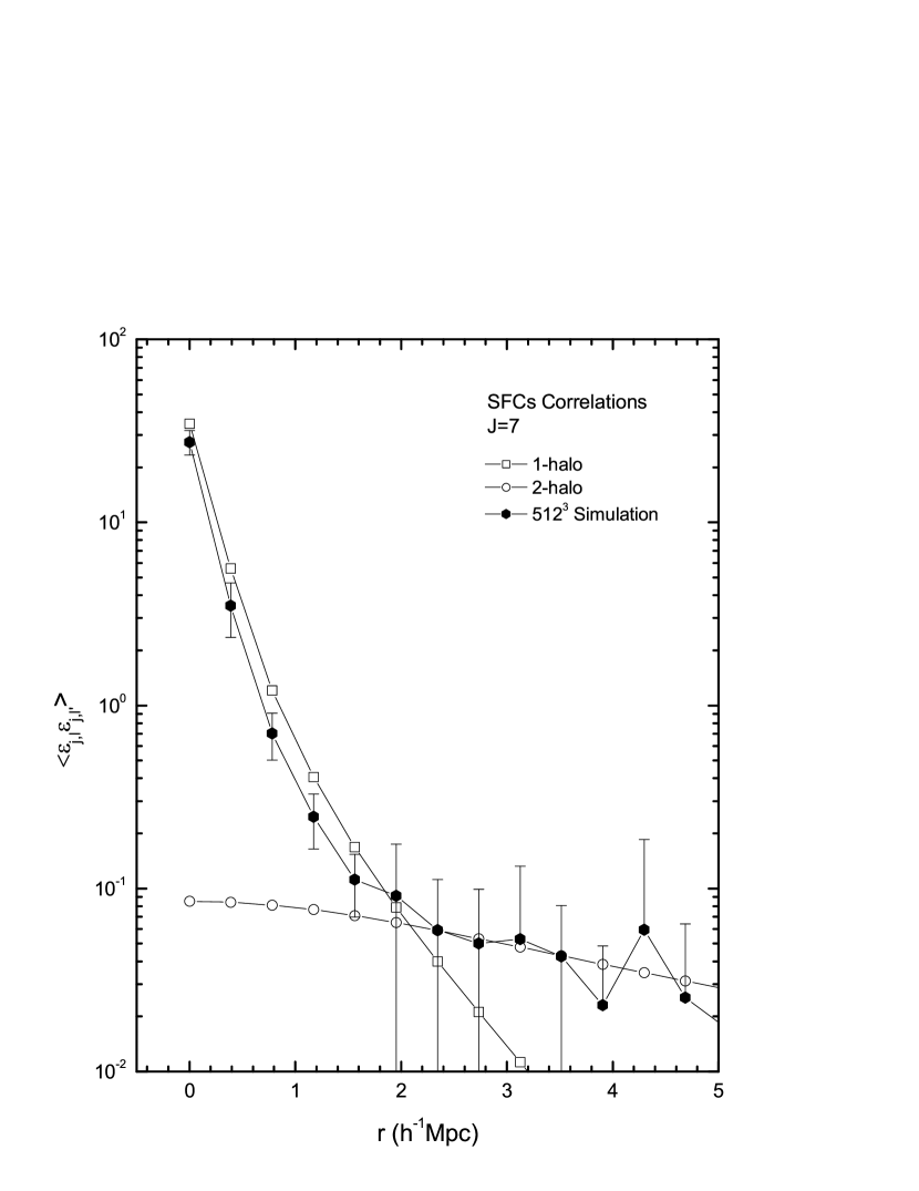
Figure 1: The SFC correlation function $\langle\epsilon_{\bf j,l}\epsilon_{\bf j,l^{\prime}}\rangle$ vs. $r$ for the simulation data (hexagon), 1-halo (square) and 2-halo (circle) terms. The scale ${\bf j}$ is taken to be $(7,7,7)$. The physical distance is given by $r=|{\bf l-l^{\prime}}|50/2^{j}$ h^-1 Mpc.

Figure 1 presents the $r$-dependence of $\langle\epsilon_{\bf j,l}\epsilon_{\bf j,l^{\prime}}\rangle$ at ${\bf j}=(7,7,7)$, corresponding to the smoothed field filtered on the linear scale $50/2^{7}=0.39$ h^-1 Mpc. The spatial distance between the cells ${\bf l}$ and ${\bf l^{\prime}}$ is $r=|{\bf l-l^{\prime}}|50/2^{7}$ h^-1 Mpc. In this calculation, we applied wavelet Daubechies 4 (Daubechies, 1992). As expected, the $r$- or $|{\bf l-l^{\prime}}|$-dependence of the correlation function $\langle\epsilon_{\bf j,l}\epsilon_{\bf j,l^{\prime}}\rangle$ shows the standard power law, $\langle\epsilon_{\bf j,l}\epsilon_{\bf j,l^{\prime}}\rangle\propto r^{-\alpha}$ with the index $\alpha\simeq 2$. That is, this correlation function is not localized. Meanwhile in Fig.1, the contributions of the 1-halo and 2-halo terms are also plotted, respectively. The 1-halo term is calculated from eq.(21) with the NFW density profiles of halos, and the 2-halo term is given by eq.(22) in which the correlation function $\xi({\bf r})$ is given by the linear power spectrum. The nonlinear clustering is largely due to the 1-halo term. Therefore, one can see that the nonlinear evolution of gravitational clustering cause correlations on scales of several Mpc.

4.3 Justifying the Quasi-Locality

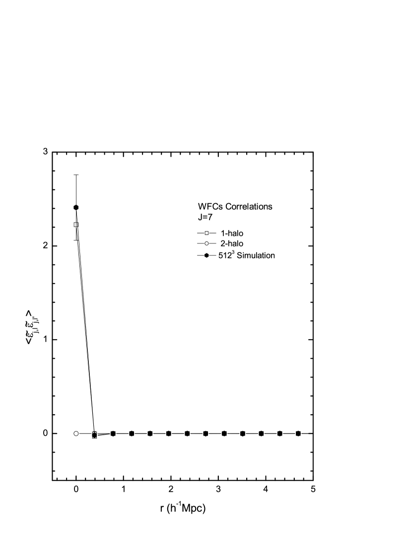
Figure 2: The DWT variable (WFC) correlation function $\langle\tilde{\epsilon}_{\bf j,l}\tilde{\epsilon}_{\bf j,l^{\prime}}\rangle$ vs. $r$ for the simulation data (hexagon), 1-halo (square) and 2-halo (circle) terms. The scale ${\bf j}$ is taken to be $(7,7,7)$. The physical distance is given by $r=|{\bf l-l^{\prime}}|50/2^{j}$ h^-1 Mpc.

We now study the quasi-locality of the clustering with the correlation function $\langle\tilde{\epsilon}_{\bf j,l}\tilde{\epsilon}_{\bf j^{\prime},l^{\prime}}\rangle$, which is used in the criterion $\kappa_{\bf j,j^{\prime}}(\Delta{\bf l})$ [eq.(13)]. First, we take the same parameter as Fig. 1, ${\bf j=j^{\prime}}=(7,7,7)$, and $r=|\Delta{\bf l}|50/2^{j}=|{\bf l-l^{\prime}}|50/2^{j}$ h^-1 Mpc, and also we used wavelet Daubechies 4 (Daubechies, 1992), which has $M=2$. The result of DWT correlation function $\langle\tilde{\epsilon}_{\bf j,l}\tilde{\epsilon}_{\bf j,l^{\prime}}\rangle$. is shown in Fig. 2. The solid circle at $r=0$ in Fig. 2 corresponds to $\Delta{\bf l}=0$, or ${\bf l=l^{\prime}}$, and other solid circles from left to right correspond, successively, to $\Delta{\bf l}=1$, 2, 3…

From Fig. 2, we can see immediately that the shape of the $r$- or $|\Delta{\bf l}|$-dependence of $\langle\tilde{\epsilon}_{\bf j,l}\tilde{\epsilon}_{\bf j,l^{\prime}}\rangle$ is quite different from the “standard” power law. The correlation function $\langle\tilde{\epsilon}_{\bf j,l}\tilde{\epsilon}_{\bf j,l^{\prime}}\rangle$ is non-zero mainly at point $r=0$ or $|\Delta{\bf l}|=0$. At $|\Delta{\bf l}|=1$, the correlation function $\langle\tilde{\epsilon}_{\bf j,l}\tilde{\epsilon}_{\bf j,l\pm 1}\rangle$ drops to tiny values around $\sim 0$. For $|\Delta{\bf l}|>1$, the correlation function basically is zero. The correlation length in terms of the position index ${\bf l}$ is approximately zero, namely, the covariance $\langle\tilde{\epsilon}_{\bf j,l}\tilde{\epsilon}_{\bf j,l^{\prime}}\rangle$ is diagonal. This is the spatial quasi-locality. In Fig. 2, we also plot the 1- and 2-halo terms, $\langle\tilde{\epsilon}_{\bf j,l}\tilde{\epsilon}_{\bf j,l^{\prime}}\rangle^{h}$ and $\langle\tilde{\epsilon}_{\bf j,l}\tilde{\epsilon}_{\bf j,l^{\prime}}\rangle^{hh}$. Although 1-halo term is dominated by massive halos, the covariance $\langle\tilde{\epsilon}_{\bf j,l}\tilde{\epsilon}_{\bf j,l^{\prime}}\rangle^{h}$ is also perfectly quasi-localized because of the self-similarity of density profiles of massive halos. The 2-halo term is zero at $r=0$, because, by definition, eq.(22) does not contain the contribution of autocorrelations of halos.

Figure 3 presents $\kappa_{\bf j,j^{\prime}}(\Delta{\bf l})$ vs. $r$, for ${\bf j}={\bf j^{\prime}}=(4,4,4)$, $(5,5,5)$ and $(6,6,6)$. The physical distance $r$ is the same as Fig. 2, given by $r=|\Delta{\bf l}|50/2^{j}=|{\bf l-l^{\prime}}|50/2^{j}$ h^-1 Mpc. The solid circle at $r=0$ corresponds to $|\Delta{\bf l}|=0$, at which, by definition, we have the normalization $\kappa_{\bf j,j}(0)=1$. Other points from small to large values of $r$ correspond to $\Delta{\bf l}=$ 1,2,…. successively. Clearly, all $\kappa_{\bf j,j}(\Delta{\bf l})$ for $\Delta l>0$ are less than $10^{-6}$, which is actually from the noises of sample. The result implies that for all calculable points of $r\geq 0$, the correlation is negligible, and satisfies the criterion eq.(13).

We also calculated $\kappa_{\bf j,j^{\prime}}(\Delta{\bf l})$ for modes of ${\bf j=j^{\prime}}=(j_{1},j_{2},j_{3})$, but $j_{1}\neq j_{2}\neq j_{3}$. Most of these cases shows $\kappa_{\bf j,j^{\prime}}(\Delta{\bf l})\simeq 0$ if $|\Delta{\bf l}|>0$. Only exception is for the cases of $j_{1},j_{2}<j_{3}$, and $|\Delta{\bf l}|=|l_{3}-l^{\prime}_{3}|=1$. As an example, Fig. 4 presents $\kappa_{\bf j,j}(\Delta{\bf l})$ for modes ${\bf j}=(5,5,6)$, and $r=|{\bf l_{3}-l^{\prime}_{3}}|50/2^{j_{3}}$. It shows that $\langle\tilde{\epsilon}_{\bf j,l}\tilde{\epsilon}_{\bf j,l^{\prime}}\rangle=0$ if $|l_{3}-l^{\prime}_{3}|>1$. The non-zero value at $|l_{3}-l^{\prime}_{3}|=1$ is about 20% of that at $\Delta l=0$. This result is consistent with the theorem (23), which only requires the suppression for modes $|l-l^{\prime}|>1$, but may not work for $|l-l^{\prime}|=1$. It implies that the clustering may give rise to the correlations between nearest neighbor cells in phase space. However, the cell resolved by $j_{1},j_{2}<j_{3}$ is a rectangle in the physical space, and the shortest edge is given by $j_{3}$, the physics distance of $|l_{3}-l^{\prime}_{3}|=1$ is still less than whole size of the rectangle. Thus, it could be concluded that the covariance $\langle\tilde{\epsilon}_{\bf j,l}\tilde{\epsilon}_{\bf j,l^{\prime}}\rangle$ is always quasi-diagonal in the sense that all members with ${\bf l}$ and ${\bf l^{\prime}}$ are almost zero if the distance $r$ between ${\bf l}$ and ${\bf l^{\prime}}$ is larger than the size of the cell $(j_{1},j_{2},j_{3})$ considered. In Fig. 4, we show also a result calculated with wavelets Daubechies 6 (D6), for which $M=3$. It yields about the same results as D4.

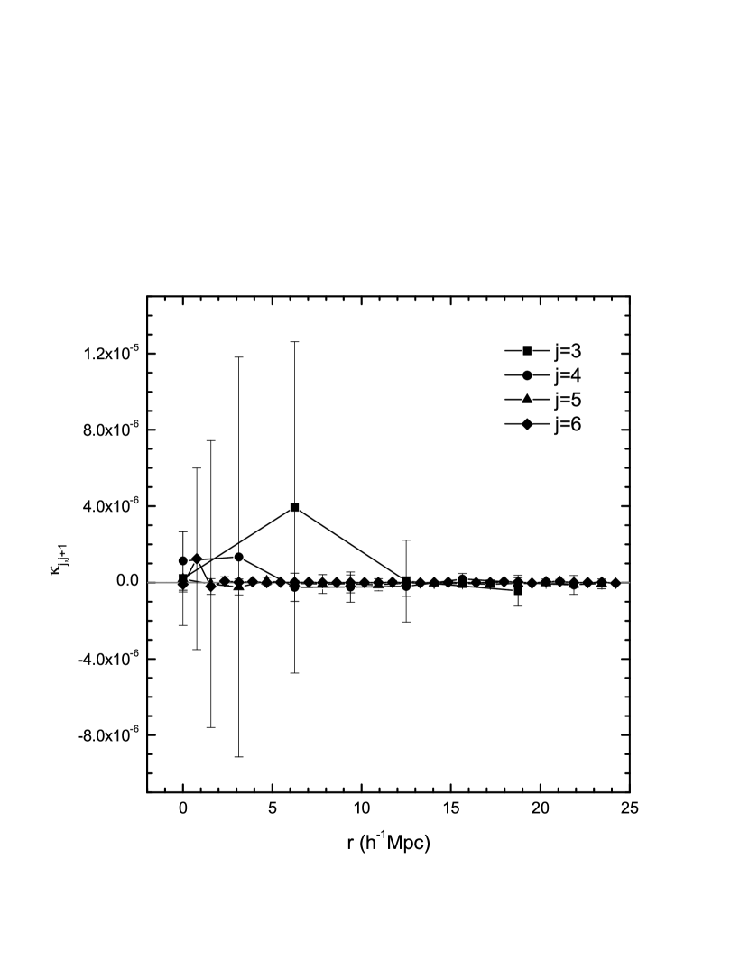
Figure 5: $\kappa_{\bf j,j+1}(\Delta{\bf l})$ vs. $r$ for the simulation data. The scale indexes are taken to be ${\bf j}=(j,j,j,)$, ${\bf j^{\prime}}=(j+1,j+1,j+1)$, and $j=3$, 4, 5 and 6, where $\Delta{\bf l}={\bf l}-{\bf l^{\prime}}/2$. The physical distance $r=|\Delta{\bf l}|50/2^{j}$ h^-1 Mpc.

For the correlation between modes $({\bf j,l})$ and $({\bf j^{\prime},l^{\prime}})$ with ${\bf j\neq j^{\prime}}$, we use the criterion $\kappa_{\bf j,j^{\prime}}$ of eq.(14). In this case, the physical distance between two cells is $r=|{\bf r}|$ and $r_{i}=|l_{i}/2^{j_{i}}-l^{\prime}_{i}/2^{j^{\prime}_{i}}|L$ h^-1 Mpc. Figure 5 plots $\kappa_{\bf j,j^{\prime}}(\Delta{\bf l})$ vs. $r$ for modes ${\bf j}=(j,j,j)$, ${\bf j^{\prime}}=(j+1,j+1,j+1)$, and $j=3,4,5$ and 6. All the values of $\kappa_{\bf j,j^{\prime}}(\Delta{\bf l})$ in Fig. 5 are not larger than $10^{-5}$, and are much less than the diagonal terms $\langle\tilde{\epsilon}^{2}_{\bf j,l}\rangle$, or $\langle\tilde{\epsilon}^{2}_{\bf j,l^{\prime}}\rangle$. We found this result is generally true for all the cases of ${\bf j\neq j^{\prime}}$. That is, the second order correlation between two modes with different scales ${\bf j}$ and ${\bf j^{\prime}}$ are always negligible, regardless the indices ${\bf l}$ and ${\bf l^{\prime}}$. In other words, the covariance of the WFC variables $\langle\tilde{\epsilon}_{\bf j,l}\tilde{\epsilon}_{\bf j^{\prime},l^{\prime}}\rangle$ generally are quasi-diagonal.

As for the high order statistics by criterion eqs.(15) and (16), we can cite some previous calculations of the non-local scale-scale correlation defined by

$$C^{2,2}_{\bf j,j}(\Delta{\bf l})=\frac{\langle\tilde{\epsilon}^{2}_{\bf j,l}\tilde{\epsilon}^{2}_{\bf j,l+\Delta l}\rangle}{\langle\tilde{\epsilon}^{2}_{\bf j,l}\rangle\langle\tilde{\epsilon}^{2}_{\bf j,l+\Delta l}\rangle}.$$ (28)

which is the criterion eq.(15) with $p=q=2$. It has been shown that either for the APM bright galaxy catalog (Loveday et al. 1992) or mock samples of galaxy survey (Cole et al. 1998), the non-local scale-scale correlation always yields $|C^{2,2}_{\bf j,j}(\Delta{\bf l})-1|\ll 1$ if $\Delta{\bf l}>0$ (Feng, Deng & Fang 2000). Although this work was not for addressing the problem of the quasi-locality, the result did support the quasi-locality up to the 4^th order statistics.

4.4 Non-Gaussianity Revealed by DWT Variables

As discussed in §2.3, it is necessary to show that the random variables $\tilde{\epsilon}_{\bf j,l}$ are non-Gaussian for evolved fields. The possible non-Gaussian features with the DWT variables are (1) non-Gaussian one-point distribution of $\tilde{\epsilon}_{\bf j,l}$, and (2) local scale-scale correlations (§3.3).

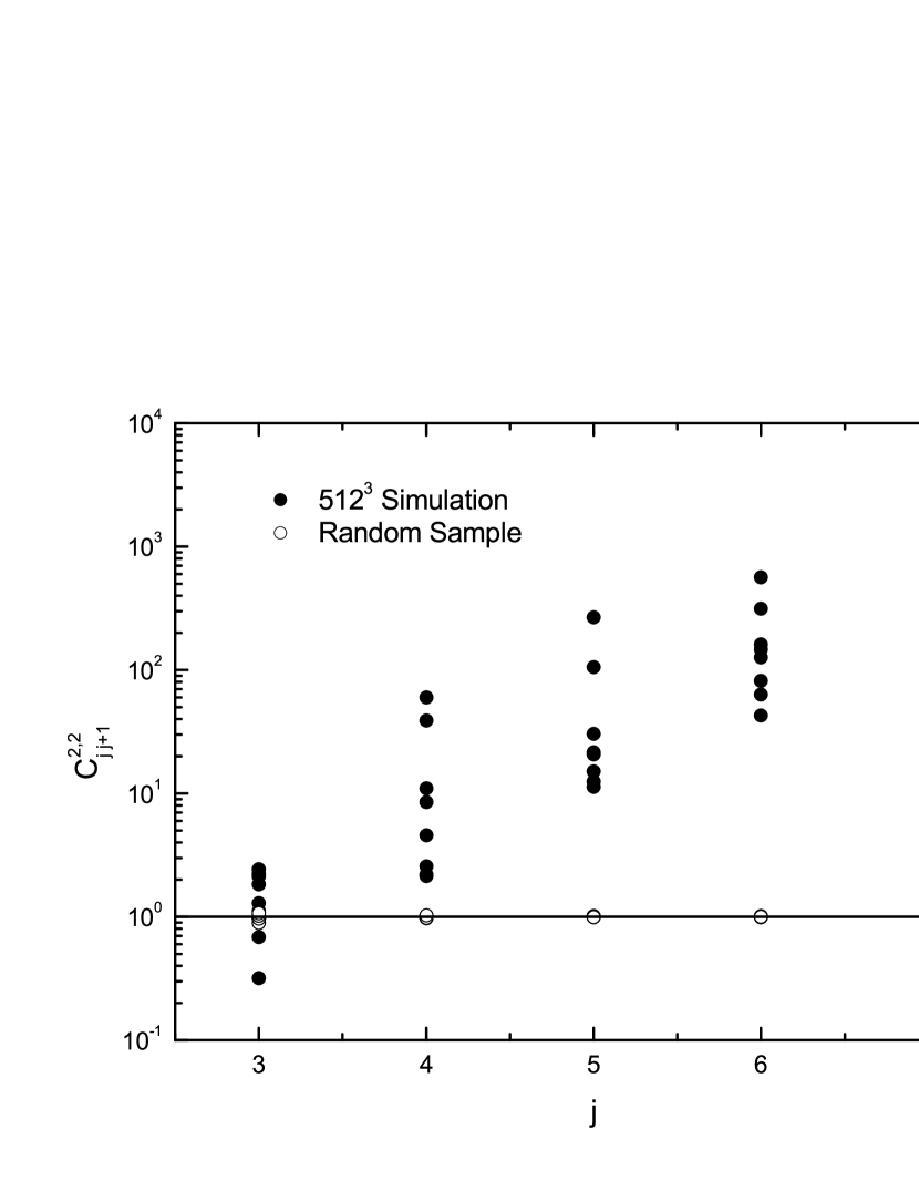
Figure 7: The 4^th local scale-scale correlation $C^{2,2}_{\bf j,j+1}(\Delta{\bf l}=0)$ vs. $j$ for the simulation data (solid circle) and Gaussian random sample (circle).

In Fig. 6, we plot the one-point distribution on scales ${\bf j}=(j,j,j,)$ and $j=$ 5, 6, 7 and 8. It illustrates that the kurtosis of the one-point distribution is high. The PDF (probability distribution function) is approximately lognormal. The 4^th order local scale-scale correlation $C^{2,2}_{\bf j,j}(\Delta{\bf l}=0)$ is plotted in Fig. 7. It shows $C^{2,2}_{\bf j,j}(\Delta{\bf l}=0)\gg 1$ on small scales ($j=$ 5,  6 and 7), while random data gives $C^{2,2}_{\bf j,j}(\Delta{\bf l}=0)=1$ on all scales. The evolved field is highly non-Gaussian, although it is always quasi-localized.

5 Discussions and Conclusions

We showed that the cosmic clustering behavior is quasi-localized. If the field is viewed by the DWT modes in phase space, the nonlinear evolution will give rise to the coupling between modes on different scales but in the same physical area, and the coupling between modes at different position is weak. The quasi-local evolution means that, if the initial perturbations in a waveband $k\pm\Delta k/2$ and at different space range $\Delta x$ is uncorrelated, the evolved perturbations in this waveband at different space range $\Delta x$ will also be uncorrelated, or very weakly correlated. In this sense, the nonlinear evolution has memory of its initial spatial correlation in the phase space. This memory is essentially from the hierarchical and self-similar feature of the mass field evolution. The density profiles of massive halos obey the scaling law [eq.(18)], and therefore, the contributions to the non-local correlation function from various halos are uniformly suppressed.

It has been realized about ten years ago that some random fields generated by a self-similar hierarchical process generally shows locality of their auto-correlation function in the phase space, if the initial field is local, like a Gaussian field (Ramanathan & Zeitouni, 1991; Tewfik & Kim 1992; Flandrin, 1992). Later, this result are found to be correct for various models of structure formations via hierarchical cascade stochastic processes (Greiner et al. 1996, Greiner, Eggers & Lipa, 1998). These studies implies that the local evolution and initial perturbation memory seems to be generic of self-similar hierarchical fields, regardless the details of the hierarchical process. It has been pointed out that models for realizing the self-similar hierarchical evolution of cosmic mass field, such as the fractal hierarchy clustering model (Soneira & Peebles 1977), the block model (Cole & Kaiser 1988), merging cell (Rodrigues & Thomas 1996), have the same mathematical structures as hierarchical cascade stochastic models applied in other fields (Pando et al 1998, Feng, Pando & Fang 2001). Obviously, the local evolution can be straightforward obtained in those models.

The DWT analysis is effective to reveal the quasi-locality in phase space. Such quasi-locality is hardly described by the Fourier modes $\hat{\delta}({\bf k})$, as the information of spatial positions is stored in the phases of all Fourier modes. Moreover, the Fourier amplitudes $|\hat{\delta}({\bf k})|$ subject to the central limit theorem, and are insensitive to non-Gaussianity. The wavelet basis, however does not subject to the central limit theorem (Pando & Fang 1998), which enable us to measure all the quasi-local features with the statistics of $\tilde{\epsilon}_{\bf j,l}$.

The quasi-locality of the DWT correlation is essential for recovery of the primordial power spectrum using a localized mapping in phase space. Such mapping has been developed in recovering the initial Gaussian power spectrum from evolved field in the quasi-linear regime (Feng & Fang 2000). By virtue of the quasi-locality in fully developed fields, we would be able to generalize the method of localized mapping in phase space to highly non-linear regime.

The quasi-local evolution may also provide the dynamical base for the lognormal model (Bi, 1993; Bi & Davidsen 1997, Jones 1999). The basic assumption of the lognormal model is that the non-linear field can be approximately found from the corresponding linear Gaussian field by a local exponential mapping. The local mapping is supported by the quasi-local evolution. We see from Fig. 6 that the PDF of evolved field is about lognormal. Therefore, in the context of quasi-local evolution, a local (exponential) mapping from the linear Gaussian field to a lognormal field might be a reasonable sketch of the nonlinear evolution of the cosmic density field.

Figure 3: $\kappa_{\bf j,j}$ vs. $r$ for the simulation data. ${\bf j}$ are taken to be $(4,4,4)$ (top panel), (5,5,5) (middle), and (6,6,6) (bottom). The physical distance is given by $r=|{\bf l-l^{\prime}}|50/2^{j}$ h^-1 Mpc.

Figure 4: $\kappa_{\bf j,j^{\prime}}(\Delta l)$ vs. $r$ for the simulation data. The scales are ${\bf j}=(5,5,6)$ The physical distance $r=|\Delta{\bf l}|50/2^{6}$ h^-1 Mpc. Wavelets D4($M=2$) and D6($M=3$) are used.

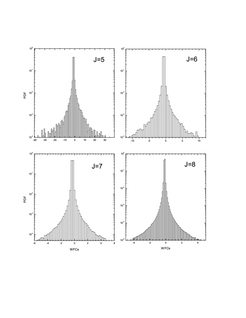
Figure 6: The one-point distribution of $\tilde{\epsilon}_{\bf j,l}$ for ${\bf j}=(j,j,j,)$ and $j=$ 5, 6, 7 and 8.

References

• (1)
• (2) Bardeen, J., Bond, J., Kaiser, N. & Szalay, A. 1986, ApJ, 304, 15
• (3)
• (4) Bi, H.G. 1993, ApJ, 405, 479
• (5)
• (6) Bi, H.G & Davidsen, A. F. 1997, ApJ, 479, 523.
• (7)
• (8) Cole S. and Kaiser, N. 1988, MNRAS, 233, 637
• (9)
• (10) Cooray, A. and Sheth, R. 2002, Physics Reports, 372, 1latex
• (11)
• (12) Croft, R.A.C., Weinberg, D., Katz, N. & Hernquist, L. 1998, ApJ, 495, 44
• (13)
• (14) Daubechies I. 1992, Ten Lectures on Wavelets (Philadelphia: SIAM)
• (15)
• (16) Fang, L.Z. & Feng, L.L. 2000, ApJ, 539, 5
• (17)
• (18) Fang, L.Z. and Thews, R. 1998, Wavelets in Physics, World Scientific, (Singapore)
• (19)
• (20) Feng, L.L., Deng, Z.G. & Fang, L.Z. 2000, ApJ, 530, 53
• (21)
• (22) Feng, L.L. & Fang, L.Z. 2000, ApJ, 535, 519
• (23)
• (24) Flandrin, P., 1992, IEEE Trans. Inf. Theory, 1992, 38, 910
• (25)
• (26) Greiner, M., Eggers, H.C. & Lipa, P. 1998, Phys. Rev. Lett. 80, 5333
• (27)
• (28) Greiner, M., Giesemann, J., Lipa, P., and Carruthers, P. 1996, Z. Phys. C69, 305
• (29)
• (30) Greiner, M., Lip, P., & Carruthers, P., 1995, Phys. Rev. E51, 1948.
• (31)
• (32) Jing, Y.P., & Suto, Y., 2002, ApJ, 574, 538
• (33)
• (34) Jones, B.T., 1999, MNRAS, 307, 376
• (35)
• (36) Meneveau, C. & Sreenivasan, K.R. 1987, Phys. Rev. Lett. 59, 1424
• (37)
• (38) Monaco, P. & Efstathiou, G. 2000, MNRAS,308,763
• (39)
• (40) Moore, B., Governato, F., Quinn, T., Stadel, J. & Lake, G., 1999, MNRAS, 261, 827
• (41)
• (42) Narayanan, V. & Weinberg, D. 1998, ApJ, 508, 440
• (43)
• (44) Navarro, J., Frenk, C. & White, S. 1996, ApJ, 462, 563
• (45)
• (46) Neyman, J. & Scott, E.L. 1952, ApJ, 116, 144
• (47)
• (48) Pando, J. & Fang, L.Z. 1998, A&A, 340, 335
• (49)
• (50) Pando, J. Feng, L.L. & Fang, L.Z. 2001, ApJ, 554, 841
• (51)
• (52) Pando, J., Lipa, P., Greiner, M. and Fang, L.Z. 1998, ApJ, 496, 9
• (53)
• (54) Press, W.H. & Schechter, P. 1974, ApJ, 187, 425
• (55)
• (56) Peebles, P. 1980, The large scale structures of the universe, (Princeton press)
• (57)
• (58) Ramanathan, J. & Zeitouni, O. 1991, IEEE Trans. Inf. Theory, 37, 1156
• (59)
• (60) Rodrigues, D.D.C. & Thomas, P.A. 1996, MNRAS282, 631
• (61)
• (62) Scherrer, R.J. & Bertschinger, E. 1991, ApJ, 381, 349
• (63)
• (64) Soneira, R.M. & Peebles, P.J.E. 1977, ApJ, 211, 1
• (65)
• (66) Spergel, D.N. et al 2003, astro-ph/0302209
• (67)
• (68) Tewfik, A.H. and Kim, M. 1992, IEEE Trans. Inf. Theory, 38, 904
• (69)
• (70) Zel’dovich, Ya.B. 1970, A & A, 5, 84
• (71)
Refer to caption