THE ELECTROMAGNETIC SIGNATURE OF BLACK HOLE RINGDOWN

abstract

We investigate generation of electromagnetic radiation by gravitational waves interacting with a strong magnetic field in the vicinity of a vibrating Schwarzschild black hole. Such an effect may play an important role in gamma-ray bursts and supernovae, their afterglows in particular. It may also provide an electromagnetic counterpart to gravity waves in many situations of interest, enabling easier extraction and verification of gravity wave waveforms from gravity wave detection. We set up the Einstein-Maxwell equations for the case of odd parity gravity waves impinging on a static magnetic field as a covariant and gauge-invariant system of differential equations which can be integrated as an initial value problem, or analysed in the frequency domain. We numerically investigate both of these cases. We find that the black hole ringdown process can produce substantial amounts of electromagnetic radiation from a dipolar magnetic field in the vicinity of the photon sphere.

1 Introduction

In recent years there has been an enormous effort worldwide to detect gravitational radiation (see, e.g., Barich and Weiss (1999); Willke et al. (2002); Ando et al. (2002); Acernese et al. (2002)). It is hoped that within the next few years these detectors will be able to consistently detect and measure the gravity waves (GW) emitted from such events as black hole (BH) merger (Buonanno, 2002) and exploding and collapsing stars. A pressing problem for these detectors is the extraction of the actual waveform from the huge amount of noise invariably generated in the detection process. The race is currently on to calculate these waveforms in every conceivable situation in order that gravity wave signatures can eventually be statistically extracted from the noise continuously generated by these detectors (Flanagan and Hughes, 1998a, b; Nicholson and Vecchio, 1998), a formidable task. We discuss here a mechanism describing how many of these events could be accompanied by an electromagnetic (EM) counterpart with the same waveform, which could considerably aid in this process.

Many events will be accompanied by an optical counterpart, such as in supernovae (SN) II and some compact binary mergers (Sylvestre, 2003), but many in general will not, such as BH-BH merger, and BH ringdown. In any case these will only tell us to expect detection, and not the precise form of the waveform to try to extract. What would be highly useful for GW detection would be a simultaneous optical detection of the event with the EM waveform mirroring that of the GW. This is the situation we discuss here.

When a plane gravity wave passes through a magnetic field, it vibrates the magnetic field lines, thus creating EM radiation with the same frequency as the forcing GW, an effect which has been known for some time (see, e.g.,  Cooperstock (1968); Gerlach (1974); Marklund, Brodin, and Dunsby (2000) and references therein). This would provide exactly the mechanism required: virtually all stars have a strong magnetic field threading through and surrounding them, and this field becomes immensely strong as the field lines are compressed as the star collapses to a BH or neutron star; anything up to $10^{14}$G – possibly even higher – seems possible in magnetars (Kouveliotou et al., 1998).

It has been proposed that this mechanism may indeed have been observed, being partly responsible for the afterglow observed in some gamma-ray bursts (GRB) and SN events, an argument strengthened by certain anomalous GRB and SN light curves (see Mosquera Cuesta (2002) and references therein for a detailed discussion). The basic idea is that these events are thought to form a BH or neutron star after the initial explosion (envelope ejection), surrounded by a thin plasma which can support a strong magnetic field able to reach supercritical values over a relatively long period of time (compared to the period of the emitted GW). The formation of the compact object will release a substantial fraction of its mass as GW which could then be converted into EM radiation as it passes through the plasma. Individual models differ considerably in many respects; in particular, additional GW may be produced from a stressed accretion disk powered by the spin of the BH (van Putten, 2001).

Studies of generation of EM radiation by GW in astrophysical situations so far have provided order of magnitude estimates (Mosquera Cuesta, 2002) and some of the extra complexities involved when a thin plasma is present (Macedo and Nelson, 1983; Daniel and Tajima, 1997; Brodin and Marklund, 1999; Marklund, Brodin, and Dunsby, 2000; Servin, Brodin, and Marklund, 2001). In particular, a thin plasma can increase the frequency of the electromagnetic radiation, whose origin is from a plane gravity wave passing through a uniform, static, magnetic field, thus strengthening the observational potential of the EM-GW interaction still further (Brodin, Marklund, and Servin, 2001; Servin and Brodin, 2003). While these investigations have given a good indication of the physical processes we may expect, the effect has not yet been studied in a strong gravitational field, the most promising place we may expect such an interaction as likely to happen.

Our aim here, then, is to study the induced EM field from the interaction of GW emitted during BH ringdown, the settling down of a BH after an initial perturbation, with a strong magnetic field which surrounds the BH. Shortly after a BH is disturbed by any kind of small perturbation, it radiates its curvature deformations as GW with certain characteristic frequencies which are independent of the initial perturbation, and dependent only on its mass (in the case of a Schwarzschild BH, which we consider here). These complex quasi-normal frequencies form solutions known as quasi-normal modes which govern the BH ringdown process (Nollert, 1999; Kokkotas and Schmidt, 1999). As the ringdown process is thought to be independent of the initial perturbation, we may expect that studying this particular situation will help give understanding in more complex situations, such as the late stages of BH-BH merger (Buonanno, 2002). Indeed, while it would seem logical that perturbations of Schwarzschild would give little information about something as non-linear as colliding black holes, it turns out that perturbation theory gives surprising accuracy in many cases of interest (Price and Pullin, 1994).

The frequency of this generated EM radiation will be very low, generally less than about $100$kHz, and would be typically absorbed by the interstellar medium. This is where the photon frequency conversion (Marklund, Brodin, and Dunsby, 2000; Brodin, Marklund, and Servin, 2001; Servin and Brodin, 2003) could come into play, overcoming this by increasing the frequency to detectable levels. An important extension of this work, therefore, will be to include a plasma into this situation; we leave this to later, and concentrate here on setting up a suitable formalism for the inclusion of a plasma, while investigating the pure curvature effects of the BH, which turn out to be quite large. We find that the amplification of the EM field is much stronger than is the case of plane GW (Marklund, Brodin, and Dunsby, 2000), where the amplification grows linearly with interaction distance. Here, we find substantial growth in the vicinity of the horizon and photon sphere.

1.1 An overview

Electromagnetic waves around a Schwarzschild BH generated by gravitational waves interacting with a strong static magnetic field are governed by the Einstein-Maxwell equations which are of the form

$$\mbox{EM field around a BH}=\left(\mbox{{GW}}\times\mbox{{Strong static magnetic field}}\right).$$ (1-1)

The homogeneous solution to these equations, where the induced currents are zero, will be governed by the well known Regge-Wheeler (RW) equation for EM perturbations around a BH (Price, 1972), while the GW terms are governed by the Regge-Wheeler equation for gravitational perturbations of a BH (Regge and Wheeler, 1957). The RW equation describes how the fields of different spin are lensed and scattered around the hole. A description of the more general situation including the rhs of Eq. (1-1) is rather less trivial than Eq. (1-1) may suggest, for several reasons: for example, the GW terms on the rhs need some manipulation to convert them to the familiar RW variable, and the existence of the magnetic field on both sides of the equation means that gauge problems are paramount, and considerable work must be done to cast the equations into a manifestly gauge-invariant form. While it may be expedient to use the Newman-Penrose formalism (Chandrasekhar, 1983) for this problem as all variables in the perturbed spacetime travel on null cones, an important extension of this work will be to include plasma effects, to model a more realistic astrophysical environment, for which the Newman-Penrose formalism is not so adept. In addition, the electric and magnetic fields require a timelike vector field for their definition. For these reasons we will use the covariant and gauge-invariant perturbation method introduced in Clarkson and Barrett (2003), which is ideally suited to this particular problem involving spherical symmetry, and has the advantage that is is well adapted to fluids for later use when investigating plasma effects.

An important issue in relativistic perturbation theory is the mapping, or gauge choice, one makes between the background and perturbed model; many perturbation approaches are not invariant with respect to this gauge choice. Metric based approaches to perturbation theory suffer from this gauge freedom, whereby spurious gauge modes exist and must be identified. While these spurious gauge modes may be eliminated in analytical treatments, when the equations are integrated numerically these modes have a tendency to grow very fast without bound, in so-called gauge pathologies (Alcubierre, 1998). Furthermore, the tractability of the problem often depends upon judicious gauge choice; hardly an ideal situation (Ruoff, Stavridis, and Kokkotas, 2001).

The covariant ‘1+1+2’ approach we utilise relies on the introduction of a partial frame which form the differential operators of the spacetime, and allow all objects to be split into invariantly defined physical or geometric objects. Covariant perturbation techniques initiated in Ellis and Bruni (1989) are employed to write the equations in a fully gauge-invariant form which can then be solved with the use of appropriate harmonic functions which remove the tensorial nature of the equations. To aid in the solution we consider it formally as a second-order perturbation problem, and introduce ‘interaction variables’ for quadratic quantities. This then allows us to write the equations for the induced EM radiation as a system of gauge-invariant, covariant, first order ordinary differential equations in the relevant variables, while we can easily convert to covariant wave equations for clarity and integration as an initial value problem when desired.

The paper is organised as follows. The covariant formalism we use is reviewed in Sec. 2. In Sec 3 we derive the coupled perturbation equations which govern the interaction. These equations are integrated numerically in Sec. 4, and the implications for the emitted radiation discussed. We briefly conclude in Sec. 5. An Appendix gives some key formulae relating to the spherical harmonics we use.

Sections 2 and 3 contain most of the technical material, the crucial results being Eqs. (3-41) – (3-43) and (3-45); some readers may wish to skip to Section 4 where specific astrophysical situations are discussed.

2 The 1+1+2 covariant approach

Covariant methods in General Relativity (GR) are formulated in a very different way from coordinate metric based approaches: in the latter, Einstein’s field equations (EFE) are second order partial differential equations in the components of the metric; in the former, a physical (partial) frame is chosen and the Ricci and Bianchi identities are irreducibly split with respect to this frame, resulting in a system of first-order differential equations. Supplemented by the crucial commutation relations between the frame vectors, this system of equations becomes equivalent to the EFE, but always deals with invariantly defined physical or geometric quantities.

The 1+1+2 covariant sheet approach relies on the introduction of two frame vectors: the first being a timelike vector field $u^{a}$: $u^{a}u_{a}=-1$, representing the congruence on which observers sit; the second is a spacelike vector field $n^{a}$: $n^{a}n_{a}=1,~{}n^{a}u_{a}=0$, which can be chosen along a preferred direction of the spacetime. These two vector fields define a projection tensor

$$N_{a}^{~{}b}\equiv h_{a}^{~{}b}-n_{a}n^{b}=g_{a}^{~{}b}+u_{a}u^{b}-n_{a}n^{b},$$ (2-1)

which projects vectors orthogonal to $n^{a}$ and $u^{a}$: $n^{a}N_{ab}=0=u^{a}N_{ab}$, onto 2-surfaces ($N_{a}^{~{}a}=2$) which we refer to as the ‘sheet’; $h_{ab}=g_{ab}+u_{a}u_{b}$ is the tensor which projects orthogonal to $u^{a}$, into the observers’ rest space. Using $h_{ab}$, any 4-vector may be split into a (1+3 scalar) part parallel to $u^{a}$ and a (1+3-vector) part orthogonal to $u^{a}$. Any second rank tensor may be covariantly and irreducibly split into scalar, 3-vector and projected, symmetric, trace-free (PSTF) 3-tensor parts, which requires the alternating tensor $\varepsilon_{abc}=u^{d}\eta_{dabc}$; these are the key quantities in the 1+3 covariant approach (Ellis and van Elst, 1998). Crucially, the covariant derivative of $u^{a}$ may be split in the standard manner, the irreducible parts (the acceleration $\dot{u}^{a}$, the expansion, $\theta$, the shear, $\sigma_{ab}$, and the rotation, $\omega^{a}$) forming some of the key variables of the 1+3 approach – we refer to Ellis and van Elst (1998) for further details.

Now, using $N_{ab}$, any 3-vector $\psi^{a}$ can now be irreducibly split into a scalar, $\Psi$, which is the part of the vector parallel to $n^{a}$, and a 2-vector, $\Psi^{a}$, lying in the sheet orthogonal to $n^{a}$:

$$\psi^{a}=\Psi n^{a}+\Psi^{a},$$ (2-2a)

where

$$\Psi\equiv\psi_{a}n^{a},~{}~{}~{}\mbox{and}~{}~{}~{}\Psi^{a}\equiv N^{ab}\psi_{b}\equiv\psi^{\bar{a}},$$ (2-2b)

where we use a bar over an index to denote projection with $N_{ab}$. Similarly, any PSTF tensor, $\psi_{ab}$, can now be split into scalar, vector and 2-tensor (which are PSTF with respect to $n^{a}$, and is therefore transverse-traceless) parts:

$$\psi_{ab}=\psi_{\langle ab\rangle}=\Psi\left(n_{a}n_{b}-\tfrac{1}{2}N_{ab}\right)+2\Psi_{(a}n_{b)}+\Psi_{{ab}},$$ (2-3a)

where

$$\Psi \equiv n^{a}n^{b}\psi_{ab}=-N^{ab}\psi_{ab},$$ (2-3b)

$$\Psi_{a} \equiv N_{a}^{~{}b}n^{c}\psi_{bc}=\Psi_{\bar{a}},$$ (2-3c)

$$\Psi_{ab} \equiv \psi_{\{ab\}}\equiv\left(N_{(a}^{~{}~{}c}N_{b)}^{~{}~{}d}-\tfrac{1}{2}N_{ab}N^{cd}\right)\psi_{cd}.$$ (2-3d)

We use curly brackets to denote the transverse-traceless (TT) part of a tensor. We also define the alternating Levi-Civita 2-tensor (area element)

$$\varepsilon_{ab}\equiv\varepsilon_{abc}n^{c}=u^{d}\eta_{dabc}n^{c},$$ (2-4)

so that $\varepsilon_{ab}n^{b}=0=\varepsilon_{(ab)}$.

With these definitions, then, we may split any object into scalars, 2-vectors in the sheet, and transverse-traceless 2-tensors, also defined in the sheet. These three types of objects are the only objects which need to be solved for, after a complete splitting. Hereafter, we will assume such a split has been made, and ‘vector’ will generally refer to a vector projected orthogonal to $u^{a}$ and $n^{a}$, and ‘tensor’ will generally mean transverse-traceless tensor, defined by Eq. (2-3).

We split the familiar 1+3 variables in this manner; in particular, the electric and magnetic fields are irreducibly split

$$E^{a} = \mathscr{E}n^{a}+\mathscr{E}^{a},$$ (2-5a)

$$B^{a} = \mathscr{B}n^{a}+\mathscr{B}^{a},$$ (2-5b)

while the kinematical and gravitational variables become, using Eqs. (2-2b) and (2-3)

$$\dot{u}^{a} = {\cal A}n^{a}+{\cal A}^{a},$$ (2-6a)

$$\omega^{a} = \Omega n^{a}+\Omega^{a},$$ (2-6b)

$$\sigma_{ab} = \Sigma\left(n_{a}n_{b}-\tfrac{1}{2}N_{ab}\right)+2\Sigma_{(a}n_{b)}+\Sigma_{ab},$$ (2-6c)

$$E_{ab} = {\cal E}\left(n_{a}n_{b}-\tfrac{1}{2}N_{ab}\right)+2{\cal E}_{(a}n_{b)}+{\cal E}_{ab},$$ (2-6d)

$$H_{ab} = {\cal H}\left(n_{a}n_{b}-\tfrac{1}{2}N_{ab}\right)+2{\cal H}_{(a}n_{b)}+{\cal H}_{ab}.$$ (2-6e)

For example, ${\cal E}=n^{a}n^{b}E_{ab}$ is the tidal force along $n^{a}$, ${\cal E}_{a}=N_{a}^{~{}b}n^{c}E_{bc}$ is a ’drift’ vector, while ${\cal E}_{ab}=E_{\{ab\}}$ is the TT part of the electric Weyl curvature in the sheet orthogonal to $n^{a}$.

There are two new derivatives of interest, which $n^{a}$ defines, for any object $\psi_{\cdots}^{~{}~{}\cdots}$:

$$\!\!\!\!\!\!\!\!\!\hat{\psi}_{a\cdots b}^{~{}~{}~{}~{}~{}c\cdots d} \equiv n^{e}{\mathrm{D}}_{e}\psi_{a\cdots b}^{~{}~{}~{}~{}~{}c\cdots d},$$ (2-7a)

$$\!\!\!\!\!\!\!\!\!\delta_{e}\psi_{a\cdots b}^{~{}~{}~{}~{}~{}c\cdots d} \equiv N_{e}^{~{}j}N_{a}^{~{}f}\cdots N_{b}^{~{}g}N_{h}^{~{}c}\cdots N_{i}^{~{}d}{\mathrm{D}}_{j}\psi_{f\cdots g}^{~{}~{}~{}~{}~{}h\cdots i},$$ (2-7b)

where $\mathrm{D}_{a}$ is the spatial derivative defined by $h_{a}^{~{}b}$ (see, e.g.,  Ellis and van Elst (1998)) . The hat-derivative is the derivative along the vector field $n^{a}$ in the surfaces orthogonal to $u^{a}$. It is important to note, however, that these derivatives do not commute; commutation relations for scalars are given in Clarkson and Barrett (2003). This is a vital aspect of the formalism.

With these definitions we may now decompose the spatial projection of the covariant derivative of $n^{a}$ orthogonal to $u^{a}$:

$${\mathrm{D}}_{a}n_{b}=n_{a}a_{b}+\tfrac{1}{2}\phi N_{ab}+\xi\varepsilon_{ab}+\zeta_{ab},$$ (2-8)

where

$$a_{a} \equiv n^{c}{\mathrm{D}}_{c}n_{a}=\hat{n}_{a},$$ (2-9a)

$$\phi \equiv \delta_{a}n^{a},$$ (2-9b)

$$\xi \equiv \tfrac{1}{2}\varepsilon^{ab}\delta_{a}n_{b},$$ (2-9c)

$$\zeta_{ab} \equiv \delta_{\{a}n_{b\}}.$$ (2-9d)

We may interpret these as follows: travelling along $n^{a}$, $\phi$ represents the sheet expansion, $\zeta_{ab}$ is the shear of $n^{a}$ (distortion of the sheet), and $a^{a}$ its acceleration, while $\xi$ represents a ‘twisting’ of the sheet – the rotation of $n^{a}$. The other derivative of $n^{a}$ is its change along $u^{a}$,

$$\dot{n}_{a}={\cal A}u_{a}+\alpha_{a}~{}~{}~{}\mbox{where}~{}~{}~{}\alpha_{a}\equiv\dot{n}_{\bar{a}}~{}~{}~{}\mbox{and}~{}~{}~{}{\cal A}=n^{a}\dot{u}_{a}.$$ (2-10)

The new variables $a_{a}$, $\phi$, $\xi$, $\zeta_{ab}$ and $\alpha_{a}$ are fundamental objects in the spacetime, and their dynamics gives us information about the spacetime geometry. They are treated on the same footing as the kinematical variables of $u^{a}$ in the 1+3 approach (which also appear here).

The 1+1+2 split of the Ricci identities for $u^{a}$ and $n^{a}$, and the Bianchi identities, provide a complete set of first-order differential equations for these variables, and were discussed in Clarkson and Barrett (2003) for the case of a gravitationally perturbed BH. We shall not require a further generalisation of these equations here.

Obviously, we shall require Maxwell’s equations (ME), which may be irreducibly split using these definitions:

$$\hat{\mathscr{E}}+\delta_{a}\mathscr{E}^{a} = -\phi\mathscr{E}+\mathscr{E}_{a}a^{a}+2\Omega\mathscr{B}+2\Omega^{a}\mathscr{B}_{a}+\mu_{0}\rho_{\mathrm{e}},$$ (2-11a)

$$\hat{\mathscr{B}}+\delta_{a}\mathscr{B}^{a} = -\phi\mathscr{B}+\mathscr{B}_{a}a^{a}-2\Omega\mathscr{E}-2\Omega^{a}\mathscr{E}_{a},$$ (2-11b)

$$\dot{\mathscr{E}}-\varepsilon_{ab}\delta^{a}\mathscr{B}^{b} = 2\xi\mathscr{B}+\mathscr{E}^{a}\alpha_{a}-\left(\tfrac{2}{3}\theta-\Sigma\right)\mathscr{E}+\Sigma^{a}\mathscr{E}_{a}+\varepsilon_{ab}\left({\cal A}^{a}\mathscr{B}^{b}+\Omega^{a}\mathscr{E}^{b}\right)-\mu_{0}{\cal J},$$ (2-11c)

$$\dot{\mathscr{B}}+\varepsilon_{ab}\delta^{a}\mathscr{E}^{b} = -2\xi\mathscr{E}+\mathscr{B}^{a}\alpha_{a}-\left(\tfrac{2}{3}\theta-\Sigma\right)\mathscr{B}+\Sigma^{a}\mathscr{B}_{a}-\varepsilon_{ab}\left({\cal A}^{a}\mathscr{E}^{b}-\Omega^{a}\mathscr{B}^{b}\right),$$ (2-11d)

$$\dot{\mathscr{E}}_{\bar{a}}+\varepsilon_{ab}\left(\hat{\mathscr{B}}^{b}-\delta^{b}\mathscr{B}\right) = \xi\mathscr{B}_{a}-\left(\tfrac{1}{2}\phi+{\cal A}\right)\varepsilon_{ab}\mathscr{B}^{b}-\left(\tfrac{2}{3}\theta+\tfrac{1}{2}\Sigma\right)\mathscr{E}_{a}-\Omega\varepsilon_{ab}\mathscr{E}^{b}$$ (2-11e)

$$+\mathscr{E}\left(-\alpha_{a}+\Sigma_{a}+\varepsilon_{ab}\Omega^{b}\right)+\mathscr{B}\varepsilon_{ab}\left({\cal A}^{b}-a^{b}\right)+\Sigma_{ab}\mathscr{E}^{b}-\varepsilon_{ab}\zeta^{bc}\mathscr{B}_{c}-\mu_{0}{\cal J}_{a},$$

$$\dot{\mathscr{B}}_{\bar{a}}-\varepsilon_{ab}\left(\hat{\mathscr{E}}^{b}-\delta^{b}\mathscr{E}\right) = -\xi\mathscr{E}_{a}+\left(\tfrac{1}{2}\phi+{\cal A}\right)\varepsilon_{ab}\mathscr{E}^{b}-\left(\tfrac{2}{3}\theta+\tfrac{1}{2}\Sigma\right)\mathscr{B}_{a}-\Omega\varepsilon_{ab}\mathscr{B}^{b}$$ (2-11f)

$$+\mathscr{B}\left(-\alpha_{a}+\Sigma_{a}+\varepsilon_{ab}\Omega^{b}\right)-\mathscr{E}\varepsilon_{ab}\left({\cal A}^{b}-a^{b}\right)+\Sigma_{ab}\mathscr{B}^{b}+\varepsilon_{ab}\zeta^{bc}\mathscr{E}_{c}.$$

Here, MKS units are used ($\mu_{0}$), $\rho_{e}$ is the charge density, and the current density $j_{a}$ has been split into its $1+1+2$ parts, ${\cal J}$ and ${\cal J}_{a}$. The first two equations arise from the constraint ME, while the rest are the evolution ME. In flat space in the absence of currents and charges the rhs of these equations vanish (for a static ‘natural’ choice of frame). Thus, gravity modifies ME in the form of generalised currents. Note how the rotation terms $\xi,~{}\Omega$ and $\Omega^{a}$ flip the parities of the EM fields ($\varepsilon_{ab}$ is a parity operator – see the Appendix).

3 Electromagnetic radiation around a vibrating black hole

There are two ways to proceed in solving this problem, depending on how one views Maxwell’s and Einstein’s equations. If we view Maxwell’s equations as being essentially separate from the field equations, deciding on the fly whether to include the gravitational effects of the EM field, then this particular situation may be considered as having the EM field as a test field on a vibrating BH background. An alternative viewpoint is to consider Maxwell’s and Einstein’s equations as a coupled system of equations (with $\mu_{B}\sim\tfrac{1}{2}B^{2}$, etc.), with decoupling occurring only when one can legitimately set terms ${\cal O}(B^{2})$ to zero, clearly more intuitive in a perturbation approach. They are mathematically equivalent in vacuo only due to the linearity of ME, a feature not present in plasmas in general. By using the second interpretation things will automatically be easier when complicated non-linear plasma effects are included at a later date. We will therefore treat this as a perturbation problem at second-order in a two parameter ‘expansion’ in two ‘smallness’ parameters $\epsilon_{\mathscr{B}}$ representing the magnitude of the static magnetic field, and $\epsilon_{g}$ representing the amplitude of the GW (these are labels for the two types of first-order perturbations as much as anything else; we need both because we keep terms ${\cal O}(\epsilon_{\mathscr{B}}\epsilon_{g})$, but neglect terms ${\cal O}(\epsilon_{g}^{2})$ and ${\cal O}(\epsilon_{\mathscr{B}}^{2})$) – see Bruni et al. (1997); Bruni and Sonego (1999). Consequently, this expansion allows us to set up the equations as a system of linear first-order differential equations at second-order in the perturbation, which at the same time serves to illustrate a new technique for covariant and gauge-invariant non-linear perturbation theory. Once a gauge-invariant formalism has been set up to study this interaction it should then be relatively easy to include complicated plasma effects and so on.

We will divide up the perturbation ‘background’ spacetimes and denote them as follows:

• ${\cal B}=$ Exact Schwarzschild, ${\cal O}(\epsilon^{0})$;

• ${\cal F}_{1}=$ Exact Schwarzschild perturbed by a pure static magnetic field, neglecting the energy density of the field in comparison to the curvature of the BH:  ${\cal O}(\epsilon_{\mathscr{B}})$;

• ${\cal F}_{2}=$ Schwarzschild with gravitational perturbations ${\cal O}(\epsilon_{g})$, as given in Clarkson and Barrett (2003); Regge and Wheeler (1957);

• ${\cal S}={\cal F}_{1}+{\cal F}_{2}$ allowing for interaction terms in Maxwell’s equations: the induced EM fields will be ${\cal O}(\epsilon_{\mathscr{B}}\epsilon_{g})$; this is the situation of interest.

We will generally refer to terms of order ${\cal O}(\epsilon_{\mathscr{B}})$ and ${\cal O}(\epsilon_{g})$ appearing in ${\cal F}$ as ‘first-order’, while those variables of order ${\cal O}(\epsilon_{\mathscr{B}}\epsilon_{g})$ in ${\cal S}$ as ‘second-order’ variables. If one prefers to view ME as a test field (where the only ‘perturbation’ is in the EM field), then these backgrounds may instead be thought of as useful labels for each type of field present.

3.1 The background fields

We now review each of the backgrounds.

${\cal B}$: the exact schwarzschild solution. For a family of static observers, in the background we have only the zeroth-order scalars: ${\cal E}$, the radial tidal force; ${\cal A}$, the acceleration a static observer must apply radially outwards (to prevent infall); and $\phi$, the spatial expansion of the radial vector $n^{a}$. These are determined by the radial propagation equations:

$$\hat{\phi} = -\tfrac{1}{2}\phi^{2}-{\cal E},$$ (3-1a)

$$\hat{\cal E} = -\tfrac{3}{2}\phi{\cal E};$$ (3-1b)

together with

$${\cal E}+{\cal A}\phi=0.$$ (3-1c)

Defining the affine parameter by $\hat{\phantom{x}}=d/d\rho$, and another radial parameter $r$ by

$$\hat{r}=\tfrac{1}{2}\phi r,$$ (3-2)

the parametric solution to these equations, giving a complete description of the BH, are given by

$${\cal E} = -\frac{2m}{r^{3}},$$ (3-3a)

$$\phi = \frac{2}{r}\sqrt{1-\frac{2m}{r}},$$ (3-3b)

$${\cal A} = \frac{m}{r^{2}}\left(1-\frac{2m}{r}\right)^{-1/2};$$ (3-3c)

where

$$\rho=2m\cosh^{-1}\left(\sqrt{\frac{r}{2m}}\right)+{r}\sqrt{1-\frac{2m}{r}},$$ (3-4)

relates the affine parameter $\rho$ associated with the radial vector $n^{a}$ with the usual Schwarzschild coordinate $r$.
In ${\cal F}$ and ${\cal S}$ we keep all powers of these variables.

${\cal F}_{1}$: the static magnetic field. The following equations govern the static ($\dot{\mathscr{B}}=\dot{\mathscr{B}}_{a}=0$) magnetic field:

$$\hat{\mathscr{B}} = -\delta_{a}\mathscr{B}^{a}-\phi\mathscr{B},$$ (3-5a)

$$\hat{\mathscr{B}}_{a} = \delta_{a}\mathscr{B}-\left(\tfrac{1}{2}\phi+{\cal A}\right)\mathscr{B}_{a},$$ (3-5b)

$$0 = \varepsilon_{ab}\delta^{a}\mathscr{B}^{b}.$$ (3-5c)

The last equation tells us that the field is purely of even parity. In general the solution to these equations when harmonically decomposed can only be written as a complicated combination of hypergeometric functions (which is partly why the perturbation method we utilise below is effective).
In ${\cal S}$ we neglect all products of the magnetic field with itself.

The solution for a dipole field is of particular importance: when split into spherical harmonics (see Clarkson and Barrett (2003) and the Appendix), the $\ell=1$ equations have two solutions; one which is uniform at infinity, characterised by $\hat{\mathscr{B}}=0$ and one which falls off like $1/r^{3}$ at infinity, which is the true dipole. The solution for the latter part is, in terms of $r$:

$$\mathscr{B}_{\mathsf{S}} = -\frac{3\mathscr{B}_{\infty}}{8m^{3}}\left[\ln\left(1-\frac{2m}{r}\right)+\frac{2m}{r}\left(1+\frac{m}{r}\right)\right],$$ (3-6a)

$$\mathscr{B}_{\mathsf{V}} = -\frac{3\mathscr{B}_{\infty}}{8m^{3}}\left(1-\frac{2m}{r}\right)^{-1/2}\left[\left(1-\frac{2m}{r}\right)\ln\left(1-\frac{2m}{r}\right)+\frac{2m}{r}\left(1-\frac{m}{r}\right)\right],$$ (3-6b)

where $\mathscr{B}_{\infty}$ is the magnitude of $\mathscr{B}_{\mathsf{S}}r^{3}$ as $r\rightarrow\infty$.

${\cal F}_{2}$: the gravity wave perturbation. As shown in Clarkson and Barrett (2003), these perturbations are governed completely, in the ${\cal A}^{a}=\delta^{a}\phi=\delta^{a}{\cal A}=0$ frame, by the tensorial form of the Regge-Wheeler equation (Regge and Wheeler, 1957; Clarkson and Barrett, 2003)

$$-\ddot{W}_{ab}+\hat{\hat{W}}_{ab}+{\cal A}{\hat{W}}_{ab}-\phi^{2}W_{ab}+\delta^{2}W_{ab}=0,$$ (3-7)

where the Regge-Wheeler tensor $W_{ab}$ is a gauge- and frame-invariant TT tensor, defined as (Clarkson and Barrett, 2003)

$$W_{ab}=\tfrac{1}{2}\phi r^{2}\zeta_{ab}-\tfrac{1}{3}r^{2}{\cal E}^{-1}\delta_{\{a}X_{b\}},$$ (3-8)

and $X_{a}=\delta_{a}{\cal E}$ is the gauge-invariant variable (Stewart and Walker, 1974) describing the angular fluctuation in the radial tidal force. This tensor contains in compact form the curved space generalisation of the two flat space GW polarizations $h_{+}$ and $h_{\times}$.

Every other object in ${\cal F}_{2}$ is determined by linear combinations of $\{W_{\mathsf{T}},\hat{W}_{\mathsf{T}},\bar{W}_{\mathsf{T}}\,\hat{\bar{W}}_{\mathsf{T}}\}$, once appropriate harmonics are used (see the Appendix and Clarkson and Barrett (2003)). While Eq. (3-7) governs GW of both parities, for simplicity we shall only consider the case here where the GW are of odd parity. For purely odd perturbations the gravitational field is governed by $W_{ab}$, and the other GW variables that we shall require are related to this by the covariant gauge-invariant equations (Clarkson and Barrett, 2003)

$$\zeta_{ab} = \frac{2}{\phi r^{2}}W_{ab},$$ (3-9a)

$$\dot{\Sigma}_{ab} = r^{-2}W_{ab}+\frac{2}{\phi r^{2}}\hat{W}_{ab},$$ (3-9b)

$$\dot{\alpha}_{a}=-\dot{\Sigma}_{a}={\cal E}_{a} = \frac{2}{\phi r^{2}}\delta^{b}W_{ab},$$ (3-9c)

$$\varepsilon_{ab}\dot{\cal H}^{b} = -\frac{2}{\phi r^{2}}\delta^{b}\hat{W}_{ab},$$ (3-9d)

$$\dot{\cal H} = -\frac{2}{\phi r^{2}}\varepsilon_{ab}\delta^{a}\delta^{c}W^{b}_{~{}c}.$$ (3-9e)

Although they may be given in a similar fashion, we shall not require ${\cal E}_{ab},{\cal H}_{ab}$. (All other 1+1+2 variables are zero.) While we would not normally require parts of the Weyl tensor to solve ME, we will need them here as they arise when generating propagation equations for the gauge-invariant part of the magnetic field in ${\cal S}$, through the commutation relations. We shall find that turning ME into a gauge-invariant system at second order explicitly introduces Weyl curvature into the problem.
In ${\cal S}$ we neglect all products of these quantities.

Because the background ${\cal B}$ is spherically symmetric, the solutions of both parts of ${\cal F}$ may be expanded in spherical harmonics. This implies that we can write

$$\mathscr{B} = \sum_{\ell_{\mathscr{B}}=1}^{\infty}\mathscr{B}^{{}_{{}^{{}^{{}^{{}_{\!(\ell_{\!\mathscr{B}\!})\!}}}}}},$$ (3-10a)

$$\mathscr{B}_{a} = \sum_{\ell_{\mathscr{B}}=1}^{\infty}\mathscr{B}_{a}^{{}_{{}^{{}^{{}^{{}_{\!(\ell_{\!\mathscr{B}\!})\!}}}}}},$$ (3-10b)

$$W_{ab} = \sum_{\ell_{g}=2}^{\infty}W_{ab}^{{}_{{}^{{}^{{}^{{}_{\!(\ell_{\!g\!})}}}}}},$$ (3-10c)

where the $g$ and $\mathscr{B}$ subscripts serve to remind which harmonic indices we are summing over in each case, a distinction required in the next Section. Then the harmonic components of the magnetic field and RW tensor obey the constraint equations, where $L=\ell\left(\ell+1\right)$,

$$\delta^{2}\mathscr{B}^{{}_{{}^{{}^{{}^{{}_{\!(\ell_{\!\mathscr{B}\!})\!}}}}}} = -L_{\mathscr{B}}r^{-2}\mathscr{B}^{{}_{{}^{{}^{{}^{{}_{\!(\ell_{\!\mathscr{B}\!})\!}}}}}},$$ (3-11a)

$$\delta^{2}\mathscr{B}_{a}^{{}_{{}^{{}^{{}^{{}_{\!(\ell_{\!\mathscr{B}\!})\!}}}}}} = \left(1-L_{\mathscr{B}}\right)r^{-2}\mathscr{B}_{a}^{{}_{{}^{{}^{{}^{{}_{\!(\ell_{\!\mathscr{B}\!})\!}}}}}},$$ (3-11b)

$$\varepsilon_{ab}\delta^{a}\mathscr{B}^{b}_{{}_{{}^{{}^{{}^{{}_{\!(\ell_{\!\mathscr{B}\!})\!}}}}}} = 0$$ (3-11c)

and

$$\delta^{2}W_{ab}^{{}_{{}^{{}^{{}^{{}_{\!(\ell_{\!g\!})}}}}}} = \left(\phi^{2}-3{\cal E}-L_{g}r^{-2}\right)W_{ab}^{{}_{{}^{{}^{{}^{{}_{\!(\ell_{\!g\!})}}}}}},$$ (3-12a)

$$\delta^{a}\delta^{b}W_{ab}^{{}_{{}^{{}^{{}^{{}_{\!(\ell_{\!g\!})}}}}}} = 0.$$ (3-12b)

Assuming separable solutions implies the usual spherical harmonics for the angular parts – see the Appendix. We can write the variables in this way because only one parity is present for each field.

3.2 The interaction terms in Maxwell’s equations

Here we will introduce a set of auxiliary variables, all of order ${\cal O}(\epsilon_{\mathscr{B}}\epsilon_{g})$, which allow us to convert ME into a linear (in differential order) system of gauge-invariant ordinary differential equations (gauge-invariant because they vanish at all perturbative orders lower than this (Bruni et al., 1997; Bruni and Sonego, 1999)). We refer to these as the interaction variables

A quick glance at the rhs of ME, Eqs. (2-11b) – (2-11f), reveals that we’re dealing with products of tensorial spherical harmonics, which are not particularly pleasant. Instead of explicitly using tensor spherical harmonics in the GW$\times$B products in ME, we shall absorb them into the following interaction variables, which makes the resulting equations considerably neater. There is no extra work involved here, although it may not appear that way; we would otherwise still require the key equations (3-15) and (3-24) given below. The latter in particular are crucial relations among all the coupled tensor/vector/scalar spherical harmonics which appear (these are the products given by Eqs (3-14), (3-22d), although we have absorbed the magnetic field strength and the GW amplitude). There is another reason for defining the variables in the manner we do: while variables such as $\alpha_{a}$ appear in ME, our solution in ${\cal F}_{2}$ only gives us $\dot{\alpha}_{a}$; we circumvent this problem by absorbing the time derivatives into our new variables below.

With these considerations in mind, we define the four interaction variables

$$\mathbf{\chi}_{a}^{{}_{{}^{{}_{{}^{{}^{\!(\ell_{\!\mathscr{B}\!},\ell_{\!g\!})\!\!}}}}}}=\left(\chi_{1a}^{{}_{{}^{{}_{{}^{{}^{\!(\ell_{\!\mathscr{B}\!},\ell_{\!g\!})\!\!}}}}}},\chi_{2a}^{{}_{{}^{{}_{{}^{{}^{\!(\ell_{\!\mathscr{B}\!},\ell_{\!g\!})\!\!}}}}}},\chi_{3a}^{{}_{{}^{{}_{{}^{{}^{\!(\ell_{\!\mathscr{B}\!},\ell_{\!g\!})\!\!}}}}}},\chi_{4a}^{{}_{{}^{{}_{{}^{{}^{\!(\ell_{\!\mathscr{B}\!},\ell_{\!g\!})\!\!}}}}}}\right)$$ (3-13)

as follows:

$$\dot{\chi}_{1a}^{{}_{{}^{{}_{{}^{{}^{\!(\ell_{\!\mathscr{B}\!},\ell_{\!g\!})\!\!}}}}}} = \left(\phi r^{2}\right)^{-1}W_{ab}^{{}_{{}^{{}^{{}^{{}_{\!(\ell_{\!g\!})}}}}}}\mathscr{B}^{b}_{{}_{{}^{{}^{{}^{{}_{\!(\ell_{\!\mathscr{B}\!})\!}}}}}},$$ (3-14a)

$$\dot{\chi}_{2a}^{{}_{{}^{{}_{{}^{{}^{\!(\ell_{\!\mathscr{B}\!},\ell_{\!g\!})\!\!}}}}}} = \left(\phi r^{2}\right)^{-1}\hat{W}_{ab}^{{}_{{}^{{}^{{}^{{}_{\!(\ell_{\!g\!})}}}}}}\mathscr{B}^{b}_{{}_{{}^{{}^{{}^{{}_{\!(\ell_{\!\mathscr{B}\!})\!}}}}}},$$ (3-14b)

$$\dot{\chi}_{3a}^{{}_{{}^{{}_{{}^{{}^{\!(\ell_{\!\mathscr{B}\!},\ell_{\!g\!})\!\!}}}}}} = \left(\phi r^{2}\right)^{-1}W_{ab}^{{}_{{}^{{}^{{}^{{}_{\!(\ell_{\!g\!})}}}}}}\delta^{b}\mathscr{B}^{{}_{{}^{{}^{{}^{{}_{\!(\ell_{\!\mathscr{B}\!})\!}}}}}},$$ (3-14c)

$$\dot{\chi}_{4a}^{{}_{{}^{{}_{{}^{{}^{\!(\ell_{\!\mathscr{B}\!},\ell_{\!g\!})\!\!}}}}}} = \left(\phi r^{2}\right)^{-1}\hat{W}_{ab}^{{}_{{}^{{}^{{}^{{}_{\!(\ell_{\!g\!})}}}}}}\delta^{b}\mathscr{B}^{{}_{{}^{{}^{{}^{{}_{\!(\ell_{\!\mathscr{B}\!})\!}}}}}},$$ (3-14d)

for each $\ell_{\mathscr{B}}\leftrightarrow\ell_{g}$ interaction. We use a bold font as a matrix shorthand for the ‘4-vector’ these variables form. These variables obey the propagation equations

$$\hat{\bm{\chi}}^{{{}_{{}^{{}_{{}^{{}^{\!(\ell_{\!\mathscr{B}\!},\ell_{\!g\!})\!\!}}}}}}}_{a}=\bm{\Gamma}^{{{}_{{}^{{}_{{}^{{}^{\!(\ell_{\!\mathscr{B}\!},\ell_{\!g\!})\!\!}}}}}}}\bm{\chi}^{{{}_{{}^{{}_{{}^{{}^{\!(\ell_{\!\mathscr{B}\!},\ell_{\!g\!})\!\!}}}}}}}_{a},$$ (3-15)

with the interaction matrices given by, for each $\ell_{\mathscr{B}}$ and $\ell_{g}$,

$$\bm{\Gamma}^{{}_{{}^{{}_{{}^{{}^{\!(\ell_{\!\mathscr{B}\!},\ell_{\!g\!})\!\!}}}}}}=\left(\begin{array}[]{cccc}-\left(\phi+{\cal A}\right)&1&1&0\\ \Delta^{{}_{{}^{{}^{{}^{{}_{\!(\ell_{\!g\!})}}}}}}&-\left(\phi+2{\cal A}\right)&0&1\\ L_{\mathscr{B}}r^{-2}&0&-2\phi&1\\ 0&L_{\mathscr{B}}r^{-2}&\Delta^{{}_{{}^{{}^{{}^{{}_{\!(\ell_{\!g\!})}}}}}}&-\left(2\phi+{\cal A}\right)\end{array}\right),$$ (3-16)

where

$$\Delta^{{}_{{}^{{}^{{}^{{}_{\!(\ell_{\!g\!})}}}}}}\equiv-\omega^{2}+3{\cal E}+L_{g}r^{-2}.$$ (3-17)

We have introduced the time harmonics of Clarkson and Barrett (2003) into these equations for notational simplicity; factors of $i\omega$ just represent time derivatives, $d/d\tau$ – we will discuss the significance of these later. For now note that

$$\hat{\omega}=-{\cal A}\omega~{}~{}~{}\Rightarrow~{}~{}~{}\omega=\sigma\left(1-\frac{2m}{r}\right)^{-1/2}=\frac{2\sigma}{\phi r},$$ (3-18)

arising from the commutation relation between the dot- and hat-derivatives. Here, $\sigma$ is a constant, which we will discuss below.

In order to simplify our presentation, we will define a set of auxiliary interaction variables as follows (some of which may be a little surprising, but they are all required). First, define

$$\bm{V}_{a}^{{}_{{}^{{}^{{}^{{}_{\!(\ell_{\!g\!})}}}}}}=\left(\begin{array}[]{c}V_{1a}^{{}_{{}^{{}^{{}^{{}_{\!(\ell_{\!g\!})}}}}}}\\ V_{2a}^{{}_{{}^{{}^{{}^{{}_{\!(\ell_{\!g\!})}}}}}}\end{array}\right)=\left(\begin{array}[]{c}\delta^{b}W_{ab}^{{}_{{}^{{}^{{}^{{}_{\!(\ell_{\!g\!})}}}}}}\\ \delta^{b}\hat{W}_{ab}^{{}_{{}^{{}^{{}^{{}_{\!(\ell_{\!g\!})}}}}}}\end{array}\right)$$ (3-19)

where we use a bold font to denote the ‘2-vector’ matrix. Similarly we define

$$\bm{\lambda}_{a}^{{}_{{}^{{}^{{}^{{}_{\!(\ell_{\!\mathscr{B}\!})\!}}}}}}=\left(\begin{array}[]{c}\lambda_{1a}^{{}_{{}^{{}^{{}^{{}_{\!(\ell_{\!\mathscr{B}\!})\!}}}}}}\\ \lambda_{2a}^{{}_{{}^{{}^{{}^{{}_{\!(\ell_{\!\mathscr{B}\!})\!}}}}}}\end{array}\right)=\left(\begin{array}[]{c}\mathscr{B}_{a}^{{}_{{}^{{}^{{}^{{}_{\!(\ell_{\!\mathscr{B}\!})\!}}}}}}\\ \delta_{a}\mathscr{B}^{{}_{{}^{{}^{{}^{{}_{\!(\ell_{\!\mathscr{B}\!})\!}}}}}}\end{array}\right).$$ (3-20)

For simplicity of presentation, we introduce the shorthand notation ‘$\circ$’ which takes two ‘2-vectors’ to form a ‘4-vector’ as

$$\bm{V}\circ\bm{\lambda}=\left(V_{1}\lambda_{1},V_{2}\lambda_{1},V_{1}\lambda_{2},V_{2}\lambda_{2}\right).$$ (3-21)

We use these to define the following ‘4-vector’ variables as follows

$$\dot{\bm{K}}^{{}_{{}^{{}_{{}^{{}^{\!(\ell_{\!\mathscr{B}\!},\ell_{\!g\!})\!\!}}}}}} = \left(\phi r\right)^{-1}\varepsilon_{ab}\bm{V}_{{{}_{{}^{{}^{{}^{{}_{\!(\ell_{\!g\!})}}}}}}}^{a}\circ\bm{\lambda}^{b}_{{}_{{}^{{}^{{}^{{}_{\!(\ell_{\!\mathscr{B}\!})\!}}}}}},$$ (3-22a)

$$\dot{\bm{\Psi}}_{a}^{{}_{{}^{{}_{{}^{{}^{\!(\ell_{\!\mathscr{B}\!},\ell_{\!g\!})\!\!}}}}}} = ~{}~{}\phi^{-1}~{}~{}~{}~{}~{}\bm{V}_{a}^{{}_{{}^{{}^{{}^{{}_{\!(\ell_{\!g\!})}}}}}}\circ\delta^{c}\bm{\lambda}_{c}^{{}_{{}^{{}^{{}^{{}_{\!(\ell_{\!\mathscr{B}\!})\!}}}}}},$$ (3-22b)

$$\dot{\bm{M}}_{a}^{{}_{{}^{{}_{{}^{{}^{\!(\ell_{\!\mathscr{B}\!},\ell_{\!g\!})\!\!}}}}}} = ~{}~{}\phi^{-1}~{}~{}~{}~{}~{}\bm{V}_{{{}_{{}^{{}^{{}^{{}_{\!(\ell_{\!g\!})}}}}}}}^{b}\circ\delta_{\{a}\bm{\lambda}_{b\}}^{{}_{{}^{{}^{{}^{{}_{\!(\ell_{\!\mathscr{B}\!})\!}}}}}},$$ (3-22c)

$$\dot{\bm{J}}_{a}^{{}_{{}^{{}_{{}^{{}^{\!(\ell_{\!\mathscr{B}\!},\ell_{\!g\!})\!\!}}}}}} = \phi^{-1}\varepsilon_{cd}\delta^{c}\bm{V}_{{{}_{{}^{{}^{{}^{{}_{\!(\ell_{\!g\!})}}}}}}}^{d}\circ\varepsilon_{ab}\bm{\lambda}^{b}_{{}_{{}^{{}^{{}^{{}_{\!(\ell_{\!\mathscr{B}\!})\!}}}}}},$$ (3-22d)

where, for example, $\bm{K}=\left(K_{1},K_{2},K_{3},K_{4}\right)$, gives the shorthand for four of these sixteen new variables. These variables are all ${\cal O}(\epsilon_{\mathscr{B}}\epsilon_{g})$. They are all constructed to obey the same propagation equation as $\bm{\chi}$, viz:

$$\hat{\bm{K}}^{{}_{{}^{{}_{{}^{{}^{\!(\ell_{\!\mathscr{B}\!},\ell_{\!g\!})\!\!}}}}}} = \bm{\Gamma}^{{}_{{}^{{}_{{}^{{}^{\!(\ell_{\!\mathscr{B}\!},\ell_{\!g\!})\!\!}}}}}}\bm{K}^{{}_{{}^{{}_{{}^{{}^{\!(\ell_{\!\mathscr{B}\!},\ell_{\!g\!})\!\!}}}}}},$$ (3-23a)

$$\hat{\bm{\Psi}}^{{}_{{}^{{}_{{}^{{}^{\!(\ell_{\!\mathscr{B}\!},\ell_{\!g\!})\!\!}}}}}}_{a} = \bm{\Gamma}^{{}_{{}^{{}_{{}^{{}^{\!(\ell_{\!\mathscr{B}\!},\ell_{\!g\!})\!\!}}}}}}\bm{\Psi}^{{}_{{}^{{}_{{}^{{}^{\!(\ell_{\!\mathscr{B}\!},\ell_{\!g\!})\!\!}}}}}}_{a},$$ (3-23b)

$$\hat{\bm{M}}^{{}_{{}^{{}_{{}^{{}^{\!(\ell_{\!\mathscr{B}\!},\ell_{\!g\!})\!\!}}}}}}_{a} = \bm{\Gamma}^{{}_{{}^{{}_{{}^{{}^{\!(\ell_{\!\mathscr{B}\!},\ell_{\!g\!})\!\!}}}}}}\bm{M}^{{}_{{}^{{}_{{}^{{}^{\!(\ell_{\!\mathscr{B}\!},\ell_{\!g\!})\!\!}}}}}}_{a},$$ (3-23c)

$$\hat{\bm{J}}^{{}_{{}^{{}_{{}^{{}^{\!(\ell_{\!\mathscr{B}\!},\ell_{\!g\!})\!\!}}}}}}_{a} = \bm{\Gamma}^{{}_{{}^{{}_{{}^{{}^{\!(\ell_{\!\mathscr{B}\!},\ell_{\!g\!})\!\!}}}}}}\bm{J}^{{}_{{}^{{}_{{}^{{}^{\!(\ell_{\!\mathscr{B}\!},\ell_{\!g\!})\!\!}}}}}}_{a}.$$ (3-23d)

We have defined all these variables as the time integral of combinations of the RW tensor and the static magnetic field. This is because for some of the GW variables appearing in ME it’s their time derivatives which are related to the RW tensor [see, e.g., Eqs. (3-9b) and (3-9c)]. Defining auxiliary interaction variables this way which satisfy the propagation equations (3-23) removes this problem, and absorbs it into the initial (or boundary) conditions.

By taking various $\delta$-derivatives of these variables and using the appropriate commutation relations (see Clarkson and Barrett (2003)), together with Eq. (3-12b), we can show that they all obey the following constraints, which are crucial identities for consistency of the resulting equations later, and allow us to relate all the interaction terms to $\bm{\chi}$ when we split ME into spherical harmonics.

$$0 = \bm{J}_{a}^{{}_{{}^{{}_{{}^{{}^{\!(\ell_{\!\mathscr{B}\!},\ell_{\!g\!})\!\!}}}}}}+2\bm{M}_{a}^{{}_{{}^{{}_{{}^{{}^{\!(\ell_{\!\mathscr{B}\!},\ell_{\!g\!})\!\!}}}}}}+2r\varepsilon_{ab}\delta^{b}\bm{K}^{{}_{{}^{{}_{{}^{{}^{\!(\ell_{\!\mathscr{B}\!},\ell_{\!g\!})\!\!}}}}}}+\left(L_{g}-2\right)\bm{\chi}_{a}^{{}_{{}^{{}_{{}^{{}^{\!(\ell_{\!\mathscr{B}\!},\ell_{\!g\!})\!\!}}}}}}-\bm{\Psi}_{a}^{{}_{{}^{{}_{{}^{{}^{\!(\ell_{\!\mathscr{B}\!},\ell_{\!g\!})\!\!}}}}}},$$ (3-24a)

$$0 = r\delta^{2}\bm{K}^{{}_{{}^{{}_{{}^{{}^{\!(\ell_{\!\mathscr{B}\!},\ell_{\!g\!})\!\!}}}}}}+\varepsilon_{ab}\delta^{a}\bm{\Psi}^{b}_{{}_{{}^{{}_{{}^{{}^{\!(\ell_{\!\mathscr{B}\!},\ell_{\!g\!})\!\!}}}}}}-\left(L_{g}-2\right)\varepsilon_{ab}\delta^{a}\bm{\chi}^{b}_{{}_{{}^{{}_{{}^{{}^{\!(\ell_{\!\mathscr{B}\!},\ell_{\!g\!})\!\!}}}}}},$$ (3-24b)

$$0 = \left[r\delta^{2}+\left(L_{g}-L_{\mathscr{B}}\right)r^{-1}\right]\bm{K}^{{}_{{}^{{}_{{}^{{}^{\!(\ell_{\!\mathscr{B}\!},\ell_{\!g\!})\!\!}}}}}}+\varepsilon_{ab}\delta^{a}\bm{\Psi}^{b}_{{}_{{}^{{}_{{}^{{}^{\!(\ell_{\!\mathscr{B}\!},\ell_{\!g\!})\!\!}}}}}}-2\varepsilon_{ab}\delta^{a}\bm{M}^{b}_{{}_{{}^{{}_{{}^{{}^{\!(\ell_{\!\mathscr{B}\!},\ell_{\!g\!})\!\!}}}}}},$$ (3-24c)

$$0 = L_{\mathscr{B}}\left[\delta^{2}+\left(L_{\mathscr{B}}-L_{g}\right)r^{-2}\right]\bm{K}^{{}_{{}^{{}_{{}^{{}^{\!(\ell_{\!\mathscr{B}\!},\ell_{\!g\!})\!\!}}}}}}-r\left[\delta^{2}+\left(L_{\mathscr{B}}+L_{g}\right)r^{-2}\right]\varepsilon_{ab}\delta^{b}\bm{\Psi}^{a}_{{}_{{}^{{}_{{}^{{}^{\!(\ell_{\!\mathscr{B}\!},\ell_{\!g\!})\!\!}}}}}},$$ (3-24d)

$$0 = \left(r^{2}\delta^{2}+L_{\mathscr{B}}\right)\delta^{a}\bm{\Psi}_{a}^{{}_{{}^{{}_{{}^{{}^{\!(\ell_{\!\mathscr{B}\!},\ell_{\!g\!})\!\!}}}}}}-\left(L_{g}-2\right)L_{\mathscr{B}}\delta^{a}\bm{\chi}_{a}^{{}_{{}^{{}_{{}^{{}^{\!(\ell_{\!\mathscr{B}\!},\ell_{\!g\!})\!\!}}}}}},$$ (3-24e)

$$0 = \left(r^{2}\delta^{2}+L_{g}\right)\delta^{a}\bm{\Psi}_{a}^{{}_{{}^{{}_{{}^{{}^{\!(\ell_{\!\mathscr{B}\!},\ell_{\!g\!})\!\!}}}}}}-2L_{g}\delta^{a}\bm{M}_{a}^{{}_{{}^{{}_{{}^{{}^{\!(\ell_{\!\mathscr{B}\!},\ell_{\!g\!})\!\!}}}}}}.$$ (3-24f)

These twenty-four constraint equations propagate consistently.

For each $\ell_{\mathscr{B}}\leftrightarrow\ell_{g}$ interaction, the system of equations describing the gravitational wave – magnetic field interaction are given above. Not all these variables appear explicitly in ME, but they couple to them through the system of propagation equations (3-23) and constraints (3-24). We now discuss how these enter ME. Consider, for example, the term $\zeta_{ab}\mathscr{B}^{b}$ which appears in the evolution equation for $\mathscr{E}_{a}$, Eq. (2-11e). We can relate this to the interaction variables above as follows: using Eq. (3-9a) we have

$$\zeta_{ab}\mathscr{B}^{b}=\frac{2}{\phi r^{2}}\left(\sum_{\ell_{g}}W_{ab}^{{}_{{}^{{}^{{}^{{}_{\!(\ell_{\!g\!})}}}}}}\right)\left(\sum_{\ell_{\mathscr{B}}}B^{b}_{{}_{{}^{{}^{{}^{{}_{\!(\ell_{\!\mathscr{B}\!})\!}}}}}}\right)=2\sum_{\ell_{\mathscr{B}},\ell_{g}}\dot{\chi}_{1a}^{{}_{{}^{{}_{{}^{{}^{\!(\ell_{\!\mathscr{B}\!},\ell_{\!g\!})\!\!}}}}}}.$$ (3-25)

Similarly for the other products. We therefore use the following abbreviations:

$$\bm{K}=\sum_{\ell_{\mathscr{B}},\ell_{g}}\bm{K}^{{}_{{}^{{}_{{}^{{}^{\!(\ell_{\!\mathscr{B}\!},\ell_{\!g\!})\!\!}}}}}},~{}~{}~{}\bm{\chi}_{a}=\sum_{\ell_{\mathscr{B}},\ell_{g}}\bm{\chi}_{a}^{{}_{{}^{{}_{{}^{{}^{\!(\ell_{\!\mathscr{B}\!},\ell_{\!g\!})\!\!}}}}}},~{}~{}~{}\bm{M}_{a}=\sum_{\ell_{\mathscr{B}},\ell_{g}}\bm{M}_{a}^{{}_{{}^{{}_{{}^{{}^{\!(\ell_{\!\mathscr{B}\!},\ell_{\!g\!})\!\!}}}}}},~{}~{}~{}\bm{J}_{a}=\sum_{\ell_{\mathscr{B}},\ell_{g}}\bm{J}_{a}^{{}_{{}^{{}_{{}^{{}^{\!(\ell_{\!\mathscr{B}\!},\ell_{\!g\!})\!\!}}}}}},$$ (3-26)

while for $\bm{\Psi}_{a}$ we define:

$$\bm{\Psi}_{a}=\sum_{\ell_{\mathscr{B}},\ell_{g}}\left(\Psi_{1a}^{{}_{{}^{{}_{{}^{{}^{\!(\ell_{\!\mathscr{B}\!},\ell_{\!g\!})\!\!}}}}}},\Psi_{2a}^{{}_{{}^{{}_{{}^{{}^{\!(\ell_{\!\mathscr{B}\!},\ell_{\!g\!})\!\!}}}}}},L_{\mathscr{B}}^{-1}\Psi_{3a}^{{}_{{}^{{}_{{}^{{}^{\!(\ell_{\!\mathscr{B}\!},\ell_{\!g\!})\!\!}}}}}},L_{\mathscr{B}}^{-1}\Psi_{4a}^{{}_{{}^{{}_{{}^{{}^{\!(\ell_{\!\mathscr{B}\!},\ell_{\!g\!})\!\!}}}}}}\right).$$ (3-27)

(The definition for $\bm{\Psi}$ is slightly different because it is defined having a $\delta^{2}\mathscr{B}^{{}_{{}^{{}^{{}^{{}_{\!(\ell_{\!\mathscr{B}\!})\!}}}}}}\sim L_{\mathscr{B}}\mathscr{B}^{{}_{{}^{{}^{{}^{{}_{\!(\ell_{\!\mathscr{B}\!})\!}}}}}}$ term in it.) These definitions prevent summations appearing explicitly later.

3.3 The gauge-invariant form of Maxwell’s equations

Neglecting terms ${\cal O}\left(\epsilon_{\mathscr{B}}\times\mbox{even parity gravity waves}\right)$ and ${\cal O}(\epsilon_{\mathscr{B}}^{2})$ (strictly speaking we are only neglecting terms ${\cal O}(\epsilon_{\mathscr{B}}^{3})$, see the end of this section), and choosing the frame in ${\cal F}_{2}$ such that ${\cal A}^{a}=\delta^{a}\phi=\delta^{a}{\cal A}=0$ we find that ME become,

$$\hat{\mathscr{E}}+\delta_{a}\mathscr{E}^{a}+\phi\mathscr{E} = 0,$$ (3-28a)

$$\hat{\mathscr{B}}+\delta_{a}\mathscr{B}^{a}+\phi\mathscr{B} = 0,$$ (3-28b)

$$\dot{\mathscr{E}}-\varepsilon_{ab}\delta^{a}\mathscr{B}^{b} = 0,$$ (3-28c)

$$\dot{\mathscr{B}}+\varepsilon_{ab}\delta^{a}\mathscr{E}^{b} = 0,$$ (3-28d)

and

$$\dot{\mathscr{E}}_{\bar{a}}+\varepsilon_{ab}\left(\hat{\mathscr{B}}^{b}-\delta^{b}\mathscr{B}\right)+\left(\tfrac{1}{2}\phi+{\cal A}\right)\varepsilon_{ab}\mathscr{B}^{b}=-2\varepsilon_{ab}\dot{\chi}_{1}^{b},$$ (3-28e)

$$\dot{\mathscr{B}}_{\bar{a}}-\varepsilon_{ab}\left(\hat{\mathscr{E}}^{b}-\delta^{b}\mathscr{E}\right)-\left(\tfrac{1}{2}\phi+{\cal A}\right)\varepsilon_{ab}\mathscr{E}^{b}=4\Psi_{3a}+\phi\chi_{1a}+2\chi_{2a}.$$ (3-28f)

The terms on the left are those which govern an EM field around a BH; those on the right are the interaction terms. Note that these equations are a mixture of first and second order quantities, and are thus not gauge-invariant, and therefore not integrable.

In order to convert ME into gauge-invariant form, it is not enough to define the interaction variables above; we must also do something with the magnetic field: in ${\cal S}$ the magnetic field appearing in ME has a contribution from the static background field in ${\cal F}_{1}$ which we must somehow subtract off. The standard route to do this is as a series expansion, but this does not work here. If we imagine that $B_{a}$ is written as a power series,

$$B^{a}=\epsilon_{\mathscr{B}}\left(B_{1}^{a}+\epsilon_{g}B_{2}^{a}+\cdots\right)$$ (3-29)

where $B_{1}^{a}$ satisfies the ${\cal F}_{1}$ equations, (3-5c), then one would imagine $B_{1}^{a}$ would cancel out of the ${\cal S}$ ME when $B^{a}$ appears alone leaving just $B_{2}^{a}$; when it appears multiplying an ${\cal F}_{2}$ term it is only $B_{1}^{a}$ which contributes. However, this is not the case. It is possible to show from the commutation relations for the hat and dot derivatives acting on $B^{a}$ that this leads to an inconsistency, implying that the interaction terms must be zero. Consider, for example, the scalar part of the magnetic field:

$$\mathscr{B}=\epsilon_{\mathscr{B}}\mathscr{B}_{1}+\epsilon_{g}\epsilon_{\mathscr{B}}\mathscr{B}_{2}+{\cal O}(\epsilon_{g}^{2},\epsilon_{\mathscr{B}}^{2})$$ (3-30)

where $\mathscr{B}_{1}$ satisfies $\dot{\mathscr{B}}_{1}=0$ and $\hat{\mathscr{B}}_{1}=F$ where $\dot{F}=0$, representing the background solution ${\cal F}_{1}$. Now, using the commutation relation given by Eq. (30) in Clarkson and Barrett (2003),

$$\hat{\dot{\mathscr{B}}}=\epsilon_{g}\epsilon_{\mathscr{B}}\hat{\dot{\mathscr{B}}}_{2}=\epsilon_{g}\epsilon_{\mathscr{B}}\left(\dot{\hat{\mathscr{B}}}_{2}-{\cal A}\dot{\mathscr{B}}_{2}\right),$$ (3-31)

by using the commutation relation after substituting from Eq (3-30), and neglecting terms ${\cal O}(\epsilon_{g}^{2})$. Alternatively,

$$\hat{\dot{\mathscr{B}}}=\dot{\hat{\mathscr{B}}}-{\cal A}\dot{\mathscr{B}}-2\alpha_{a}\delta^{a}\mathscr{B}=\epsilon_{g}\epsilon_{\mathscr{B}}\left(\dot{\hat{\mathscr{B}}}_{2}-{\cal A}\dot{\mathscr{B}}_{2}\right)-2\epsilon_{\mathscr{B}}\alpha_{a}\delta^{a}\mathscr{B}_{1},$$ (3-32)

where we applied the commutator before using the expansion given by Eq. (3-30). This is clearly a contradiction if $\alpha_{a}\delta^{a}\mathscr{B}_{1}\neq 0$, which is the case here. [The correct form of calculating this equation results in Eq. (3-35).] In fact, this problem usually arises when using covariant (partial-)frame methods for second order perturbation theory. In contrast to metric-based approaches, the solutions for perturbed derivative operators are never sought, so they must always operate on quantities of the same perturbative order. We must therefore define some gauge-invariant variables for the magnetic field.

3.3.1 Gauge-invariant variables for the magnetic field

We define the variables

$$\beta\equiv\dot{\mathscr{B}},~{}~{}~{}~{}\mbox{and}~{}~{}~{}~{}\beta_{a}\equiv\dot{\mathscr{B}}_{\bar{a}}=\dot{\mathscr{B}}_{a}+\left(\alpha^{b}\mathscr{B}_{b}\right)n_{a},$$ (3-33)

which are gauge-invariant in ${\cal S}$, as they vanish in ${\cal F}$ (Bruni et al., 1997; Bruni and Sonego, 1999). To convert ME into a gauge-invariant system of equations, we must somehow replace every occurrence of $\mathscr{B}$ with $\beta$, and $\mathscr{B}_{a}$ with $\beta_{a}$. Note first that

$$\beta=-\varepsilon_{ab}\delta^{a}\mathscr{E}^{b},$$ (3-34)

immediately from Eq. (3-28d). Meanwhile, the commutation relation between hat- and dot-derivatives (see Eq. (30) in Clarkson and Barrett (2003)), when applied to $\mathscr{B}$ results in the propagation equation

$$\hat{\beta}=-\left(\phi+{\cal A}\right)\beta-\delta_{a}\beta^{a}+4\delta_{a}\Psi_{3}^{a}+\phi\delta_{a}\chi_{1}^{a}+2\delta_{a}\chi_{2}^{a},$$ (3-35)

where we have used Eq. (3-28b), and the appropriate commutation relation for dot-$\delta$ derivatives on vectors. However, this equation also arises from propagating (3-34) using ME, as it should. Hence, because Eq (3-34) is a consistent constraint, the propagation equation for $\beta$ is redundant. This implies that Eq. (3-34) can replace Eqs. (3-28b) and (3-28d). To find a propagation equation for $\beta_{a}$ we must propagate Eq. (3-33) using the appropriate commutation relation for vectors, giving

$$\hat{\beta}_{a}=\varepsilon_{ab}\ddot{\mathscr{E}}^{b}-\left(\tfrac{1}{2}\phi+2{\cal A}\right)\beta_{a}+\delta_{a}\beta-2\ddot{\chi}_{1a}-\phi\chi_{3a}-2\chi_{4a}-2r^{-2}\Psi_{1a}-4r^{-2}M_{1a}-2r^{-2}J_{1a},$$ (3-36)

which replaces Eq. (3-28e). It is this equation which brings Weyl curvature into ME through the commutation relations. A key remaining evolution equation comes from calculating $\ddot{\mathscr{E}}$ using Eq. (3-28c):

$$\ddot{\mathscr{E}}=\varepsilon_{ab}\delta^{a}\beta^{b}+\phi\varepsilon_{ab}\delta^{a}\chi_{1}^{b}+2\varepsilon_{ab}\delta^{a}\chi_{2}^{b},$$ (3-37)

which propagates consistently. We will use this evolution equation, which is just the gauge-invariant form of Eq (3-28c), to replace Eq. (3-28a). Therefore, ME are now just the two vector propagation equations (3-36) and (3-28f), together with the two scalar non-propagation equations (3-34) and (3-37). The last two serve as definitions for $\beta$ and $\mathscr{E}$ after time harmonics are used; these then become constraints.

Note how converting the gauge-dependent form of ME, Eqs. (3-28a) – (3-28f), which contain a mixture of first and second perturbation orders, into a gauge-invariant second order system has introduced many more interaction terms into the equations, terms arising purely from the Ricci identities. These terms are essentially hidden in the frame derivatives (dot, hat and $\delta$) when acting on $\mathscr{B}$ in Eqs. (3-28a) – (3-28f), and in $\mathscr{B}$ itself, illustrating the importance of using a full set of gauge-invariant variables.

Although equations we have derived are gauge-invariant to order ${\cal O}\left(\epsilon_{\mathscr{B}}\epsilon_{g}\right)$, they are actually valid up to ${\cal O}\left(\epsilon_{\mathscr{B}}^{2}\epsilon_{g}\right)$, ${\cal O}\left(\epsilon_{\mathscr{B}}^{3}\right)$, which can be easily seen as follows. If we include terms ${\cal O}\left(\epsilon_{\mathscr{B}}^{2}\right)$ (i.e., the energy density and anisotropic pressure of the static magnetic field) in the gravity sector, then changes to $W_{ab}$ (and other GW variables) is ${\cal O}\left(\epsilon_{\mathscr{B}}^{2}\right)$, making the change to the GW-B variables ${\cal O}\left(\epsilon_{\mathscr{B}}[\epsilon_{g}+\epsilon_{\mathscr{B}}^{2}]\right)$. However, the equations are not gauge-invariant at this order, because the variables are non-zero at lower perturbative order (i.e., ${\cal O}\left(\epsilon_{\mathscr{B}}\epsilon_{g}\right)$); see, e.g., Bruni et al. (1997); Bruni and Sonego (1999).

The gauge-invariant form of the equations now shows exactly the terms and couplings involved in generating the EM field. Consider, for example, the covariant wave equation for $\mathscr{E}$:

$$-\ddot{\mathscr{E}}+\hat{\hat{\mathscr{E}}}+\delta^{2}\mathscr{E}+\left(2\phi+{\cal A}\right)\hat{\mathscr{E}}-\left(\tfrac{1}{2}\phi^{2}+2{\cal E}\right)\mathscr{E}=-2\phi\varepsilon_{ab}\delta^{a}\chi_{1}^{b}-4\varepsilon_{ab}\delta^{a}\chi_{2}^{b}-4\varepsilon_{ab}\delta^{a}\Psi_{3}^{b}.$$ (3-38)

The lhs of this equation is just the contribution from the BH geometry, and can be related simply by a change of variables to the usual Regge-Wheeler equation for an electromagnetic field around a BH [compare with Eq. (3-7) – see also Eq. (3-41)]. The rhs, on the other hand is the source from the interaction terms, and has contributions from the time integral and angular derivative of the dot-product between the transverse traceless RW shearing tensor and the angular (sheet) part of the magnetic field, and the 2-divergence of the RW tensor times the magnitude of the radial part of the magnetic field.

3.4 The initial value and quasi-normal mode formulations

spherical harmonics:  In order to numerically integrate the system of equations we must split them using spherical harmonics, which removes the tensorial nature of the equations, and turns Eqs. (3-24) into algebraic relations. In the Appendix we have given an overview of the spherical harmonics we use, which were developed in Clarkson and Barrett (2003).

A spherical harmonic decomposition of all variables then implies, from Eqs. (3-24), that the spherical harmonic components of each of the variables $\bm{K}^{{}_{{}^{{}_{{}^{{}^{\!(\ell_{\!\mathscr{B}\!},\ell_{\!g\!})\!\!}}}}}},$ $\bm{\Psi}_{a}^{{}_{{}^{{}_{{}^{{}^{\!(\ell_{\!\mathscr{B}\!},\ell_{\!g\!})\!\!}}}}}}$, $\bm{M}_{a}^{{}_{{}^{{}_{{}^{{}^{\!(\ell_{\!\mathscr{B}\!},\ell_{\!g\!})\!\!}}}}}}$, $\bm{J}_{a}^{{}_{{}^{{}_{{}^{{}^{\!(\ell_{\!\mathscr{B}\!},\ell_{\!g\!})\!\!}}}}}}$ are proportional to the harmonic components of $\bm{\chi}_{a}^{{}_{{}^{{}_{{}^{{}^{\!(\ell_{\!\mathscr{B}\!},\ell_{\!g\!})\!\!}}}}}}$. So, for example, for each $\ell$:

$$\bm{\Psi}_{\mathsf{V}}^{{}_{{}^{{}_{{}^{{}^{\!(\ell_{\!\mathscr{B}\!},\ell_{\!g\!})\!\!}}}}}} = \frac{L_{\mathscr{B}}L_{g}}{L_{\mathscr{B}}-L}\bm{\chi}_{\mathsf{V}}^{{}_{{}^{{}_{{}^{{}^{\!(\ell_{\!\mathscr{B}\!},\ell_{\!g\!})\!\!}}}}}},$$ (3-39a)

$$\bar{\bm{\Psi}}_{\mathsf{V}}^{{}_{{}^{{}_{{}^{{}^{\!(\ell_{\!\mathscr{B}\!},\ell_{\!g\!})\!\!}}}}}} = \frac{L_{\mathscr{B}}l_{g}\left(L+L_{g}-L_{\mathscr{B}}\right)}{\left(L_{\mathscr{B}}+L\right)L_{g}-\left(L-L_{\mathscr{B}}\right)^{2}}\bar{\bm{\chi}}_{\mathsf{V}}^{{}_{{}^{{}_{{}^{{}^{\!(\ell_{\!\mathscr{B}\!},\ell_{\!g\!})\!\!}}}}}},$$ (3-39b)

with similar relations for $\bm{K}^{{}_{{}^{{}_{{}^{{}^{\!(\ell_{\!\mathscr{B}\!},\ell_{\!g\!})\!\!}}}}}},\bm{M}_{a}^{{}_{{}^{{}_{{}^{{}^{\!(\ell_{\!\mathscr{B}\!},\ell_{\!g\!})\!\!}}}}}},\bm{J}_{a}^{{}_{{}^{{}_{{}^{{}^{\!(\ell_{\!\mathscr{B}\!},\ell_{\!g\!})\!\!}}}}}}$.

Because the equations are linear in the second order variables, when we split into spherical harmonics, the equations decouple into two distinct subsets of opposing parity; the parity mixing which occurs between the magnetic field and the GW is contained in the interaction variables. We will call the set of equations containing $\mathscr{E}_{\mathsf{V}}$ the even parity equations, and those containing $\bar{\mathscr{E}}_{\mathsf{V}}$ the odd parity equations. Unfortunately, all the other variables are of the ‘opposite’ parity to $E_{a}$ in each system of equations, so this may cause confusion (so, e.g., $\bar{\beta}_{\mathsf{V}}$ and $\bar{\bm{\chi}}_{\mathsf{V}}$ are of even parity, etc.).

initial value formulation:  A useful form of writing ME is as wave equations. For this we will use the variables

$$W_{\mathsf{S}} = r^{2}\mathscr{E}_{\mathsf{S}}~{}~{}~{}~{}~{}~{}\mbox{(\sc even)},$$ (3-40a)

$$\bar{W}_{\mathsf{S}} = \tfrac{1}{2}\phi r^{3}\beta_{\mathsf{S}}~{}~{}~{}\mbox{(\sc odd)}.$$ (3-40b)

Then these variables satisfy the wave equations for each $\ell$:

$$-\ddot{W}+\hat{\hat{W}}+{\cal A}\hat{W}{-\frac{L}{r^{2}}}W=S\left(\bm{\chi}_{a}\right)$$ (3-41)

where $W=\left\{W_{\mathsf{S}},\bar{W}_{\mathsf{S}}\right\}$ and we have defined the even and odd source terms as

$$S_{\mathsf{S}} = -2Lr\sum_{\ell_{\mathscr{B}}=1}^{\infty}\sum_{\ell_{g}=2}^{\infty}\left\{\phi\bar{\chi}_{1_{\mathsf{V}}}^{{}_{{}^{{}_{{}^{{}^{\!(\ell_{\!\mathscr{B}\!},\ell_{\!g\!})\!\!}}}}}}+2\bar{\chi}_{2_{\mathsf{V}}}^{{}_{{}^{{}_{{}^{{}^{\!(\ell_{\!\mathscr{B}\!},\ell_{\!g\!})\!\!}}}}}}+2\frac{l_{g}\left(L+L_{g}-L_{\mathscr{B}}\right)}{{\left(L_{\mathscr{B}}-L\right)^{2}-\left(L_{\mathscr{B}}+L\right)L_{g}}}\bar{\chi}_{3_{\mathsf{V}}}^{{}_{{}^{{}_{{}^{{}^{\!(\ell_{\!\mathscr{B}\!},\ell_{\!g\!})\!\!}}}}}}\right\},$$ (3-42a)

$$\bar{S}_{\mathsf{S}} = L\sum_{\ell_{\mathscr{B}}=1}^{\infty}\sum_{\ell_{g}=2}^{\infty}\Bigg{\{}-2\phi r^{2}\ddot{\chi}_{1_{\mathsf{V}}}^{{}_{{}^{{}_{{}^{{}^{\!(\ell_{\!\mathscr{B}\!},\ell_{\!g\!})\!\!}}}}}}\!\!\!-2\phi\frac{l_{g}\left(L-3L_{\mathscr{B}}\right)}{L-L_{\mathscr{B}}}\chi_{1_{\mathsf{V}}}^{{}_{{}^{{}_{{}^{{}^{\!(\ell_{\!\mathscr{B}\!},\ell_{\!g\!})\!\!}}}}}}$$ (3-42b)

$$\qquad\qquad\quad+\frac{\left(L_{\mathscr{B}}-4l_{g}-L\right)\phi^{2}r^{2}+4l_{g}}{L-L_{\mathscr{B}}}\chi_{3_{\mathsf{V}}}^{{}_{{}^{{}_{{}^{{}^{\!(\ell_{\!\mathscr{B}\!},\ell_{\!g\!})\!\!}}}}}}\vphantom{\Bigg{(}}+2r^{2}\frac{L_{\mathscr{B}}+l_{g}-L}{L-L_{\mathscr{B}}}\chi_{4_{\mathsf{V}}}^{{}_{{}^{{}_{{}^{{}^{\!(\ell_{\!\mathscr{B}\!},\ell_{\!g\!})\!\!}}}}}}\Bigg{\}}.$$

These wave equations may replace ME, and, more importantly, are in the form of an initial value problem. We then have, for each parity, one forced wave equation for the EM field, plus two evolution equations for the interaction variables ($\chi_{1}$ and $\chi_{3}$), plus two constraints (propagation equations); the set of four DEs for the interaction variables may be easily turned into a set of two coupled wave equations instead by eliminating two $\bm{\chi}_{a}$ variables (either $\chi_{1}$ and $\chi_{3}$ or $\chi_{2}$ and $\chi_{4}$). Eliminating $\chi_{2a}$ using the first equation of (3-15) and $\chi_{4a}$ using the third equation turns the remaining two into wave equations: for the odd parity equations, we find

$$-\ddot{\chi}_{1_{\mathsf{V}}}^{{}_{{}^{{}_{{}^{{}^{\!(\ell_{\!\mathscr{B}\!},\ell_{\!g\!})\!\!}}}}}}+\hat{\hat{\chi}}_{1_{\mathsf{V}}}^{{}_{{}^{{}_{{}^{{}^{\!(\ell_{\!\mathscr{B}\!},\ell_{\!g\!})\!\!}}}}}}+{\cal A}\hat{\chi}_{1_{\mathsf{V}}}^{{}_{{}^{{}_{{}^{{}^{\!(\ell_{\!\mathscr{B}\!},\ell_{\!g\!})\!\!}}}}}}=-2\left(\phi+{\cal A}\right)\hat{\chi}_{1_{\mathsf{V}}}^{{}_{{}^{{}_{{}^{{}^{\!(\ell_{\!\mathscr{B}\!},\ell_{\!g\!})\!\!}}}}}}+2\hat{\chi}_{3_{\mathsf{V}}}^{{}_{{}^{{}_{{}^{{}^{\!(\ell_{\!\mathscr{B}\!},\ell_{\!g\!})\!\!}}}}}}$$

$$\qquad\qquad+\left[6{\cal E}-\tfrac{1}{2}\phi^{2}-{\cal A}^{2}+\left(L_{g}-L_{B}\right)r^{-2}\right]\chi_{1_{\mathsf{V}}}^{{}_{{}^{{}_{{}^{{}^{\!(\ell_{\!\mathscr{B}\!},\ell_{\!g\!})\!\!}}}}}}+\left(3\phi+2{\cal A}\right)\chi_{3_{\mathsf{V}}}^{{}_{{}^{{}_{{}^{{}^{\!(\ell_{\!\mathscr{B}\!},\ell_{\!g\!})\!\!}}}}}},$$ (3-43a)

$$-\ddot{\chi}_{3_{\mathsf{V}}}^{{}_{{}^{{}_{{}^{{}^{\!(\ell_{\!\mathscr{B}\!},\ell_{\!g\!})\!\!}}}}}}+\hat{\hat{\chi}}_{3_{\mathsf{V}}}^{{}_{{}^{{}_{{}^{{}^{\!(\ell_{\!\mathscr{B}\!},\ell_{\!g\!})\!\!}}}}}}+{\cal A}\hat{\chi}_{3_{\mathsf{V}}}^{{}_{{}^{{}_{{}^{{}^{\!(\ell_{\!\mathscr{B}\!},\ell_{\!g\!})\!\!}}}}}}=2L_{\mathscr{B}}r^{-2}\hat{\chi}_{1_{\mathsf{V}}}^{{}_{{}^{{}_{{}^{{}^{\!(\ell_{\!\mathscr{B}\!},\ell_{\!g\!})\!\!}}}}}}-{4\phi}\hat{\chi}_{3_{\mathsf{V}}}^{{}_{{}^{{}_{{}^{{}^{\!(\ell_{\!\mathscr{B}\!},\ell_{\!g\!})\!\!}}}}}}$$

$$\qquad\qquad+2L_{\mathscr{B}}r^{-2}\left(\phi+{\cal A}\right)\chi_{1_{\mathsf{V}}}^{{}_{{}^{{}_{{}^{{}^{\!(\ell_{\!\mathscr{B}\!},\ell_{\!g\!})\!\!}}}}}}+\left[7{\cal E}-3\phi^{2}+\left(L_{g}-L_{B}\right)r^{-2}\right]\chi_{3_{\mathsf{V}}}^{{}_{{}^{{}_{{}^{{}^{\!(\ell_{\!\mathscr{B}\!},\ell_{\!g\!})\!\!}}}}}},$$ (3-43b)

with identical equations for the even variables.

The full solution for the induced EM radiation is given by the variables $W$: for even perturbations, $\mathscr{E}_{\mathsf{V}}$ is given by (3-28a) and $\bar{\beta}_{\mathsf{V}}$ by (3-37); for odd perturbations, $\bar{\mathscr{E}}_{\mathsf{V}}$ by (3-34) and $\beta_{\mathsf{V}}$ by (3-35).

quasi-normal mode formulation using temporal harmonics:  While the covariant equations above are given with time derivatives, allowing the problem to be put in the form suitable for solving as an initial value problem, it is often advantageous to use time harmonics. In particular, the effect of BH ringdown is conventionally studied by this method, as the ringdown phase is characterised by a set of quasi-normal frequencies (Nollert, 1999; Kokkotas and Schmidt, 1999), which are independent of the initial perturbation. We achieve this by replacing all dot-derivatives by a factor of $i\omega$, with the usual understanding that subsequent equations are then for the spatial parts only (Clarkson and Barrett, 2003), although formally it is significantly more complicated (Nollert, 1999; Kokkotas and Schmidt, 1999; Andersson, 1997). The harmonic function $\omega$ is defined with respect to the proper time, $\tau$, of observers travelling on $u^{a}$, and satisfies Eq. (3-18); $\sigma$ is the constant harmonic index associated with time, $t$, measured by observers at infinity. Note that they are related by $\omega\tau=\sigma t$.

The time derivative of the second order interaction variables $\bm{K}^{{}_{{}^{{}_{{}^{{}^{\!(\ell_{\!\mathscr{B}\!},\ell_{\!g\!})\!\!}}}}}},\bm{\Psi}_{a}^{{}_{{}^{{}_{{}^{{}^{\!(\ell_{\!\mathscr{B}\!},\ell_{\!g\!})\!\!}}}}}},\bm{\chi}_{a}^{{}_{{}^{{}_{{}^{{}^{\!(\ell_{\!\mathscr{B}\!},\ell_{\!g\!})\!\!}}}}}},\bm{M}_{a}^{{}_{{}^{{}_{{}^{{}^{\!(\ell_{\!\mathscr{B}\!},\ell_{\!g\!})\!\!}}}}}},\bm{J}_{a}^{{}_{{}^{{}_{{}^{{}^{\!(\ell_{\!\mathscr{B}\!},\ell_{\!g\!})\!\!}}}}}}$ acts only on the GW part of the term, because the time derivative of the magnetic field is already second order. Therefore, when these terms are split into time harmonics, and the interaction equations (3-23) are solved, the usual boundary conditions on the GW variable $W_{ab}$ will take effect – that the GW cannot propagate out of the horizon, or in from infinity. This implies that the allowed frequencies $\sigma$ must be discrete with positive imaginary part (Nollert, 1999; Kokkotas and Schmidt, 1999). This represents modes which decay exponentially in time, but whose amplitudes grow exponentially with radius.

Our method presented here, which sets up the equations as a set of purely second order, linear, gauge-invariant differential equations, means that when we solve them we don’t view quadratic first order effects as quadratic forcing terms in the second order equations, but as second order quantities in their own right; the first order equations are forgotten about. Therefore the propagation equations governing the interaction variables, Eqs. (3-15) and (3-23), also must be confined to these frequencies. Hence, the coupling between the equations for the induced EM field and the interaction variables implies that the allowed independent frequencies of the induced EM radiation must be identical to those of the forcing GW – the quasi-normal frequencies; that is, the GW and EM radiation satisfy the same dispersion relation, and are in resonant interaction. Other frequencies correspond to EM waves which are not induced by the interaction terms with these boundary conditions (and form part of the homogeneous solution for the EM field); there is no need to consider these here. Therefore, when we split the system of equations using the time harmonics, each $\ell_{g}$ picks out a set of allowed frequencies in the interaction equations, thus removing the summations over $\ell_{g}$ in ME. For each $\ell_{g}$ there is one system of equations for each quasi-normal frequency $\omega_{{}_{{}^{{}^{{}^{{}_{\!(\ell_{\!g\!})}}}}}}$ associated with that particular $\ell_{g}$. The complete solution for $\mathscr{E}_{\mathsf{V}}$, for example, may then be written schematically for each $\ell$ as

$$\mathscr{E}_{\mathsf{V}}=\sum_{\ell_{g}=2}^{\infty}\mathscr{E}_{\mathsf{V}}\left(\ell_{g}\right)=\sum_{\ell_{g}=2}^{\infty}\sum_{~{}~{}{\omega\in\left\{\omega_{g}\right\}_{n}}}\mathscr{E}_{\mathsf{V}}^{(\omega)}\left(\ell_{g}\right)e^{i\omega\tau}$$ (3-44)

where $\left\{\omega_{g}\right\}_{n}$ denotes the set of all quasi-normal frequencies for a given $\ell_{g}$.

From the wave equations give above, it is clear that for each parity, while there are three EM variables, there are only two degrees of freedom in the EM radiation; in the even case for example these are $W_{\mathsf{S}}$ and $\hat{W}_{\mathsf{S}}$, resulting in a straightforward wave equation. We can of course stick to these variables in the QNM formulations of the problem, but the system is naturally first order in the variables $\mathscr{E}_{\mathsf{V}}$ and $\bar{\beta}_{\mathsf{V}}$ (or $\mathscr{E}_{\mathsf{S}}$) in the even case once the extra degree of freedom is removed (similarly for the odd case). There doesn’t seem much advantage whichever way we choose the variables so we will remove the scalar (radial) parts of the EM field from the system of equations, using Eqs. (3-34) and (3-37). Our key equations then become:

$$\!\!\!\!\!\!\!\!\!\!\!\!\!\!\!\mbox{\sc even parity}:$$

$$\!\!\!\!\!\!\!\!\!\hat{\mathscr{E}}_{\mathsf{V}}=-\left(\tfrac{1}{2}\phi+{\cal A}\right)\mathscr{E}_{\mathsf{V}}+\left(1-{L}{\omega^{-2}r^{-2}}\right)\bar{\beta}_{\mathsf{V}}$$

$$+\sum_{\ell_{\mathscr{B}}=1}^{\infty}\left\{-\left(1+L\omega^{-2}r^{-2}\right)\left[\phi\bar{\chi}_{1_{\mathsf{V}}}^{{}_{{}^{{}_{{}^{{}^{\!(\ell_{\!\mathscr{B}\!},\ell_{\!g\!})\!\!}}}}}}+2\bar{\chi}_{2_{\mathsf{V}}}^{{}_{{}^{{}_{{}^{{}^{\!(\ell_{\!\mathscr{B}\!},\ell_{\!g\!})\!\!}}}}}}\right]+4\frac{l_{g}\left(L+L_{g}-L_{\mathscr{B}}\right)}{{\left(L_{\mathscr{B}}-L\right)^{2}-\left(L_{\mathscr{B}}+L\right)L_{g}}}\bar{\chi}_{3_{\mathsf{V}}}^{{}_{{}^{{}_{{}^{{}^{\!(\ell_{\!\mathscr{B}\!},\ell_{\!g\!})\!\!}}}}}}\right\},~{}~{}~{}~{}~{}~{}~{}~{}$$ (3-45a)

$$\!\!\!\!\!\!\!\!\!\hat{\bar{\beta}}_{\mathsf{V}}=-\left(\tfrac{1}{2}\phi+2{\cal A}\right)\bar{\beta}_{\mathsf{V}}-\omega^{2}\mathscr{E}_{\mathsf{V}}+\sum_{\ell_{\mathscr{B}}=1}^{\infty}\left[2\left(\omega^{2}-l_{g}r^{-2}\right)\bar{\chi}_{1_{\mathsf{V}}}^{{}_{{}^{{}_{{}^{{}^{\!(\ell_{\!\mathscr{B}\!},\ell_{\!g\!})\!\!}}}}}}-\phi\bar{\chi}_{3_{\mathsf{V}}}^{{}_{{}^{{}_{{}^{{}^{\!(\ell_{\!\mathscr{B}\!},\ell_{\!g\!})\!\!}}}}}}-2\bar{\chi}_{4_{\mathsf{V}}}^{{}_{{}^{{}_{{}^{{}^{\!(\ell_{\!\mathscr{B}\!},\ell_{\!g\!})\!\!}}}}}}\right],$$ (3-45b)

$$\!\!\!\!\!\!\!\!\!\hat{\bar{\bm{\chi}}}^{{}_{{}^{{}_{{}^{{}^{\!(\ell_{\!\mathscr{B}\!},\ell_{\!g\!})\!\!}}}}}}_{\mathsf{V}}=\bm{\Gamma}^{{}_{{}^{{}_{{}^{{}^{\!(\ell_{\!\mathscr{B}\!},\ell_{\!g\!})\!\!}}}}}}{\bar{\bm{\chi}}}^{{}_{{}^{{}_{{}^{{}^{\!(\ell_{\!\mathscr{B}\!},\ell_{\!g\!})\!\!}}}}}}_{\mathsf{V}};$$ (3-45c)

$$\!\!\!\!\!\!\!\!\!\!\!\!\!\!\!\mbox{\sc odd parity}:$$

$$\!\!\!\!\!\!\!\!\!\hat{\bar{\mathscr{E}}}_{\mathsf{V}}=-\left(\tfrac{1}{2}\phi+{\cal A}\right)\bar{\mathscr{E}}_{\mathsf{V}}-\beta_{\mathsf{V}}+\sum_{\ell_{\mathscr{B}}=1}^{\infty}\left\{\left[\phi{\chi}_{1_{\mathsf{V}}}^{{}_{{}^{{}_{{}^{{}^{\!(\ell_{\!\mathscr{B}\!},\ell_{\!g\!})\!\!}}}}}}+2{\chi}_{2_{\mathsf{V}}}^{{}_{{}^{{}_{{}^{{}^{\!(\ell_{\!\mathscr{B}\!},\ell_{\!g\!})\!\!}}}}}}\right]+4\frac{l_{g}}{L_{\mathscr{B}}-L}{\chi}_{3_{\mathsf{V}}}^{{}_{{}^{{}_{{}^{{}^{\!(\ell_{\!\mathscr{B}\!},\ell_{\!g\!})\!\!}}}}}}\right\},$$ (3-45d)

$$\!\!\!\!\!\!\!\!\!\hat{\beta}_{\mathsf{V}}=-\left(\tfrac{1}{2}\phi+2{\cal A}\right)\beta_{\mathsf{V}}-\left(-\omega^{2}+Lr^{-2}\right)\bar{\mathscr{E}}_{\mathsf{V}}$$

$$+\sum_{\ell_{\mathscr{B}}=1}^{\infty}\left\{2\left[\omega^{2}+\frac{\left(L-3L_{\mathscr{B}}\right)l_{g}}{\left(L_{\mathscr{B}}-L\right)r^{2}}\right]{\chi}_{1_{\mathsf{V}}}^{{}_{{}^{{}_{{}^{{}^{\!(\ell_{\!\mathscr{B}\!},\ell_{\!g\!})\!\!}}}}}}-\phi{\chi}_{3_{\mathsf{V}}}^{{}_{{}^{{}_{{}^{{}^{\!(\ell_{\!\mathscr{B}\!},\ell_{\!g\!})\!\!}}}}}}-2{\chi}_{4_{\mathsf{V}}}^{{}_{{}^{{}_{{}^{{}^{\!(\ell_{\!\mathscr{B}\!},\ell_{\!g\!})\!\!}}}}}}\right\},$$ (3-45e)

$$\!\!\!\!\!\!\!\!\!\hat{\bm{\chi}}^{{}_{{}^{{}_{{}^{{}^{\!(\ell_{\!\mathscr{B}\!},\ell_{\!g\!})\!\!}}}}}}_{\mathsf{V}}=\bm{\Gamma}^{{}_{{}^{{}_{{}^{{}^{\!(\ell_{\!\mathscr{B}\!},\ell_{\!g\!})\!\!}}}}}}\bm{\chi}^{{}_{{}^{{}_{{}^{{}^{\!(\ell_{\!\mathscr{B}\!},\ell_{\!g\!})\!\!}}}}}}_{\mathsf{V}},$$ (3-45f)

for each $\ell_{g}$ and $\omega\in\left\{\omega_{g}\right\}_{n}$. Each parity consists of a set of six coupled ordinary differential equations in the radial parameter $\rho$.

4 Numerical examples

We have now set up the equations as a gauge-invariant linear system of differential equations in purely second order variables, in two different ways. The first is as a set of three coupled wave equations (for each parity), which may be numerically integrated as an initial value problem once some initial data is specified. The second is as a six-dimensional system of first-order ordinary differential equations (for each parity) which are Fourier decomposed in time, which is suitable for integration once appropriate boundary conditions are satisfied. There are of course advantages and disadvantages to both, which we discuss presently.

While it would be desirable to be able to integrate these equations in a situation which is astrophysically accurate in some sense, this is quite a non-trivial problem as it involves specifying initial data from a fully non-linear integration of the field equations in a situation such as, for example, BH-BH merger. This is beyond the purpose of the present discussion, as we would like to get an overall estimate of the strength and importance of the effect in this first instance.

In general, the summations over $\ell_{g}$ and $\ell_{\mathscr{B}}$ in the equations for the generated EM radiation mean that these coupled systems of equations are infinite dimensional. However, for a static magnetic field around a BH the dominant contribution to the field strength will be dipolar, and the GW emitted by a compact object will typically be dominated by the quadrupole radiation (for example, when two BHs collide head-on from an initially small separation, the emitted radiation is pure quadrupole (Price and Pullin, 1994); other studies with high energy collisions support this conclusion (Cardoso et al., 2003; Cardoso and Lemos, 2003a, b, 2002)). Therefore, in this section we will investigate numerically the $\ell_{g}=2,~{}\ell_{\mathscr{B}}=1$ interaction while ignoring the contribution from the others.

As we mentioned earlier, the case of an $\ell_{\mathscr{B}}=1$ magnetic field has two solutions, one which is uniform at infinity, and one which falls off at large distances like $1/r^{3}$, a dipole. Both of these are of interest astrophysically, as magnetic fields surrounding compact objects can extend considerable distances when supported by a plasma (i.e., a BH ‘embedded’ in an external magnetic field), but be purely dipolar close in. It is clearly important to distinguish the two cases in the $\bm{\chi}_{a}$ variables when we integrate the equations, in order to determine which type of field is responsible for what. For both solutions, the ratio $\mathscr{B}_{\mathsf{V}}/\mathscr{B}_{\mathsf{S}}$ is a known function of $r$, with no dependence on any boundary conditions – see, e.g., Eq. (3-6). This implies that

$$\frac{\chi_{1}}{\chi_{3}}=\frac{\chi_{2}}{\chi_{4}}=r\left.\frac{\mathscr{B}_{\mathsf{V}}}{\mathscr{B}_{\mathsf{S}}}\right|_{\mbox{uniform \emph{or} dipole solution}},$$ (4-1)

where $\chi_{i}$ ($i=1,\cdots,4$) represents either the odd or even parity part of $\chi_{ia}$. The ratio $\mathscr{B}_{\mathsf{V}}/\mathscr{B}_{\mathsf{S}}$ is given by Eq. (3-6) for the dipolar field, while for the field which is uniform at infinity (characterised by $\hat{\mathscr{B}}_{\mathsf{S}}=0$) it equals $\tfrac{1}{2}\phi r$. Thus, if we desire the magnetic field to be one of these solutions, we can use Eq. (4-1) to constrain the boundary conditions, or simply replace $\chi_{3},~{}\chi_{4}$ in the equations. In Fig. 1 we show a plot of the ratio $-\chi_{3}/\chi_{1}$ for the pure dipole field which shows how the dominant contribution to the interaction terms at large distances and close to the horizon is dominated by $\chi_{1}$ (or $\chi_{2}$; the figure for $-\chi_{2}/\chi_{4}$ is identical). Thus, $\chi_{3}$ and $\chi_{4}$, containing the radial part of the magnetic field, only contribute significantly in the vicinity of the photon sphere. We will consider only the pure dipole solution here, and hereafter remove $\chi_{3},\chi_{4}$ using Eq. (4-1) (we remove these two because, as Fig. 1 shows, replacing $\chi_{1},\chi_{2}$ would make numerical solutions become unstable at small and large distances).

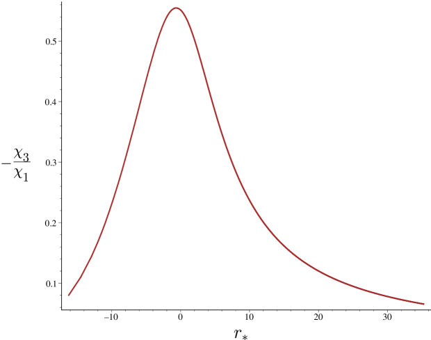
Figure 1: For a pure dipole background magnetic field this figure, which is a plot of Eq. (4-1), shows how the relative contributions from the interaction terms are dominated by $\chi_{1}$ (or $\chi_{2}$), except in the region just inside the photon sphere (the peak is at about $r\sim 2.4m$), where $\chi_{3}$ becomes significant (recall that $\chi_{3}$ is defined using the angular gradients of the radial part of the background magnetic field). The ‘tortoise’ coordinate $r_{*}$ is defined by Eq. (4-2) below.

The induced EM radiation will of course be of much higher amplitude far from the BH if we allow for the presence of the uniform magnetic field as part of the static background, as the interaction distance will be vastly increased. For the pure dipole magnetic field, the interaction distance is effectively curtailed at large $r$, because the magnetic field strength falls off so fast that $\mathscr{E}\gg\chi$ by $r\sim 20m$ or so. In astrophysical situations where the magnetic field extends far from the source (supported by an accretion disk, or entangled in the ejected envelope of the progenitor star, for example), we would expect further, linearly growing amplification, (beyond say $r\sim 20m$) over the amplification we report below. This will be studied at a later date when a plasma is included into the discussion, but should be borne in mind in what follows.

Hereafter we shall set $m=1$ (which just defines the units of $r$), and we shall use the tortoise coordinate $r_{*}$ of Regge and Wheeler (Regge and Wheeler, 1957) defined by

$${d\rho}=\tfrac{1}{2}\phi r{dr_{*}}=\left(\tfrac{1}{2}\phi r\right)^{-1}dr~{}~{}~{}\Rightarrow~{}~{}~{}r_{*}=r+2m\ln\left(\frac{r}{2m}-1\right).$$ (4-2)

Because the system of equations we are investigating are linear, the units we use are physically irrelevant, and is tied into the physical amplitude of our initial data which we normalise at unity (so that if units are chosen for $\chi$ say we can immediately read off the actual amplitudes for $\mathscr{E}$).

4.1 The initial value problem

Here we envisage the following situation: at some initial time $t=0$ the interaction is ‘turned on’ with some typical initial profile for the GW [i.e., the tensor $W_{ab}$, which translates in this case to $\bm{\chi}^{a}(t=0)=\bm{\chi}^{a}_{0}$], at which time the induced EM field is zero, but with non-zero second time derivatives (‘acceleration’). Although intuitively reasonable for modeling a situation such as BH formation or where the magnetic field becomes very strong very quickly, say, we require this switching on of the interaction because otherwise the ME will not be consistent for a general $\bm{\chi}^{a}_{0}$.

A common way of specifying initial data for this type of problem is to consider GW scattering off a BH, with the initial data given by a static narrow Gaussian peak at some distance from the hole (Andersson, 1997). This then splits in two as the RW equation is evolved, with the part falling into the hole of most interest: this scatters off the photon sphere and starts the black hole vibrating (roughly speaking), with a characteristic waveform which is largely independent of the initial data, dominated by the quasi-normal modes of the BH (which only depend on its mass) (Andersson, 1995, 1997; Sun and Price, 1998; Nollert, 1999). We will use this scenario with $W_{0}\sim\exp{\left(-(r_{*}-20)^{2}\right)}$ at $t=0$, which we normalise so that at $t=0$ and $r_{*}=20$, $\chi_{1_{\mathsf{V}}}=1$. We will not consider a pulse originating further from the hole because the dipole field falls off so fast with distance; the qualitative results remain the same.

We then evolve our key equation (3-41) and the wave equation for $\chi_{1}$ [modified by replacing $\chi_{3}$ with Eq. (4-1) as discussed above] with this initial data. This then gives the solution for $W_{\mathsf{S}}$, which we convert to $\mathscr{E}_{\mathsf{V}}$. Results are shown in Figs. (2) and (3) for $\log_{10}|\mathscr{E}_{\mathsf{V}}|$.

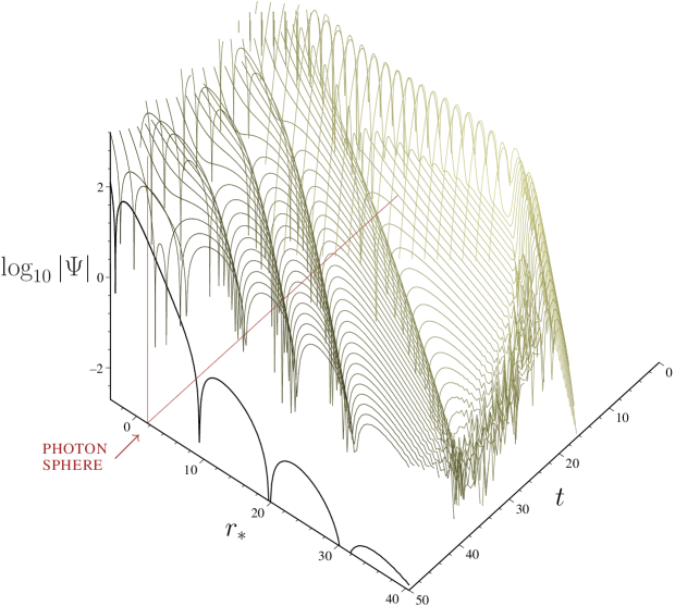
Figure 2: The induced EM radiation from static Gaussian initial data for the GW at $t=0$, such that the EM field is zero. This pulse splits into two, one falling into the hole and the other propagating to infinity. The part falling into the hole is partially reflected at about $t\sim 15$ generating the ‘ringing’ we see later at $t=50$ in the thick curve (modulated by the magnetic field here – this is $\chi_{1_{\mathsf{V}}}$). During this in-fall, the GW-B interaction produces substantial amounts of EM radiation which is reflected back away from the hole, and is further increased by the subsequent BH ringing.

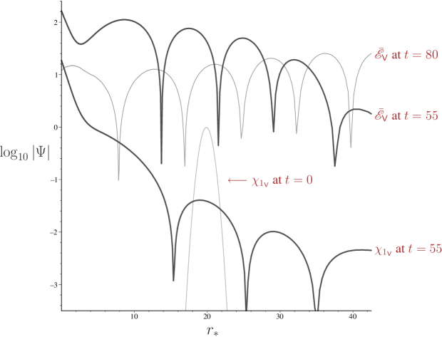
Figure 3: The induced EM radiation from static Gaussian initial data for the GW at $t=0$, such that $W\sim\exp{\left(-(r_{*}-20)^{2}\right)}$, normalised so that at $t=0$ and $r_{*}=20$, $\chi_{1_{\mathsf{V}}}=1$; at $t=0$ the EM field is zero. This pulse splits into two, one falling into the hole and the other propagating to infinity. The part falling into the hole is partially reflected generating the ‘ringing’ we see at $t=55$ (modulated by the magnetic field here in $\chi_{1_{\mathsf{V}}}$), in the wave which is moving to the right . During this in-fall, the GW-B interaction produces substantial amounts of EM radiation, which is further increased by the subsequent BH ringing. Thus we see at $t=55$ the EM field generated is two orders of magnitude larger than the initial pulse, and over three orders of magnitude larger than the interaction terms at the same distance from the hole. At $t=80$ we see that the main amplification has taken place with the peak of the induced EM radiation moving past $r_{*}\sim 40$.

These figures show the EM radiation generated and subsequently amplified during the scattering of the GW off the photon sphere. The ringing of the BH then generates a continuous stream of EM radiation, which at its peak is over two orders of magnitude larger than the initial pulse of radiation (by the time it is reflected back out to $r_{*}=20$). This radiation mirrors very closely the GW waveform making it a suitable EM counterpart for GW emission.

4.2 The quasi-normal mode approach

We shall now integrate the equations in the frequency domain, summing over the QNMs of the BH, which will tell us about the strength of the interaction in the latter stages of a perturbation of a BH independently of the initial perturbation (Andersson, 1997). We imagine that the interaction starts at $t=0$ at some inner radius $r_{0}$, so for $r<r_{0}$ we assume that $\mathscr{E}_{\mathsf{S}}=\beta_{\mathsf{S}}=0$, while $\bm{\chi}$ does its own thing; at $r=r_{0}$ we choose boundary conditions for each $\omega_{n}$ such that all EM terms and their derivatives are equal to zero; for want of accurate boundary conditions for the GW, we randomly choose $\bm{\chi}^{(\omega_{n})}=\bm{\chi}_{0}$. In order to compare differing amplifications for each parity, we use the same $\bm{\chi}_{0}$ for both parities. We then integrate Eqs. (3-45a) – (3-45) out to some $r=r_{\mbox{max}}$ for each QNM frequency $\omega_{n}$. Then, for each variable at $r=r_{\mbox{max}}$ we can simply add up the QNMs. This then gives a good approximation to the time decay of the signal as it passes $r=r_{\mbox{max}}$ after $t\mathrel{\vbox{\hbox{\tiny\ooalign{\raise 3.25pt\hbox{$>$}\crcr$\sim$}}}}t_{\mbox{max}}=r_{\mbox{max}}-r_{0}+2m\ln\left[\left(r_{\mbox{max}}-2m\right)/\left(r_{0}-2m\right)\right]$ (Andersson, 1997; Nollert, 1999). We use the first twelve QNM frequencies as tabulated in Nollert and Schmidt (1992) for $\sigma_{n}=\tfrac{1}{2}\phi r\omega_{n}$ – see Eq. (3-18).

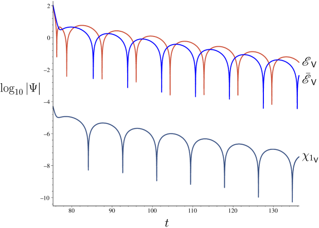
Figure 4: Late time behavior showing the temporal evolution of the generated EM waveforms for an observer at $r=65m$, using a quasi-normal mode expansion. Choosing boundary conditions at $r_{0}=2.05m$, the QNM sum will approximate the true solution for this observer after $t\simeq 76m$. We see that the EM waveform is substantially larger than the interaction variables, for which we have shown the largest, $\chi_{1_{\mathsf{V}}}$. The differing amplification of the electric field for each parity is also not insubstantial, with the even parity case being larger than the odd, in this case, demonstrating polarisation of the induced EM radiation.

In Figure 4 we show a typical result of this integration, for an observer situated at $r\simeq 65$, with $r_{0}=2.05$. The generated electric field is shown, for both parities, as is the largest interaction variable, which is $\chi_{1_{\mathsf{V}}}$ in this case. The units of the graph are arbitrary: dividing each variable by $|\bm{\chi}_{0}|$ (to make each variable dimensionless), say, will merely shift all the curves up or down. At large distances from the source, the behaviour of the fields can be represented as an amplitude over a potential of the distance function. In the case of the gravitational wave, the fall-off scales like $1/r$, while for a spherical electromagnetic wave it behaves as $1/r$. At the same time, the background magnetic dipole field has $1/r^{3}$-dependence. We can therefore normalise with the respect to the fall-off of the field strengths, in order to get a scale-invariant form of the amplification. In the situation given in Fig. 4, normalising the curve for $\chi_{1_{\mathsf{V}}}$ raises it up by $3\log_{10}\left(65/2.05\right)\sim 4.5$. Hence, at large distances from the source the scale-invariant amplification of the EM radiation is over two orders of magnitude larger the the magnitude of the GW times the magnetic field strength. At this distance from the source the interaction is no longer taking place to a significant degree, implying that this level of amplification is a generic feature. Note also from Fig. 4 that the amplification of the electric field parities is different, implying that the EM wave is polarised.

4.3 Estimates

To estimate the implications of this amplification we have found, consider the case of a compact object such as a BH or neutron star. The interaction between gravity waves and the magnetic field is quantified by the variable $\chi_{i}\sim h_{i}B_{i}$, where $h_{i}$ is the amplitude of the gravitational wave at the onset of the interaction, $B_{i}\sim B_{\text{s}}(r_{\text{s}}/r_{i})^{3}$ is the field strength at the distance $r_{i}$ from the compact object with ‘radius’ (e.g., surface of a neutron star or BH horizon) $r_{\text{s}}$ and surface magnetic field $B_{\text{s}}$. The interaction produces an EM signal $E_{\text{out}}$ which is typically two orders of magnitude larger at $r_{\text{cut-off}}$ than the original perturbation $\chi_{1}$ at $r_{\text{cut-off}}$, where the interaction effectively switches off. From Fig. 3 we extrapolate that at $r_{\text{cut-off}}\sim 40m$ we have roughly $\chi_{\text{cut-off}}\sim 10^{-2.5}\chi_{i}$, leading to an induced electric field strength

$$E_{\text{out}}\sim 3\times 10^{8}h_{i}\left(\frac{B_{\text{s}}}{1\,\mathrm{T}}\right)\left(\frac{r_{\text{s}}}{r_{i}}\right)^{3}\mathrm{Vm^{-1}}.$$ (4-3)

The induced signal attenuates inversely with distance $D$ outside the interaction region, e.g. $r\gtrsim 40m$. At a distance $D$ from the source, the spectral energy flux $\Phi_{\omega}=(\tfrac{1}{2}\epsilon_{0}cE^{2})/\omega$ can then be calculated to be

$$\Phi_{\omega}\sim 1.4\times 10^{6}h_{i}^{2}\left(\frac{B_{\text{s}}}{1\,\mathrm{T}}\right)^{2}\left(\frac{r_{\text{s}}}{r_{i}}\right)^{6}\left(\frac{r_{\text{cut-off}}}{100\,\mathrm{km}}\right)^{2}\left(\frac{10\,\mathrm{kpc}}{D}\right)^{2}\left(\frac{1\,\mathrm{kHz}}{\omega}\right)\mathrm{Jy}.$$ (4-4)

As an example, consider a magnetar of mass $m=1.5\,M_{\odot}$ with radius $r_{\text{s}}=9$ km, e.g. twice its Schwarzschild radius, and take $r_{i}=4\,r_{\text{s}}$ and $r_{\text{cut-off}}=90$ km, assuming a magnetic field strength $B_{\text{s}}$ in the range of $10^{5}$ to $10^{10}$ T. An occurring instability such as a supernova explosion or a bar mode instability is likely to produce a GW with $h_{i}\sim 10^{-3}$ and frequency $\omega$ of about $1-10$ kHz (Andersson, 2003), which is also the frequency of the induced EM wave. This leads to $E_{\text{out}}\sim 5\times 10^{8}-10^{13}\,\mathrm{Vm}^{-1}$. If such an event happened within our galaxy ($D\sim 10$ kpc), $\Phi_{\omega}\sim 10^{5}-10^{15}$ Jy, if we assume that 10% of the signal’s energy undergoes mode conversion shifting the frequency up to $30-300$ kHz (Marklund, Brodin, and Dunsby, 2000). To achieve a higher detection rate, one has to gather events from a farther distance. Events within the Virgo Cluster ($D\sim 15$ Mpc) would have flux $\Phi_{f}\sim 10^{-1}-10^{9}$ Jy. The proposed radio telescope Astronomical Low Frequency Array (Jones et al., 1998) is expected to operate in the range from 30 kHz to 30 MHz, with minimum detection level of 1000 Jy, making such events an exciting possibility for indirect gravitational wave detection.

5 Conclusions

We have investigated the scenario of GW around a Schwarzschild BH interacting with a strong, static, magnetic field. This interaction produces a stream of EM radiation mirroring the BH ringdown, with a stronger amplitude than one may expect from estimates of the interaction in flat space, due to non-linear amplification in the vicinity of the photon sphere. This interaction may play an important role in GRBs and perhaps some SN events, in addition to neutron star physics, and may be a useful mechanism to aid in GW detection.

We converted the Einstein-Maxwell equations into a linear, gauge-invariant system of differential equations by utilising the 1+1+2 covariant approach to perturbations of Schwarzschild. We also introduced a set of second order ‘interaction’ variables to aid in simplifying the derivation, and a new variable for the magnetic field, both of which made the system of equations manifestly gauge-invariant. It was then a simple matter to convert the system of equations into wave equations for integration as an initial value problem, or as a harmonically decomposed (in time) system of first-order ordinary differential equations, which could then be integrated using a BH quasi-normal mode expansion, an important approximation method for late time behaviour. We integrated the system of equations using both of these techniques.

A key point of this paper was to set up a suitable formalism to study this GW-B interaction around a BH, and to put the equations into a suitable gauge-invariant form for numerical integration. The next step is to include a plasma, as various plasma instabilities could be induced by such process, making detection of this sort of induced radiation a genuine possibility. This will also help model some of the relativistic effects which take place after a SN explosion. In fact, EM waves in a plasma in an exact Schwarzschild spacetime are pretty complicated and unexpected (Daniel and Tajima, 1997), so it is an interesting question in its own right to ask what happens when GW are thrown into the mix.

Appendix A Spherical harmonics

Here we briefly review the spherical harmonic expansion, developed in Clarkson and Barrett (2003) appropriate to the formalism, for easy reference. These allow us to remove all $\delta$-derivatives from the equations. Note that all functions and relations below are defined in the background only; we only expand second-order variables, or first-order variables which form part of a quadratic second-order variable so zeroth-order equations are sufficient.

We introduce spherical harmonic functions $Q=Q^{(\ell,m)}$, with $m=-\ell,\cdots,\ell$, defined on the background, such that

$$\delta^{2}Q=-\ell\left(\ell+1\right)r^{-2}Q,~{}~{}~{}\hat{Q}=0=\dot{Q}.$$ (A1)

We also need to expand vectors and tensors in spherical harmonics. We therefore define the even (electric) parity vector spherical harmonics for $\ell\geq 1$ as

$$Q_{a}^{(\ell)}=r\delta_{a}Q^{(\ell)}~{}~{}~{}\Rightarrow~{}~{}~{}\hat{Q}_{a}=0=\dot{Q}_{a},~{}~{}\delta^{2}Q_{a}=\left(1-\ell\left(\ell+1\right)\right)r^{-2}Q_{a};$$ (A2a)

where the $$(\ell)$$ superscript is implicit, and we define odd (magnetic) parity vector spherical harmonics as

$$\bar{Q}_{a}^{(\ell)}=r\varepsilon_{ab}\delta^{b}Q^{(\ell)}~{}~{}~{}\Rightarrow~{}~{}~{}\hat{\bar{Q}}_{a}=0=\dot{\bar{Q}}_{a},~{}~{}~{}\delta^{2}\bar{Q}_{a}=\left(1-\ell\left(\ell+1\right)\right)r^{-2}\bar{Q}_{a}.$$ (A2b)

Note that $\bar{Q}_{a}=\varepsilon_{ab}Q^{b}\Leftrightarrow Q_{a}=-\varepsilon_{ab}\bar{Q}^{b}$, so that $\varepsilon_{ab}$ is a parity operator. The crucial difference between these two types of vector spherical harmonics is that $\bar{Q}_{a}$ is solenoidal, so

$$\delta^{a}\bar{Q}_{a}=0,~{}~{}~{}\mbox{while}~{}~{}~{}\delta^{a}Q_{a}=-\ell\left(\ell+1\right)r^{-1}Q.$$ (A3)

Note also that

$$\varepsilon_{ab}\delta^{a}Q^{b}=0,~{}~{}~{}\mbox{and}~{}~{}~{}\varepsilon_{ab}\delta^{a}\bar{Q}^{b}=\ell\left(\ell+1\right)r^{-1}Q.$$ (A4)

The harmonics are orthogonal: $Q^{a}\bar{Q}_{a}=0$ (for each $\ell$). Similarly we define even and odd tensor spherical harmonics for $\ell\geq 2$ as

$$Q_{ab}=r^{2}\delta_{\{a}\delta_{b\}}Q,~{}~{}~{}\Rightarrow~{}~{}~{}\hat{Q}_{ab}=0=\dot{Q}_{ab},~{}~{}~{}\delta^{2}Q_{ab}=\left[\phi^{2}-3{\cal E}-\ell\left(\ell+1\right)r^{-2}\right]Q_{ab};$$ (A5a)

and

$$\bar{Q}_{ab}=r^{2}\varepsilon_{c\{a}\delta^{c}\delta_{b\}}Q,~{}~{}~{}\Rightarrow~{}~{}~{}\hat{\bar{Q}}_{ab}=0=\dot{\bar{Q}}_{ab},~{}~{}~{}\delta^{2}\bar{Q}_{ab}=\left[\phi^{2}-3{\cal E}-\ell\left(\ell+1\right)r^{-2}\right]\bar{Q}_{ab},$$ (A5b)

which are orthogonal: $Q_{ab}\bar{Q}^{ab}=0$, and are parity inversions of one another: $Q_{ab}=-\varepsilon_{c\{a}\bar{Q}_{b\}}^{~{}~{}c}\Leftrightarrow\bar{Q}_{ab}=\varepsilon_{c\{a}Q_{b\}}^{~{}~{}c}$.

We can now expand any second-order scalar ${\Psi}$ in terms of these functions as

$${\Psi}=\sum_{\ell=0}^{\infty}\sum_{m=-\ell}^{m=\ell}{\Psi}_{\mathsf{S}}^{(\ell,m)}Q^{(\ell,m)}={\Psi}_{\mathsf{S}}Q,$$ (A6)

where the sum over $\ell$ and $m$ is implicit in the last equality. The $\mathsf{S}$ subscript reminds us that ${\Psi}$ is a scalar, and that a spherical harmonic expansion has been made. Due to the spherical symmetry of the background, $m$ never appears in any equation so we can just ignore it. Any second-order vector ${\Psi}_{a}$ can now be written

$${\Psi}_{a}=\sum_{\ell=1}^{\infty}{\Psi}^{(\ell)}_{\mathsf{V}}Q_{a}^{(\ell)}+\bar{\Psi}^{(\ell)}_{\mathsf{V}}\bar{Q}_{a}^{(\ell)}={\Psi}_{\mathsf{V}}Q_{a}+\bar{\Psi}_{\mathsf{V}}\bar{Q}_{a}.$$ (A7)

Again, we implicitly assume a sum over $\ell$ in the last equality, and the $\mathsf{V}$ reminds us that ${\Psi}^{a}$ is a vector expanded in spherical harmonics. Any second-order tensor may be also be expanded

$${\Psi}_{ab}=\sum_{\ell=2}^{\infty}{\Psi}_{\mathsf{T}}^{(\ell)}Q_{ab}^{(\ell)}+\bar{\Psi}_{\mathsf{T}}^{(\ell)}\bar{Q}_{ab}^{(\ell)}={\Psi}_{\mathsf{T}}Q_{ab}+\bar{\Psi}_{\mathsf{T}}\bar{Q}_{ab}.$$ (A8)

Further useful identities are to be found in Clarkson and Barrett (2003).

References

- (1)
- Acernese et al. (2002) Acernese, F., et al. 2002, Class. Quantum Grav., 19, 1421
- Alcubierre (1998) Alcubierre, M., and Massó, J. 1998, Phys. Rev. D, 57, 4511
- Andersson (1995) Andersson, N. 1995, Phys. Rev. D, 51, 353
- Andersson (1997) Andersson, N. 1997, Phys. Rev. D, 55, 468
- Andersson (2003) Andersson, N. 2003, Class. Quantum Grav., 20, R105
- Ando et al. (2002) Ando, M., et al. 2002, Class. Quantum Grav., 19, 1409
- Barich and Weiss (1999) Barish, B., and Weiss, R. 1999, Phys. Today, 52, 44
- Brodin and Marklund (1999) Brodin, G., and Marklund, M. 1999, Phys. Rev. Lett., 82, 3012
- Brodin, Marklund, and Servin (2001) Brodin, G., Marklund, M., and Servin, M. 2001, Phys. Rev. D, 63, 124003
- Bruni et al. (1997) Bruni, M., Matarrese, S., Mollerach, S., and Sonego, S. 1997, Class. Quantum Grav., 14, 2585
- Bruni and Sonego (1999) Bruni, M., and Sonego, S. 1999, Class. Quantum Grav., 16, L29
- Buonanno (2002) Buonanno, A. 2002, Class. Quantum Grav., 19, 1267
- Cardoso et al. (2003) Cardoso, V., Lemos, J. P. S., and Yoshida, S. 2003, gr-qc/0307104
- Cardoso and Lemos (2003a) Cardoso, V. and Lemos, J. P. S. 2003, Phys. Rev. D, 67 084005
- Cardoso and Lemos (2003b) Cardoso, V. and Lemos, J. P. S. 2003, Gen. Rel. Grav., 35 L327
- Cardoso and Lemos (2002) Cardoso, V. and Lemos, J. P. S. 2002, Phys. Lett. B 538 1
- Chandrasekhar (1983) Chandrasekhar, S. 1983, The Mathematical Theory of Black Holes, Oxford: Oxford University Press
- Cooperstock (1968) Cooperstock, F. I. 1968, Ann. Phys., 47, 173
- Clarkson and Barrett (2003) Clarkson, C. A., and Barrett, R. K. 2003, Class. Quantum Grav., 20, 3855
- Daniel and Tajima (1997) Daniel, J., and Tajima, T. 1997, Phys. Rev. D, 55, 5193
- Ellis and Bruni (1989) Ellis, G. F. R., and Bruni, M. 1989, Phys. Rev. D, 40, 1804
- Ellis and van Elst (1998) Ellis, G. F. R., and van Elst, H. 1998, in Theoretical and Observational Cosmology, M. Lachieze-Rey (ed.), NATO Science Series, Kluwer Academic Publishers (gr-qc/9812046v4)
- Flanagan and Hughes (1998a) Flanagan, E. E., and Hughes, S. A. 1998a, Phys. Rev. D, 57 4535
- Flanagan and Hughes (1998b) Flanagan, E. E., and Hughes, S. A. 1998b, Phys. Rev. D, 57 4566
- Gerlach (1974) Gerlach, U. N. 1974, Phys. Rev. Lett., 32, 1023
- Jones et al. (1998) Jones, D. L., et al. 1998, in ASP Conf. Ser. 144 Radio Emission from Galactic and Extragalactic Compact Sources (eds.) Zensus J A, Taylor G B and Wrobel J M (San Francisco, ASP), 393
-
Kokkotas and Schmidt (1999)
Kokkotas,
K. D., and Schmidt, B. G. 1999, Living Rev. Relativity, 2, 2
(http://www.livingreviews.org/Articles/Volume2/1999-2kokkotas/) - Kouveliotou et al. (1998) Kouveliotou, C., et al. 1998, Nature, 393 235
- Macedo and Nelson (1983) Macedo, P. G., and Nelson, A. H. 1983, Phys. Rev. D, 28, 2382
- Marklund, Brodin, and Dunsby (2000) Marklund, M., Brodin, G., and Dunsby, P. K. S. 2000, ApJ, 536, 875
- Misner, Thorne, and Wheeler (1973) Misner, C. W., Thorne, K. S., and Wheeler, J. A. 1973, Gravitation, San Francisco: W. H. Freeman
- Mosquera Cuesta (2002) Mosquera Cuesta, H. J. 2002, Phys. Rev. D, 65, 064009
- Nicholson and Vecchio (1998) Nicholson, D., and Vecchio, A. 1998, Phys. Rev. D, 57, 4588
- Nollert (1999) Nollert, H-P. 1999, Class. Quantum Grav., 16, R159
- Nollert and Schmidt (1992) Nollert, H-P., and Schmidt, B. G. 1992, Phys. Rev. D, 45, 2617
- Price (1972) Price, R. H. 1972, Phys. Rev. D, 5, 2439
- Price and Pullin (1994) Price, R. H., and Pullin, J. 1994, Phys. Rev. Lett., 72, 3297
- Regge and Wheeler (1957) Regge, T., and Wheeler, J. A. 1957, Phys. Rev., 108, 1063
- Ruoff, Stavridis, and Kokkotas (2001) Ruoff, J., Stavridis, A., and Kokkotas, K. D. 2001, gr-qc/0109065; ibid, gr-qc/0203052
- Servin and Brodin (2003) Servin, M., and Brodin, G. 2003, Phys. Rev. D, 68, 044017
- Servin, Brodin, and Marklund (2001) Servin, M., Brodin, G., and Marklund, M. 2001, Phys. Rev. D, 64, 024013
- Stewart and Walker (1974) Stewart, J. M., and Walker, M. 1974, Proc. R. Soc. London A, 431, 49
- Sun and Price (1998) Sun, Y., and Price, R. H. 1988, Phys. Rev. D, 38, 1040
- Sylvestre (2003) Sylvestre, J. 2003, ApJ, 591, 1152
- Thorne (1980) Thorne, K. S. 1980, Rev. Mod. Phys., 52, 299
- van Putten (2001) van Putten, M. 2001, Phys. Rev. Lett., 87, 091101
- Willke et al. (2002) Willke, B., et al. 2002, Class. Quantum Grav., 19, 1377