Evolution of Planetary Systems in Resonance

We study the time evolution of two protoplanets still embedded in a protoplanetary disk. The results of two different numerical approaches are presented and compared. In the first approach, the motion of the disk material is computed with viscous hydrodynamical simulations, and the planetary motion is determined by N-body calculations including exactly the gravitational forces exerted by the disk material. In the second approach, only the N-body integration is performed but with additional dissipative forces included such as to mimic the effect of the disk torques acting on the disk. This type of modeling is much faster than the full hydrodynamical simulations, and gives comparative results provided that parameters are adjusted properly.

Resonant capture of the planets is seen in both approaches, where the order of the resonance depends on the properties of the disk and the planets. Resonant capture leads to a rise in the eccentricity and to an alignment of the spatial orientation of orbits. The numerical results are compared with the observed planetary systems in mean motion resonance (Gl 867, HD 82943, and 55 Cnc). We find that the forcing together of two planets by their parent disk produces resonant configurations similar to those observed, but that eccentricity damping greater than that obtained in our hydrodynamic simulations is required to match the GJ 876 observations.

1 Introduction

Since their first discovery in 1995, the number of detected extrasolar planets orbiting solar-type stars has risen during recent years to more than 100 (for an up-to-date list see e.g. http://www.obspm.fr/encycl/encycl.html by J. Schneider). Among these, there are currently 11 systems with two or more planets; a summary of their properties has been given recently by Marcy et al. (2003). With further observations to come, the fraction of systems with multiple planets will almost certainly increase, as many of the systems exhibit long-term trends in their radial velocity, suggesting an additional outer planet. Among the known multiple-planet extrasolar systems there are now three confirmed cases, namely Gl 876 (Marcy et al. 2001), HD 82943 (the Coralie Planet Search Programme, ESO Press Release 07/01), and 55 Cnc (Marcy et al. 2002) where the planets orbit their central star in a low-order mean motion resonance such that the orbital periods have nearly exactly the ratio 2:1 or 3:1. The parameters of these planetary systems are displayed in Table 1 below. The possibility of a 2:1 resonance in HD 160691 has also been discussed recently by Bois et al. (2003), although the orbital periods are too long to definitely confirm this. Overall, these numbers imply that at least one-fourth of multiple-planetary systems contain planets in resonance, a fraction which is even higher if secular resonances, such as those observed in the $\upsilon$ And system, (Butler et al. 1999) are also considered.

The formation of resonant planetary systems can be understood by considering the joint evolution of protoplanets together with the protoplanetary disk from which they formed. Using local linear analysis, it has been shown that the gravitational interaction of a single protoplanet with its disk leads to torques resulting in a change of the semi-major axis (migration) of the planet (Goldreich & Tremaine 1980; Lin & Papaloizou 1986; Ward 1997; Tanaka et al. 2002). Additionally, as a result of angular momentum transfer between the viscous disk and the planet, planetary masses of around one Jupiter mass can open gaps in the surrounding disk (Lin & Papaloizou 1980, 1993). Fully non-linear hydrodynamical calculations for Jupiter-sized planets (Kley 1999; Bryden et al. 1999; Lubow et al. 1999; Nelson et al. 2000; D’Angelo et al. 2002) confirmed this expectation and clearly showed that disk-planet interaction leads to: i) excitation of spiral shock waves in the disk, whose tightness depends on the sound-speed in the disk, ii) formation of an annular gap, whose width is determined by the balance between gap-opening tidal torques and gap-closing viscous plus pressure forces, iii) inward migration on a time scale of $10^{5}$ yrs for typical disk parameters, in particular disk masses corresponding to that of the minimum mass solar nebula, iv) possible mass growth after gap formation up to about 10 $M_{Jup}$ when finally the gravitational torques overwhelm the diffusive tendencies of the gas, and v) a prograde rotation of the planet. New three-dimensional computations with high resolution resolve the flow structure in the vicinity of the planet, and allow for more accurate estimates of the mass accretion and migration rates (D’Angelo et al. 2003; Bate et al. 2003).

These hydrodynamic simulations with single planets have been extended to models which contain multiple planets. It has been shown (Kley 2000; Bryden et al. 2000; Snellgrove et al. 2001; Nelson & Papaloizou 2002) that during the early evolution, when the planets are still embedded in the disk, different migration speeds may lead to an approach of neighboring planets and eventually to resonant capture. More specifically, the evolution of planetary systems into a 2:1 resonant configuration was seen in the calculations of Kley (2000) prior to the discovery of any such systems.

In addition to hydrodynamic disk-planet simulations, many authors have analyzed the evolution of multiple-planet systems with N-body methods. Each of the known resonant systems have been considered in detail. Ji et al. (2002) and Lee & Peale (2002a) have modeled the evolution of 2:1 resonant system GJ 876, while the 3:1 system 55 Cnc has been analyzed by Ji et al. (2003b) and Lee & Peale (2002b), and the 2:1 system HD 82943 by Goździewski & Maciejewski (2001) and Ji et al. (2003a). Based on orbit integrations, these papers confirm that the planets in these systems are in resonance with each other. The dynamics and stability of resonant planetary systems in general has been recently studied by Beauge et al. (2002).

Here we present new numerical calculations treating the evolution of two planets still embedded in a protoplanetary disk. We use both hydrodynamical simulations and simplified N-body integrations to follow the evolution of the system. In the first approach, the disk is evolved by solving the full time-dependent Navier-Stokes equations simultaneously with the evolution of the planets. Here, the motion of the planets is determined by the gravitational action of both planets, the star, and the disk. In the latter approach, we take a simplified approximation and perform 3-body (star plus two planets) calculations augmented by additional (damping) forces which approximately account for the gravitational influence of the disk (e.g. Lee & Peale 2002a). Using both approaches, allows a direct comparison of the alternative methods, and does enable us to determine the damping parameters required for the simpler (and much faster) second type of approach.

2 The Observations

The basic orbital parameters of the three known systems in mean motion resonance are presented in Table 1. The orbital parameters for Gl 876 are taken from the dynamical fit of Laughlin & Chambers (2001), and for HD 82943 from Goździewski & Maciejewski (2001). Due to the uncertainty in the inclinations of the systems, $M\sin i$, rather than the exact mass of each planet, is listed. By including the mutual perturbations of the planets into their fit of Gl 876, Laughlin & Chambers (2001), however, are able to constraint that system’s inclination to $\sim 30^{o}-50^{o}$.

Two of the systems, Gl 876 and HD 82943, are in a nearly exact 2:1 resonance. We note that in both cases the outer planet is more massive, in one case by a factor of about two (HD 82943) and in the other by more than three (Gl 876). The eccentricity of the inner (less massive) planet is larger than that of the outer one in both systems. For the system Gl 876 the alignment of the orbits is such that the two periastrae are pointing in nearly the same direction. For the system HD 82943 these data have not been clearly identified, due to the much longer orbital periods, but they do not seem to be very different from each other. The third system, 55 Cnc, is actually a triple system. Here the inner two planets orbit the star very closely and are in a 3:1 resonance, while the third, most massive planet orbits at a distance of several AU.

Table 1: The orbital parameters of the three systems known to contain a mean motion resonance. $P$ denotes the orbital period, $M\sin i$ the mass of the planets, $a$ the semi-major axis, $e$ the eccentricity, ${\varpi}$ the angle of periastron, and $M_{*}$ the mass of the central star. It should be noted that the orbital elements for shorter period planets undergo secular time variations. Thus in principle one should always state the epoch corresponding to these osculating elements (see e.g. Laughlin & Chambers 2001).

Name	P	$M\sin i$	a	$e$	${\varpi}$	$M_{*}$
	[d]	[$M_{Jup}$]	[AU]		[deg]	[$M_{\odot}$]
Gl 876	(2:1)					0.32
c	30.1	0.56	0.13	0.24	159
b	61.02	1.89	0.21	0.04	163
HD 82943	(2:1)					1.05
b	221.6	0.88	0.73	0.54	138
c	444.6	1.63	1.16	0.41	96
55 Cnc	(3:1)					0.95
b	14.65	0.84	0.11	0.02	99
c	44.26	0.21	0.24	0.34	61
d	5360	4.05	5.9	0.16	201

3 The Models

Our goal is to investigate the evolution of protoplanets still embedded in their disk. As outlined in the introduction, we employ two different methods which complement each other. First, a fully time-dependent hydrodynamical model for the joint evolution of the planets and disk is presented. Because the evolutionary time scale may cover several thousands of orbits, the fully hydrodynamical computations (of disk and planets) can require millions of time-steps, which translates into an effective computational time of up to several weeks.

Since our main interest is the orbital evolution of the planets and not so much the hydrodynamics of the disk, we also perform 3-body orbit integrations which do not explicitly follow the disk’s evolution. Through a direct comparison with the hydrodynamical models, it is then possible to infer the effective damping forces to include within this faster calculation.

3.1 Hydrodynamical Model

The first set of coupled hydrodynamical-N-body models presented in this paper are calculated in the same manner as the models described previously in Kley (1998, 1999) for single planets and in Kley (2000) for multiple planets. The reader is referred to those papers for details on the computational aspects of the simulations. Other similar models, following explicitly the motion of single and multiple planets in disks, have been presented by Nelson et al. (2000), Bryden et al. (2000), and Snellgrove et al. (2001).

3.1.1 Equations

For reference, we summarize the basic equations for this problem. We use two-dimensional cylindrical coordinates ($r,\varphi$), where $r$ is the radial coordinate and $\varphi$ is the azimuthal angle. Thus, we consider an infinitesimally thin disk located at $z=0$, with a velocity field ${\bf u}=(u_{r},u_{\varphi})$. The origin of the coordinate system is at the position of the star. In the following we will use the symbol $v=u_{r}$ for the radial velocity and $\omega=u_{\varphi}/r$ for the angular velocity of the flow. As there is no preferred rotational frame, we work in a non-rotating reference system. Then the equations of motion are

$$\frac{\partial\Sigma}{\partial t}+\nabla\cdot(\Sigma{\bf u})=0,$$ (1)

$$\frac{\partial(\Sigma v)}{\partial t}+\nabla\cdot(\Sigma v{\bf u})=\Sigma\,r\omega^{2}-\frac{\partial p}{\partial r}-\Sigma\frac{\partial\Phi}{\partial r}+f_{\mathrm{r}}$$ (2)

$$\frac{\partial(\Sigma r^{2}\omega)}{\partial t}+\nabla\cdot(\Sigma r^{2}\omega{\bf u})=-\frac{\partial p}{\partial\varphi}-\Sigma\frac{\partial\Phi}{\partial\varphi}+f_{\mathrm{\varphi}}$$ (3)

Here $\Sigma$ denotes the surface density, $p$ the two-dimensional pressure, and $f_{r},f_{\varphi}$ denote the components of the viscous forces, given explicitly in Kley (1999). The gravitational potential $\Phi$ generated by the protostar with mass $M_{*}$ and the two planets having mass $m_{1}$ and $m_{2}$ is given by

$$\Phi=-\frac{GM_{*}}{|{\bf r}-{\bf r}_{*}|}-\frac{Gm_{1}}{\left[({\bf r}-{\bf r}_{1})^{2}+s_{1}^{2}\right]^{1/2}}-\frac{Gm_{2}}{\left[({\bf r}-{\bf r}_{2})^{2}+s_{2}^{2}\right]^{1/2}}$$ (4)

where $G$ is the gravitational constant and ${\bf r}_{*}$, ${\bf r}_{1}$, and ${\bf r}_{2}$ are the position vectors for the star and the inner/outer planet, respectively. The quantities $s_{1}$ and $s_{2}$ are smoothing lengths that are set to 1/5 of each planet’s Roche radius. This softening of the potential removes any local fluctuations that might result as the planets move through the computational grid.

The motion of the star and the planets is determined firstly by their mutual gravitational interaction and secondly by the gravitational forces exerted upon them by the disk. The acceleration of the star ${\bf a}_{*}$ is given for example by

$${\bf a}_{*}=Gm_{1}\frac{{\bf r}_{1}-{\bf r}_{*}}{|{\bf r}_{1}-{\bf r}_{*}|^{3}} + Gm_{2}\frac{{\bf r}_{2}-{\bf r}_{*}}{|{\bf r}_{2}-{\bf r}_{*}|^{3}}$$ (5)

$$+ G\int_{Disk}\Sigma(r,\varphi)\,\frac{{\bf r}-{\bf r}_{*}}{|{\bf r}-{\bf r}_{*}|^{3}}\,dA$$

where the integration covers the entire disk surface. The accelerations of the planets are found similarly. We work here in an accelerated coordinate frame where the origin is located in the center of the (moving) star. Thus, in addition to force due to the gravitational potential (Eq. 4), the disk and planets also feel an acceleration $-{\bf a}_{*}$.

3.1.2 Initial and boundary conditions

The initial hydrodynamic structure of the disk, which extends radially from $r_{min}$ to $r_{max}$, is axisymmetric with respect to the location of the star, and the surface density scales as $\Sigma(r)=\Sigma_{0}\,r^{-1/2}$, with superimposed initial gaps (Kley 2000). The initial velocity is pure Keplerian rotation ($v_{r}=0,v_{\varphi}=GM_{*}/r^{1/2}$). We assume a fixed temperature law with $T(r)\propto r^{-1}$ which follows from the assumed constant vertical height $H/r$. The kinematic viscosity $\nu$ is typically parameterized by an $\alpha$-description $\nu=\alpha c_{s}H$, with the sound speed $c_{s}=Hv_{\varphi}/r$, only one model (X) has a constant kinematic viscosity.

The radial outer boundary is closed, i.e. $v_{r}(r_{max})=0$. At the inner radial boundary outflow boundary conditions are applied; matter may flow out, but none is allowed to enter. This procedure mimics the accretion process onto the star. The density gradient is set to zero at $r_{min}$ and $r_{max}$, while the angular velocity there is fixed to be Keplerian. In the azimuthal direction, periodic boundary conditions for all variables are imposed.

3.1.3 Model parameters

We present several models that are listed in Table 2, for the complete model parameters see below. In all cases, the planets are allowed to migrate (change their semi-major axes) through the disk in accordance with the gravitational torques exerted on them. During the evolution, material is removed from the centers of the planets’ Roche-lobes and is assumed to have been accreted onto each planet, for the detailed procedure see Kley (1999). However, in spite of this assumed accretion process, in most models this mass is not added to the dynamical mass of the planets. Hence, the disk mass is slowly depleted while the planets’ masses are held fixed at the initial values. This assumption of constant planet mass throughout the computation is well justified, as the migration rate depends only weakly on the mass of the planet (Nelson et al. 2000). Only in the last model X are the masses of the planets allowed to grow during the computation, which may test this assumption.

Table 2: Planetary and disk parameters of the hydrodynamic models. The masses of the planets are given in Jupiter masses ($M_{Jup}=10^{-3}M_{\odot}$). Index 1 refers to the inner and index 2 to the outer planet. For the last model X, we allow for variable planet masses which both start with 1 $M_{Jup}$ and then grow during the computation. For the viscosity, the corresponding value of $\alpha$ is given except for the last case (model X) in which we use a constant kinematic viscosity (corresponding to $\alpha=0.04$ at a radial location of $5.2$ AU). The relative disk scale height $H/r$ is given in the last column. For the disk masses and computational domains, see section 3.1.

Model	$m_{1}$	$m_{2}$	Viscosity	$H/r$
	[$M_{Jup}$]	[$M_{Jup}$]	$\alpha$
A	5	3	$10^{-2}$	0.10
B	5	3	$2\cdot 10^{-3}$	0.10
C	3	5	$10^{-2}$	0.10
D1, D2	3	5	$3\cdot 10^{-3}$	0.10
E	3	5	$10^{-3}$	0.10
F	3	5	$10^{-2}$	0.075
G	3	5	$10^{-2}$	0.05
X	1 (V)	1 (V)	$\nu=const.$	0.05

In all the models A-G, the disk extends radially from $r_{min}=1$ to $r_{max}=30$ AU. The disk mass within this radial range is about 0.04 $M_{\odot}$, and the planets are always placed initially at 4 and 10 AU, respectively. In the first two models (A & B), the inner planet is more massive than the outer one, while in models C through G the inner planet is less massive. A range of values for the viscosity and disk thickness $H/r$ are considered, as listed in Tab. 2. The values of $\alpha=0.01$ and $H/r=0.1$ may be on the high side for protoplanetary disks but allow for a sufficiently rapid evolution of the system to identify clearly the governing physical effects. The influence of these parameters is studied by comparison between different models. The parameters for models D1 and D2 are identical, but in the second case the density has been perturbed randomly by 1%.

Model X differs in several respects from the other models. The kinematic viscosity $\nu$ is constant and equivalent to $\alpha=0.004$ at 5.2 AU. Here, both embedded planets each have initial masses of 1 $M_{Jup}$ and are placed initially at 1 and 2 AU. This model is a continuation of the one presented previously in Kley (2000). The radial extent of the disk for this model was $r_{min}=1.3$ to $r_{max}=20.8$ AU, which contained a disk mass of $0.01M_{\odot}$ initially. The initial setup makes the surface density $\Sigma(r)$ the same for all models.

3.2 Damped N-body Model

As pointed out, the full hydrodynamical evolution is computationally very time consuming since tens of thousands of orbits must be calculated. Hence, we also perform simpler N-body calculations of planetary systems with two planets orbiting a single star. We consider only coplanar systems, where the planetary orbits and the equatorial plane of the disk are all aligned. The orbit of a single planet around a star is an ellipse and is determined by three orbital elements: the semi-major axis $a$, the eccentricity $e$, and the direction of periastron ${\varpi}$. The actual location of the planet within the orbit can be obtained from the elapsed time since last periastron. In the case of a planetary system with more than one planet, due to the mutual gravitational perturbations the ellipses are no longer fixed in space. In the case where the masses of the planets are much smaller that the stellar mass, at each epoch we can fit an instantaneous ellipse to the orbit of each planet and obtain the corresponding osculating elements of the orbit. These are calculated for each planet individually, considering only one planet at a time.

The gravitational influence of the surrounding disk is modeled here through prescribed (damping) forces. We assume that these forces act on the momentary semi-major axis and eccentricity of the planets through explicitly specified relations for $\dot{a}(t)$ and $\dot{e}(t)$, which vary with time. The changes $\dot{a}$ and $\dot{e}$ caused by the damping effects of the disk can be translated into additional forces changing directly the position ${\@vec{x}}$ and velocity ${\@vec{u}}$ of the planets. Our implementation follows Lee & Peale (2002a), where explicit expressions for these damping terms are given. As a test, we recalculated their model for GJ 876 and confirmed their results.

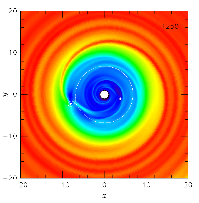
Figure 1: Overview of the density distribution of model C after 1500 orbital periods of the inner planet. Higher density regions are brighter and lower ones are darker. The star lies at the center of the white inner region bounded by $r_{min}=1$ AU. The location of the two planets is indicated by the white dots, and their Roche-lobes are also drawn. Clearly seen are the irregular spiral wakes generated by the planets. Regular intertwined spiral arms are seen only outside of the second planet.

Motivated by the basic idea of two planets orbiting inside a disk’s cavity (see Fig. 1), we damp $a$ and $e$ for the outer planet only. We adopt a logarithmic time derivative of $a$ of the form

$$\frac{\dot{a}}{a}=-\frac{1}{\tau(t)}\,\qquad\mbox{with}\qquad\,\tau(t)=\,\tau_{0}\,+\,\beta t,$$ (6)

where $\tau(t)$ denotes the damping time, and $\beta$ a dimensionless positive ’stretching’ constant. By making the ansatz Eq. (6) we tried to make the damping as simple as possible with only two parameters to fit. In practice we found that the damping time $\tau$ could not be chosen as a fixed constant, such that we assume a simple linear time dependence. Equation (6) can be integrated to yield

$$a(t)=a_{0}\cdot\left(1\,+\,\beta\,\frac{t}{\tau_{0}}\right)^{-1/\beta},$$ (7)

where ${a}_{0}$ denotes the starting value of $a$ at the initial time $t_{0}=0$.

The eccentricity damping is set to a fixed multiple of the semi-major axis damping

$$\frac{\dot{e}}{e}=K\,\,\frac{\dot{a}}{a},$$ (8)

where $K$ is a constant, typically larger than unity (see also Lee & Peale 2002a).

The time scale $\tau_{0}$, the ’stretching’ factor $\beta$, and $K$ are adjusted in order to match the results of the full hydrodynamic calculations. Results of the two methods are compared in Section 4.2 below.

4 Results

The basic evolutionary sequence of two planets evolving simultaneously with a hydrodynamic disk has been calculated and described by Kley (2000) and Bryden et al. (2000). The model X was considered in Kley (2000), where it was found that both planets evolve into a 2:1 resonant configuration. Model X and model A are discussed further in a recent conference paper Kley (2003). Here, these models are listed essentially for completeness, while our main interest in this paper focuses on models C-G.

To analyze the system dynamics in the presence of a disk, we monitor the evolution of the orbital elements $a$, $e$, and ${\varpi}$ of both planets throughout the simulations. In the case of a resonance, the orbits are coupled dynamically. For coplanar systems that are in a mean-motion commensurability $(p+q)$:$p$, it suffices to use two resonant angles to describe the evolution. Here we consider the angular difference of the apsidal lines

$$\Delta{\varpi}={\varpi}_{2}-{\varpi}_{1}$$ (9)

and the combination

$$\Theta_{1}=(p+q)\lambda_{2}-p\lambda_{1}-q{\varpi}_{1},$$ (10)

where $\lambda_{i}$ are the mean longitudes of the inner ($i=1$) and outer ($i=2$) planets. The two resonant angles $\Delta{\varpi}$ and $\Theta_{1}$ have also been used recently by Beauge et al. (2002) to study the possible stable solutions of resonant planetary systems. In Eq. (10), we have $p=1$, $q=1$ for a 2:1 resonance, while for a 3:1 resonance $p=1$, $q=2$.

Before we discuss details of resonant planetary evolution we briefly summarize the main properties of model C, which serves as our standard reference model.

4.1 Hydrodynamical Models

4.1.1 Overview

At the start of the simulations both planets are placed into an axisymmetric disk, where the density is initialized with partially opened gaps superimposed on an otherwise smooth radial density profile. Upon starting the evolution the two main effects are:

1. Because of the accretion of gas onto the two planets the radial region in between them is depleted in mass and finally cleared. This clearing time depends on the mass of the planets and on the viscosity and temperature of the disk. The individual gaps of higher mass planets are deeper, which lengthens the overall clearing timscale. Higher viscosity and temperature tend to ’push’ material towards the planets and shorten the clearing time. Additionally, the disturbance by the two planets creates a strongly time dependent flow with two mutually interacting spiral arms which also pushes matter towards the planets. The snapshot in Fig. 1 shows clearly this effect, which again reduces the clearing time. Thus, the high viscosity ($\alpha=0.01$) and temperature ($H/R=0.1$) of the standard model (C) still allow for gap clearing in spite of the large mass of the planets. After about 5000 yrs, only 2% of the initial material between the planets remains. For model X, with lower mass planets, this phase takes only a few hundred orbital periods (Kley 2000).

   Concurrently with the central ring depletion, the region interior to the inner planet loses material either due to accretion onto the central star (the inner boundary is open to outflow) or by accretion onto the planet. As with the intermediate ring, the timescale for clearing this inner region again depends on the physical parameter of the system. Thus, after an initial transient phase we typically expect the configuration of two planets orbiting within an inner cavity of the disk, as seen in Fig. 1 (see also Kley 2000).

2. After initialization, the planets quickly (within a few orbital periods) excite non-axisymmetric disturbances, viz. the spiral waves, in the disk. In contrast to the single planet case these are not stationary in time, because there is no preferred rotating frame. The gravitational torques exerted on the two planets by those non-axisymmetric density perturbations induce a migration process for the planets.

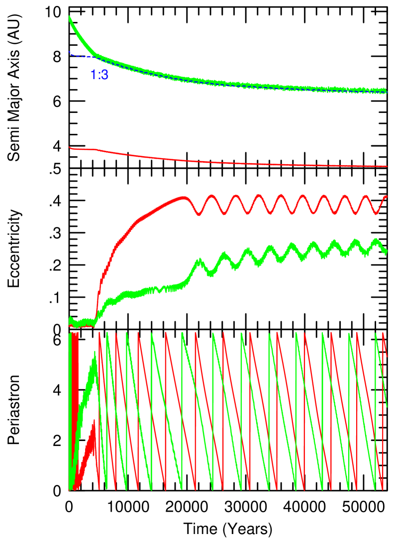
Figure 2: The semi-major axis ($a$), eccentricity ($e$) and position angle of the orbital periastron (${\varpi}$) for the two planets versus time for Model C. In this example, the planets have fixed masses of 3 and 5 $M_{Jup}$, and are placed initially at 4 and 10 AU, respectively. The inner planet is denoted by the black line, the outer by the light gray line. The dotted reference line (labeled 3:1), indicates the location of the 3:1 resonance with respect to the inner planet.

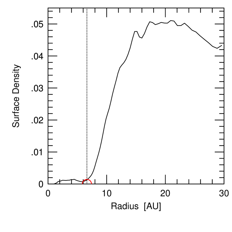
Figure 3: The azimuthally averaged surface density (in dimensionless units) for model C at 40,000 yrs. The location of the semi-major axis of the planet is indicated by the vertical dashed line at $r=6.63$, and the size of its Roche-radius by the solid circle. The left and right arrows indicate the locations of the inner and outer 2:1 Lindblad resonances, respectively.

Now, the planets’ relative positions within the cavity have a distinct influence on their subsequent evolution. As a consequence of the clearing process, the inner planet is no longer surrounded by any disk material and thus cannot grow any further in mass. In addition, it cannot migrate anymore, because there is no torque-exciting material left in its vicinity. All the material of the outer disk is still available, on the other hand, to exert negative (Lindblad) torques on the outer planet. Hence, in the initial phase of the computations we observe an inwardly migrating outer planet and a stalled inner planet with a constant semi-major axis (see the first 5000 yrs in the top panel of Fig. 2).

During the inward migration process the eccentricity of the outer planet remains small. As can be seen from Fig. 3 there is always a sufficient amount of matter in the immediate vicinity (co-orbital region) of the planet to ensure damping of the eccentricity. For a 5 Jupiter mass planet at $r=6.63$AU the Roche-lobe size is $0.78$ AU, which is indicated by the radius of the drawn circle. The arrows denote the position of the inner and outer 2:1 Lindblad resonances.

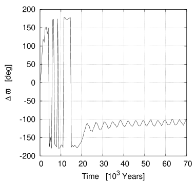
Figure 4: Evolution of $\Delta{\varpi}$ and $\Theta_{1}$ in model C. Left: The difference in the direction of the periastrae, $\Delta{\varpi}={\varpi}_{2}-{\varpi}_{1}$ (in degrees) for both planets versus time (in thousand years). Right: The resonant angle for the 3:1 resonance $\Theta_{1}=3\lambda_{2}-\lambda_{1}-2{\varpi}_{1}$ (in degrees) as a function of time.

The decrease in separation between the planets increases their gravitational interactions. Once the ratio of the planets’ orbital periods has reached a ratio of two integers, i.e. they are close to a mean motion resonance, resonant capture of the inner planet by the outer one may ensue. Whether or not this does actually happen depends on the physical conditions in the disk (e.g. viscosity) and the orbital parameters of the planets. If the migration speed is too large, for example, there may not be enough time to excite the resonance, and the outer planet will continue migrating inward (e.g. Haghighipour 1999). Also, if the initial eccentricities are too small, then there may be no capture, particularly for second-order resonances such as the 3:1 resonance (see e.g. Murray & Dermott 1999). For more details on capture probability see section (4.3.3) below.

4.1.2 3:1 Resonance: Model C

The typical time evolution of the semi-major axis ($a$), eccentricity ($e$) and direction of the periastron (${\varpi}$) are displayed in Fig. 2 for the standard model C. The planets were initialized with zero eccentricities at distances of 4 and 10 AU in a disk with partially cleared gaps.

In the beginning, after the inner gap has completely cleared, only the outer planet migrates inward, and the eccentricities of both planets remain relatively small, ($\lower 3.0pt\hbox{${\buildrel<\over{\sim}}$}\ 0.02$). After about 5000 yrs the outer planet has reached a semi-major axis with an orbital period three times that of the inner planet. The periodic gravitational forcing leads to the capture of the inner planet into a 3:1 resonance with the outer one. This is indicated by the dotted reference line (labeled 3:1) in the top panel of Fig. (2), which marks the location of the 3:1 resonance with respect to the inner planet.

We summarize the following important features of the evolution after resonant capture:

1. In the course of the subsequent evolution, the outer planet, which is still driven inward by the outer disk material, forces the inner planet to also migrate inwards. Both planets migrate inward simultaneously, always retaining their resonant configuration. Consequently, the migration speed of the outer planet slows down, and their radial separation declines.

2. Upon resonant capture the eccentricities of both planets grow initially very fast before settling into an oscillatory quasi-static state which changes slowly on a secular time scale. This slow increase of the eccentricities on the longer time scale is caused by the growing gravitational forces between the planets, due to the decreasing radial distance of the two planets on their inward migration process.

3. The ellipses/periastrae of the planets rotate at a constant, retrograde angular speed $\dot{{\varpi}}$. Coupled together by the resonance, the apsidal precession rate $\dot{{\varpi}}$ for both planets is identical, which can be inferred from the parallel lines in the bottom panel of Fig. 2. The orientation of the orbits is phase-locked with a constant separation $\Delta{\varpi}={\varpi}_{2}-{\varpi}_{1}$. The rotation period of the ellipses (apsidal lines) is slightly longer than the oscillation period of the eccentricities.

Figure 5: Eccentricity ratio $e_{2}/e_{1}$ of the outer and inner planet, versus periastron difference $\Delta{\varpi}$ for model C. The data points are spaced equally in time with a distance of approximately $\delta t=23$ yrs. Shown is a section of the evolution of model C, from 26,000 to 55,000 yrs, which covers about 7 libration periods.

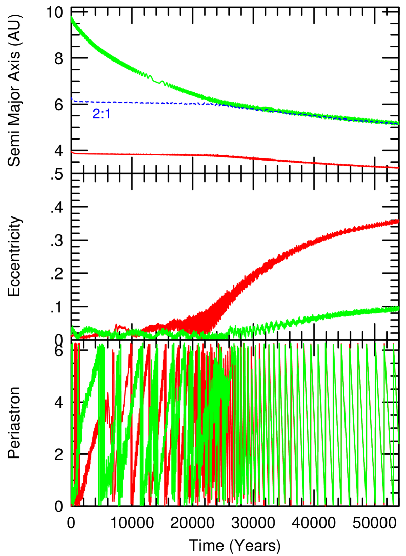
Figure 6: The semi-major axis, eccentricity and position angle of the orbital periastron versus time for Model D. The only parameter different from the first model C is the lower viscosity. Here, the outer planet passes through the 3:1 resonance and captures the inner planet finally into a 2:1 configuration. The dotted reference line (labeled 2:1) marks the location of the 2:1 resonance with respect to the inner planet. Upon resonant capture, the eccentricities grow and the two orbits librate retrograde with a fixed relative orientation of $\Delta{\varpi}=0^{o}$.

The capture into resonance and the subsequent libration of the orbits in model C is illustrated further in Fig. 4. As suggested in Fig. 2 (bottom panel) the periastrae begin to align upon capture in the 3:1 resonance. Initially, during the phase when the eccentricities are still rising (between 5 and 20 thousand yrs), the difference of the periastrae settles intermediately to $\Delta{\varpi}\approx 180^{o}$ (see Fig. 4, left panel). Then, upon saturation after about 20,000 yrs, the system re-adjusts and eventually establishes itself at $\Delta{\varpi}\approx 107^{o}$, with a libration amplitude of about $7^{o}$. The right panel of Fig. 4 shows the time evolution of the resonant angle $\Theta_{1}=3\lambda_{2}-\lambda_{1}-2{\varpi}_{1}$. Here $\lambda_{1}$ and $\lambda_{2}$ denote the mean longitudes of the inner and outer planet, respectively. Initially, $\Theta_{1}$ settles to $180^{o}$ as well, and re-adjusts after 20,000 yrs to $-145^{o}$ with a libration amplitude of $\pm 15^{o}$. This behavior of an initially symmetric alignment of $\Delta{\varpi}$ and $\Theta_{1}$ at about $180^{o}$ followed by a later change to $\Delta{\varpi}\approx\pm 110^{o}$ and $\Theta_{1}\approx\pm 145^{o}$ is characteristic for all our models which show captures into 3:1 resonance, independent of the physical parameters (see Tab. 4).

This behavior can be understood by an analysis of the interaction Hamiltonian for resonant systems (Beauge et al. 2002). By minimizing the interaction energy, the equilibrium values for $\Delta{\varpi}$ and $\Theta_{1}$ can be obtained as a function of the mass and eccentricity of the two planets. As shown by Beauge et al. (2002), when the eccentricity of the inner planet is small ($e_{1}\lower 3.0pt\hbox{${\buildrel<\over{\sim}}$}\ .12$) the equilibrium values of both resonant angles are exactly $180^{o}$. For higher eccentricity though, the equilibrium values of $\Delta{\varpi}$ and $\Theta_{1}$ shift to $115^{o}$ and $210^{o}$. In our numerical simulations we find exactly this behavior. Initially, upon entering the resonant configuration the eccentricities are small and the two angles both adjust to $180^{o}$. Later they readjust to new values as the eccentricities rise above the critical value.

In the subsequent longterm evolution after 20,000 yrs, the system settles into a quasi-equilibrium situation where the eccentricities oscillate with a period of about 3750 yrs. In the $e_{2}/e_{1}$ versus $\Delta{\varpi}$ diagram (Fig. 5), this phenomenon is demonstrated by the circular distribution of data points around the equilibrium values.

4.1.3 2:1 Resonance: Model D

Figure 7: Results for model D. Left: The difference in the direction of the periastrae, $\Delta{\varpi}={\varpi}_{2}-{\varpi}_{1}$ (in degrees) for the two planets versus time (in thousand years). Right: The resonant angle for the 2:1 resonance $\Theta_{1}=2\lambda_{2}-\lambda_{1}-{\varpi}_{1}$ (in degrees), as a function of time.

In comparison to the previous model C the only difference in this model D is the value of the viscosity coefficient. Three times less viscosity ($\alpha=3.3\cdot 10^{-3}$) results in a little bit slower migration speed. For this model the evolution did not end up in the 3:1, but rather the 2:1, resonance. In Figure 6, the evolution of $a$, $e$ and ${\varpi}$ is displayed. The eccentricities show a small ’kink’ as the outer planet reaches the 3:1 resonance, but migration continues past the resonant location. Later, at about 26,000 yrs, capture occurs in the 2:1 resonance, leading to perfectly aligned orbits. Both resonant angles, $\Delta{\varpi}$ and $\Theta_{1}$, are nearly zero with a very small libration amplitude. The $e_{2}/e_{1}$ versus $\Delta{\varpi}$ plot (Fig. 8) shows the small variations in the eccentricities and the small libration amplitude (cf. Fig. 5). Using the same model parameters, we ran a nearly identical simulation in which the initial density was disturbed randomly by 1%. With just this small change in the initial conditions, capture into 3:1 resonance was successful (see also Tab. 4 and Sect. 4.3.3).

4.2 Damped N-Body Calculations

As a test of the damped N-body model described above (Sect. 3.2), we calculate the evolution of all models C-G using the 3-body method and compare the results to the full hydrodynamic evolutions. As outlined above, the prescribed damping formula (Eq. 6) is used to directly alter the semi-major axis $a$ and eccentricity $e$ of the outer planet only.

Table 3: Fit parameters of the N-body computations, obtained through comparison with the full hydro simulations for models C-G. Listed are the model name, the initial damping time scale $\tau_{0}$, the slow down of the damping $\beta$ (see Eq. 6), and the eccentricity damping $K$ (see Eq. 8).

Model	$\tau_{0}$ [yrs]	$\beta$	$K$
C	17,500	3.2	1.5
D	27,000	2.5	1.5
E	38,000	2.5	1.5
F	19,500	1.5	1.5
G	33,500	1.0	2.5

Figure 8: Eccentricity ratio $e_{2}/e_{1}$ of the outer and inner planet, versus periastron difference $\Delta{\varpi}$ for model D. The data points are spaced equally in time with a distance of approximately $\delta t=22$ yrs. Shown is a section of the evolution of model D, from 43,000 to about 74,000 yrs.

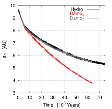
Figure 9: The evolution of the semi-major axis of the outer planet $a_{2}$, comparing a hydrodynamic model with two N-body calculations. The black curve (labeled Hydro) is the result of the full hydro model G. The lower dark gray curve is the damped N-body model using a constant damping $\tau=\tau_{0}$ in Eq. 6. The upper lighter gray curve (on top of the black one) is for time-dependent damping with a non-zero value of $\beta=1.0$, resulting in a much better match with the hydro model.

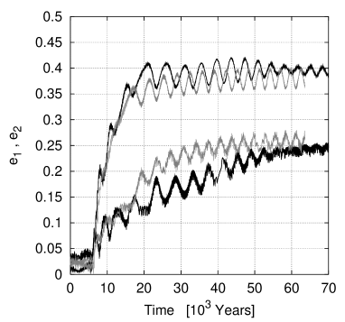
Figure 10: The evolution of the eccentricities of the inner planet (upper curves) and the outer planet (lower curves) for the full hydro model G (black curves covering the whole time range) and the damped N-body model (light gray), using a damping constant of $K=2.5$.

All the results of the damped N-body models are summarized in Tab. 3. The values of the damping constant $K$ cannot be determined too precisely, as there is some dependence of the magnitude on the initial eccentricities. Those were chosen to be about $0.01$ to $0.02$ for all models.

As an example, we display the evolution of model G, in which $H/r=0.05$. To test the damping, we first use Eq. (6) with a constant damping $\tau=\tau_{0}$, i.e. $\beta=0$. This refers to the lower (dark gray) curve in Fig. (9), where we chose $\tau_{0}=33,500$ yrs. As can be seen in the figure, a constant damping, even when it has the correct initial slope, in the longterm yields too fast a migration of the outer planet. A time-dependent damping with $\beta=1.0$ (light gray curve), leads to a much better fit with the hydrodynamic results. Additionally, we tested our method on published results for migrating single planets (Nelson et al. 2000), and find good agreement for suitable $\tau_{0}$ and $\beta$. Pure exponential fits for $a_{2}(t)$ with $\beta=0$ generally do not give satisfactory results.

This decrease in the damping rate as a function of time is a result of the reduction of mass in the disk, mainly due to the accretion of matter onto the outer planet. The mass flow across the gap is small, and the accretion rate onto the inner planet is substantially lower (see Kley 2000). However, if no gas is allowed to accrete onto the outer planet, a more substantial amount of gas may flow occur across the gap, leading to a smaller migration rate, or even outward migration (Masset & Snellgrove 2001; Masset 2002; Masset & Papaloizou 2003), because the angular momentum lost by the gap crossing material will be gained by the planet.

Besides $a$, we also compared the evolution of the eccentricity $e$ between the two approaches. In Fig. (10) we display the eccentricity evolution of the full hydro and the damped 3-body case for model G. Despite some differences which we attribute to the unknown eccentricity damping mechanism, the overall agreement is reasonable. For a given semi-major axis damping rate, the final values obtained for $e_{1}$ and $e_{2}$ at larger times depend on the initial values for the eccentricities and the amount of eccentricity damping. In this case we used an initial $e(t_{0})=0.01$ for both planets and an eccentricity damping factor $K=2.5$, i.e. a slightly shorter damping time scale for eccentricity as for semi-major axis. For all models we find that the eccentricity damping rate is of the same order as the semi-major axis damping, i.e. $K={\cal{O}}(1)$. This finding is in contrast to Lee & Peale (2002a) who determined a much shorter eccentricity damping time, based on models for GJ 876.

There are several possible reasons for this difference. Since the eccentricity damping of a planet is caused by material in the co-orbital region close to the planet, the treatment of this region in the models may have some effect on the results. In particular, the mass accretion onto the planet, the smoothing of the gravitational potential, and the numerical resolution may each play a significant role here. However, the simulations by Lee & Peale (2002a) are not based on clear physical model of the damping, but rather use an ad hoc prescription. Fitting to the observed case of GJ 876 yields a high value of $K$. On the other hand, it will be difficult to model the system HD 82943 with $K=100$ because of the high observed eccentricities.

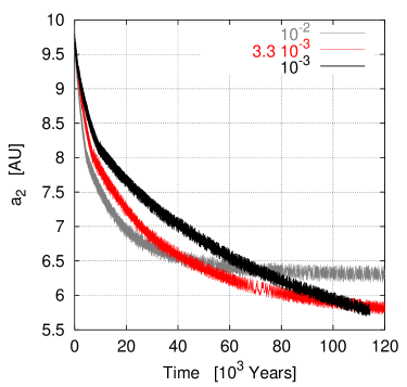
Figure 11: The time evolution of the outer planet’s semi-major axis for three models (C-E) with different viscosities. The corresponding $\alpha$ values are given in the legend

4.3 Dependence on the Physical Parameters

After describing the major effects of resonant capture and evolution we focus now on the dependence on the physical parameters. An overview of the results for all models is given in Tab. 4.

Table 4: Results of the full hydrodynamical computations for the longterm evolution. Listed are the model name, the resonance in which the system is captured, the eccentricity ratio $e_{2}/e_{1}$, the separation of the periastrae $\Delta{\varpi}$, the resonant angle $\Theta_{1}$, and the speed of the apsidal precession $\dot{{\varpi}}$. The models labeled with (V) are still evolving with time. For model D two cases (caught in different resonances) are presented.

Model	Res.	$e_{2}/e_{1}$	$\Delta{\varpi}$	$\Theta_{1}$	$\dot{{\varpi}}$
			[deg]	[deg]	[rad/yr]
A	3:1	1.0	-110	-140	- 0.0015
B	3:1	0.7	-120	-150	- 0.0015
C	3:1	0.73	-107	-145	- 0.0014
D1	2:1	0.35	0	0	- 0.0033
D2	3:1	0.70	+110	147	- 0.0015 (V)
E	3:1	0.73	-107	-140	- 0.0010
F	5:2	1.1	+180	0	- 0.0033
G	3:1	0.65	+110	+150	- 0.0022 (V)
X	2:1	0.24	0	0	- 0.0021

4.3.1 Viscosity

As the disk viscosity, parameterized here through the standard $\alpha$-parameter, determines the overall evolution of the disk, it is to be expected that its magnitude influences the longterm evolution of the planetary system as well. Starting from the standard model C ($\alpha=10^{-2}$) we performed additional runs using different values for the viscosity parameter $\alpha$; model D has $\alpha=3.3\cdot 10^{-3}$ and model E has $\alpha=10^{-3}$. The semi-major axis evolution for these models is shown in Fig. 11. For a single planet, the migration rate depends on the value of the viscosity (Nelson et al. 2000). Hence, the initial migration rates (during the first 10,000 yrs) are reduced for smaller $\nu$. The initial migration speeds for each model, as seen in Fig. 11, are quantified as $\tau_{0}$ in Tab. 3.

Upon capture of the inner planet, the migration rate of the outer slows down. Contrary to the expectation that smaller viscosities yield slower migration, we find that for these resonantly driven double-planet systems, the speed of migration is eventually faster for smaller viscosity coefficients. When the viscosity is lower, the migration slows down less rapidly (this would correspond to a lower $\beta$-value in the N-body method). This time-dependence of the damping is linked to the assumed mass accretion onto the planet. The accretion, which is larger for higher viscosity, lowers the mass of the disk with time and reduces the effective torques, such that migration drops off more rapidly for higher viscosity. The ratio of semi-major axis damping to eccentricity damping ($K$), however, does not appear to depend on the value of the viscosity. In all three cases we find capture into the 3:1 resonance (see Tab. 4), although this result is somewhat indeterminate. For the value of $\alpha=3.3\cdot 10^{-3}$, we also find a case in 2:1.

4.3.2 Temperature

Similarly to the viscosity, it may be expected that the scale height (temperature) of the disk will also influence the migration process of planets. Results for single planets (Kley 1999) have shown that for larger $H/r$ the gap is less cleared because the larger pressure gradient ‘pushes’ material into the gap. The higher density near the gap edges leads to a faster migration speed. This effect is indeed clearly seen in the early evolution of the planetary systems C & G, where the decline in the semi-major axis of the outer planet $a_{2}$ is faster for higher temperatures (see Fig. 12).

Upon capture however, the evolution behaves similarly to the case of varying viscosity. Those systems with higher $H/r$ now have the lowest migration speed. Similarly to the models with lower viscosity, smaller $H/r$ leads to lower accretion, higher disk mass, and hence more material pushing on the planets. As the migration slows down less for lower $H/r$, the overall evolution time scale becomes so long that it takes much more than $10^{5}$ yrs for the system to reach an equilibrium state. The intermediate model with $H/R=0.075$ is not displayed as is went into a 5:2 resonance.

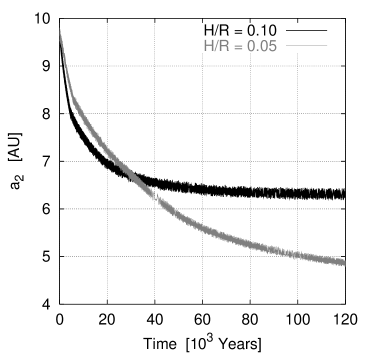
Figure 12: The evolution of the semi-major axis of the outer planet $a_{2}$ for two models (C, G) with different vertical disk scale heights, as indicated in the legend.

Figure 13: Results of a sequence of damped N-body simulations. Plotted is the difference of the periastrae $\Delta{\varpi}={\varpi}_{2}-{\varpi}_{1}$ of the two planets after capture into resonance versus planet mass, where $m_{p}=m_{2}=m_{1}$. The diamonds indicate capture in 2:1 resonance, while the plus signs are for 3:1 resonance. The other parameters are fixed, as described in the tex. The horizontal lines indicate values of $0$, $\pm 100^{o}$ and $\pm 180^{o}$.

4.3.3 Capture Probabilities

The main results of the full hydrodynamic calculations, as summarized in Tab. 4, show that for the same physical setup, capture in different resonances may occur. As a three body system is intrinsically chaotic, this indeterminate behavior may be expected.

Nevertheless, by running a whole sequence of fast damped N-body models, we can investigate what conditions determine the principle final outcome. The standard setup consists of two planets of $1M_{Jup}$ each, placed initially at 4 and 12 AU from the central $1M_{\odot}$ star. The initial eccentricities are $0.02$. As in all previous models, only the orbit of the outer planet is damped, using in these cases a damping time scale $\tau_{0}=20,000$ yrs. We fix the damping constants to $\beta=1.0$ and $K=1.0$. Starting from this standard case, we vary the damping time scale $\tau_{0}$, the initial eccentricity $e_{2}$, and mass of the outer planet $m_{2}$, while keeping always identical planet masses, $m_{1}=m_{2}$.

In the standard case, the planets are caught in a 2:1 resonance. Varying the time scale $\tau_{0}$ from 10,000 to 50,000 yrs, there is no capture into higher resonances. Upon variation of eccentricity $e_{2}$ from 0.0 to 0.5, we find that for $e_{2}<0.25$ capture occurs always into 2:1, while for larger $e_{2}$ higher order resonances (primarily 3:1) are possible, however with no definite outcome. The influence of the planet mass is illustrated in Fig. 13, where the resonance type (2:1 diamonds, 3:1 plus signs) is shown as a function of planet mass (with $m_{1}=m_{2}$). For small planets with $m_{p}<1.7M_{Jup}$, capture occurs robustly into the 2:1 resonance. Higher resonances are possible only for $m_{p}$ larger than this value. However, due to the chaotic nature of the problem the exact outcome for a particular $m_{p}$ is not predictable. This is in agreement with the hydrodynamic simulations where we also find capture in different resonances just by perturbing the initial density slightly (compare models D1, D2).

4.3.4 The Resonant Angles

In the majority of hydrodynamic models, the planets catch each other in a 3:1 resonance. As demonstrated above, this is mainly a consequence of the large masses chosen for the planets. For all models the resonant angles settle to $|\Delta{\varpi}|\approx 110^{o}$ and $|\Theta_{1}|\approx 145^{o}$, with some scatter of about $\pm 10^{o}$. For the damped N-body models we checked the values of the resonant angles as well, finding that all 2:1 resonances settle into the complete symmetric configuration $\Delta{\varpi}=\Theta_{1}=0$ (Fig. 13). For the 3:1 resonances we see anti-symmetric configurations with anti-aligned periastrae, $|\Delta{\varpi}|=180^{0}$ and $\Theta_{1}=0$ for masses around $m_{p}=2M_{Jup}$, (when the first 3:1 cases begin to occur), while for all larger masses we find preferentially the previous non-symmetric configurations. This behavior is again an indication of a bifurcation in the stability properties of resonant systems, as claimed by Beauge et al. (2002). With additional damped N-body calculations we also find that systems entering a 5:2 resonance (not shown) exhibit a typical anti-symmetric behavior $|\Delta{\varpi}|=180^{0}$ and $\Theta_{1}=0^{o}$.

5 Summary and Conclusion

We have performed full hydrodynamical calculations simulating the joint evolution of a pair of protoplanets together with the surrounding protoplanetary disk from which they originally formed. The focus lies on massive planets in the range of a few Jupiter masses. For the disk evolution we solve the Navier-Stokes equations, and the motion of the planets is followed using a 4th order Runge-Kutta scheme, which includes their mutual interactions as well as the star and disk’s gravitational fields. These results were compared to simplified (damped) N-body computations, where the gravitational influence of the disk is modeled through analytic damping terms applied to the semi-major axis and eccentricity.

We find that both methods yield comparable results, if the damping constants in the simplified models are adjusted properly. The mass reduction of the disk with time, due for example to mass accretion onto the planet, or possible mass flow across the outer planet’s gap can be modeled satisfactorily through a damping time scale, which depends linearly on time. The eccentricity damping was always chosen to be a constant multiple $K$ of the semi-major axis damping. In this case we find that $K$ must be of order unity to match the hydrodynamic models.

However, fitting N-body models to the observed parameters of GJ 876 requires a high $e$-damping with typically $K=100$ (see also Lee & Peale 2002a), relatively independent of the functional behavior of $a_{2}(t)$. Reasons for this discrepancy may lie in the simplified hydrodynamical model, which uses a fixed equation of state, a simple treatment of the planetary structure, and only an approximate model of the torques acting on the planet. Also, eccentricity damping is dominated by material close to the planet; the insufficient numerical grid resolution near the planet may smear out the damping forces. In addition, the accretion process of matter onto the planet is reducing the mass in the co-orbital region which lowers the eccentricity damping. The simplified assumption of a constant value of $K$ needs to be checked. More detailed hydrodynamical models may help to resolve this discrepancy in the future. An alternative explanation for the low eccentricities in GJ 876 compared to our hydrodynamic simulations is that further evolution of the eccentricities occurs in the system after planet and gap formation. The planet eccentricities may be further modified as the disk dissipates and its resulting eccentricity forcing gradually declines. On the other hand, the assumption of a constant value of $K$ in the N-body models in the computations by Lee & Peale (2002a) is also not based on any detailed hydrodynamic model but rather assumed ab initio. In more general models, this will have to be relaxed.

The case HD 82943 is also not easy to model as the eccentricities for both planets are very large, which turned out to be very difficult to capture with N-body models, even with very low damping. The problem here lies in the stability of the resulting system. All test computations with constant values of $K$ eventually led to unstable systems. Compared to GJ 876, the eccentricity damping for HD 82943 must be orders of magnitude less, if otherwise similar physical parameters are used. In order to explain the high eccentricities, the inclusion of an additional companion may be necessary.

Despite of the difficulty of the models to obtain the observed eccentricities, there are nevertheless several features of the observed 2:1 planets which are captured correctly by our simulations: i) The larger mass of the outer planet, ii) the higher eccentricity of the inner planet, and iii) the periastrae separation of $\Delta{\varpi}=0^{o}$. These are robust predictions of the hydrodynamic models.

For 3:1 resonances, anti-symmetric ($\Delta{\varpi}=180^{o}$) and non-symmetric final configurations are obtained. In the non-symmetric case we found over a range of models a value of $|\Delta{\varpi}\approx 110^{o}|$, which is supported by stability analysis (Beauge et al. 2002). In 55 Cnc, the only observed 3:1 case, there are other planets present in the system, which makes an interpretation using just this simple treatment questionable.