O stars effective temperature and H II regions ionization parameter
gradients in the Galaxy

Abstract

Extensive photoionization model grids are computed for single star H II regions using stellar atmosphere models from the WM-Basic code. Mid-IR emission line intensities are predicted and diagnostic diagrams of [Ne III/ II] and [S IV/ III] excitation ratio are build, taking into account the metallicities of both the star and the H II region. The diagrams are used in conjunction with galactic H II region observations obtained with the ISO Observatory to determine the effective temperature $T_{\rm{eff}}$ of the exciting O stars and the mean ionization parameter $\bar{U}$. $T_{\rm{eff}}$ and $\bar{U}$ are found to increase and decrease, respectively, with the metallicity of the H II region represented by the Ne/Ne_⊙ ratio. No evidence is found for gradients of $T_{\rm{eff}}$ or $\bar{U}$ with galactocentric distance R_gal. The observed excitation sequence with R_gal is mainly due to the effect of the metallicity gradient on the spectral ionizing shape, upon which the effect of an increase in $T_{\rm{eff}}$ with $Z$ is superimposed. We show that not taking properly into account the effect of metallicity on the ionizing shape of the stellar atmosphere would lead to an apparent decrease of $T_{\rm{eff}}$ with $Z$ and an increase of $T_{\rm{eff}}$ with R_gal.

1. Introduction

The determination of the stellar distribution (especially of the hottest stars) and physical characteristics of galactic H II regions are of primary importance to evaluate star formation theories and for our understanding of the chemical evolution of galaxies.

Shields & Tinsley (1976) used the equivalent width of the H_β emission from H II regions in spiral galaxies to determine the existence of a radial gradient in the effective temperature (hereafter $T_{\rm{eff}}$) of the hottest stars, associated with a decrease in metal abundance. Campbell (1988) determined $T_{\rm{eff}}$ and the ionization parameter $U$ for various H II galaxies, and concluded that the $T_{\rm{eff}}$ of the hottest star decreases with increasing oxygen abundance.

On the other hand, Evans & Dopita (1985) have computed extensive photoionization models, using Hummer & Mihalas (1970) atmosphere models, and have determined from optical observations of H II regions that the ionization temperature of the exciting stars is approximately constant (41 kK, independently of the metallicity $Z$ and $U$). They found, however, an anticorrelation between $U$ and $Z$. Fierro et al. (1986) found a near constant $T_{\rm{eff}}$ of 35 kK between 1 and 5 kpc from the center of NGC 2403.

More recently, Martín-Hernández et al. (2002b) used Infrared Space Observatory (ISO) spectral observations of galactic H II regions to show that the gas excitation increases with the galactocentric distance R_gal. They concluded that the stellar spectral energy distributions (hereafter SEDs) are softer at higher metallicities, that is towards the galactic center and that the SED changes can explain the observed gradient. Giveon et al. (2002b) similarly used ISO observations, but suggest that the increase in excitation correspond instead to a decrease in stellar effective temperature. Morisset et al. (2003, hereafter MSBM03) show that excitation gradients are partly due to changes in the ionizing spectral shape of O stars with metallicity. They concluded that the excitation scatter is probably mainly due to randomization of both the stellar $T_{\rm{eff}}$ and the nebular mean ionization parameter $\bar{U}$.

No attempt was made by Giveon et al. (2002b), Martín-Hernández et al. (2002b), nor in MSBM03 to determine $T_{\rm{eff}}$ and $U$ for individual H II regions.

Dors & Copetti (2003) used optical observations of galactic and magellanic H II regions to determine $T_{\rm{eff}}$ from optical diagnostic line ratios. They also found an increase of $T_{\rm{eff}}$ with the galactocentric distance.

The aim of the present work firstly is to build diagnostics diagrams for the determination of $T_{\rm{eff}}$ and $\bar{U}$, based on mid-IR emission lines. The diagrams are derived from a extensive grid of photoionization models that populate the $T_{\rm{eff}}$-$\bar{U}$-$Z$ space and use the WM-Basic (Pauldrach et al., 2001) code to compute the ionizing atmosphere models. In a second step, $T_{\rm{eff}}$ and $\bar{U}$ are determined for the ISO H II regions using the new diagnostic diagrams.

Sect. 2 describes the ISO observations of H II regions, and Sect. 3 the grid of photoionization models. The location of ISO observations in the model grids, and the process to determine $T_{\rm{eff}}$, and the mean ionization parameter $\bar{U}$ for every object are presented in Sect. 4, using two different methods. Sect. 5 describes the resulting gradients of $T_{\rm{eff}}$ and $\bar{U}$. The effect of the stellar metallicity in the determination of $T_{\rm{eff}}$ is discussed in Sect. 6, in particular the influence of the changes in the stellar SEDs with metallicity. The conclusions are presented in Sect. 7.

2. ISO Observations of H II regions

Mid-IR fine-structure line intensities obtained from observations of H II regions with ISO-SWS (Martín-Hernández et al., 2002a; Giveon et al., 2002b) are used here to determine the various stellar and nebular parameters.

Line ratios of [Ar III]8.98$\mu$m / [Ar II]6.98$\mu$m, [S IV]10.5$\mu$m / [S III]18.7$\mu$m, and [Ne III]15.5$\mu$m / [Ne II]12.8$\mu$m (hereafter [Ar III/ II], [S IV/ III] and [Ne III/ II] resp.) are then used to build excitation diagrams (see MSBM03 for more details). The line intensities were corrected for reddening by Giveon et al. (2002a). Once the sources for which at least one of the line intensities used in this work is not defined (or have only an upper limit) are removed, 42 usable sources remain.

3. Grid of photoionization models

A grid of photoionization models using the NEBU code (Morisset et al., 2002) has been calculated using ionizing spectral distributions from supergiant atmosphere models that were computed with WM-Basic V. 2.11 (Pauldrach et al., 2001). The current grid of photoionisation models is similar to the one used in MSBM03 (see MSBM03 for details). It has been extended further to encompass the full range of values expected within the 3D parameters space $T_{\rm{eff}}$-$\bar{U}$-$Z$. $T_{\rm{eff}}$ is ranging from 30 to 50 kK, by 5 kK steps, $\log(\bar{U})$ being -2.6, -1.5, -0.8, -0.1 and 0.5, and the metallicity $Z$ of both the ionizing star and the nebular gas being 0.5, 0.75, 1.0, 1.5 and 2.0 times the solar value (as defined in WM-Basic). In total, 125 models have been computed from which mid-IR line intensities were derived.

4. Determination of $T_{\rm{eff}}$ and $\bar{U}$

Three mid-IR line ratios could in principle be used as excitation diagnostics, namely [Ar III/ II], [Ne III/ II] and [S IV/ III]). We note however that [Ar III/ II] is overestimated in photoionization models, as pointed out in MSBM03. It is not clear whether the latter is due to an improper determination of the ionizing flux near 24 eV or simply to incomplete atomic physics used within photoionization codes (e.g. missing accurate dielectronic recombination rates). For these reasons, despite its low dependence on $\bar{U}$, the [Ar III/ II] ratio proves to be useless for determining $T_{\rm{eff}}$. On the other hand, while the alternative excitation ratios [Ne III/ II] and [S IV/ III] are both sensitive to $T_{\rm{eff}}$ and $\bar{U}$, it turns out that the effect of either parameter on both ratios is somewhat different, and a way to determine $T_{\rm{eff}}$ and $\bar{U}$ using these excitation diagnostics can be extracted. Even though the direct use of [Ne III/ II] and [S IV/ III] or other combinations of these line ratios would provide equivalent constraints; we prefer to adopt $\eta_{\rm S-Ne}$, defined following Vilchez & Pagel (1988) as $\eta_{\rm S-Ne}$ = [S IV/ III] / [Ne III/ II], in combination with [Ne III/ II]. The determination of $T_{\rm{eff}}$ and $\bar{U}$ turns out to be clearer and easier to read off when using $\eta_{\rm S-Ne}$.

The underlying hypothesis/assumptions made here are the following: 1) the ISO H II regions are excited by a single star (i.e. the presence of other less luminous stars doesn’t affect the results), 2) the H II regions are ionized by stars of comparable surface gravity $\log(g)$ at a given $T_{\rm{eff}}$ (see MSBM03 for the effects of $\log(g)$), 3) the Ne abundance determined from an H II region is a reliable estimator of the ionizing star metallicity, 4) the presence of dust in the H II regions doesn’t affect the $T_{\rm{eff}}$ and $\bar{U}$ gradients. Dust would decrease the global amount of ionizing photons, but also increase the hardness of the ionizing SED, increasing the excitation of the gas depicted by the IR excitation diagnostics (see MSBM03) and therefore the $T_{\rm{eff}}$ we infer can be overestimated, 5) Using a nebular geometry consisting of a simple shell does not affect the diagnostic diagrams, 6) the WM-Basic atmosphere models describe well the ionizing flux between 35 and 41 eV (or at least the relative changes that occurs when the parameters $T_{\rm{eff}}$ or $Z$ are varied).

4.1. S-Method : Using only solar metallicity atmosphere models

In a first step, we use only the results of the photoionization models obtained with the solar abundances atmosphere models.

The Fig. 1 shows the values taken by $\eta_{\rm S-Ne}$ and [Ne III/ II], when $T_{\rm{eff}}$ and $\bar{U}$ are varied in locked steps. For each H II region, 2D-interpolations within this grid are performed and used to determine $T_{\rm{eff}}$ and $\bar{U}$. All the observed values lie inside the grids, no extrapolation is needed. The $T_{\rm{eff}}$ and $\bar{U}$ obtained with solar metallicity atmosphere models are presented in Sec. 5.

From Fig. 1, we can determine the effects of uncertainties in line intensities on $T_{\rm{eff}}$ and$\bar{U}$: a factor of two in the excitation diagnostics leads to a shift in $T_{\rm{eff}}$ by 1 kK and in $\bar{U}$ by 0.5 dex.

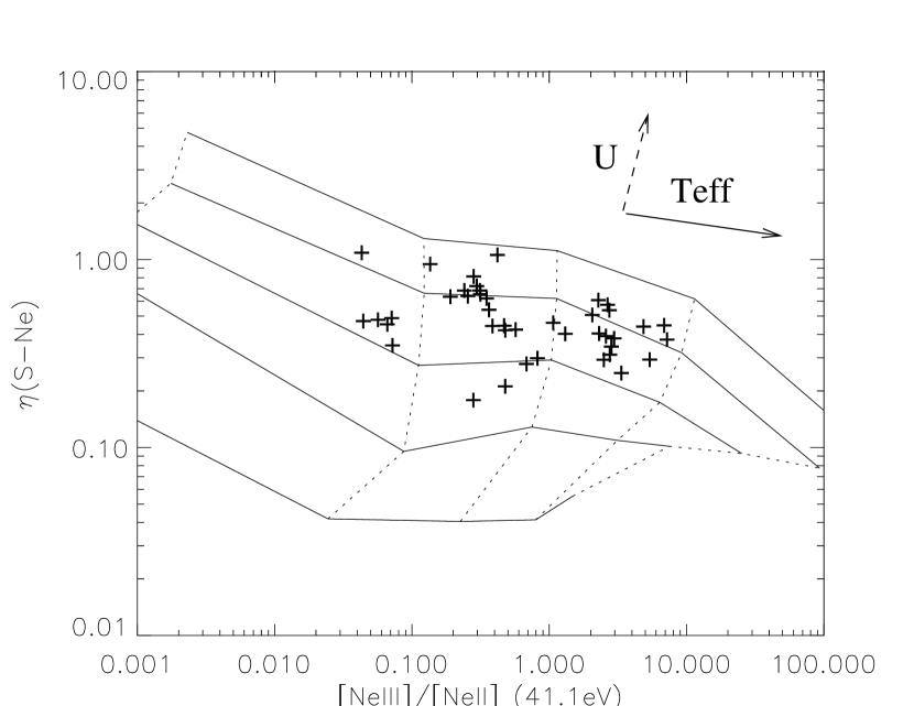
Figure 1.— The $\eta_{\rm S-Ne}$ versus [Ne III/ II] excitation diagram for the H II regions observed by ISO. The grid of photoionization model with stellar and nebular metallicity given by $Z/Z_{\odot}$ = 1.0 (S-Method) is drawn. Solid (dotted) lines connect iso-$\bar{U}$ (iso-$T_{\rm{eff}}$) models. $T_{\rm{eff}}$ and $\log(\bar{U})$ take values of 30, 35, 40, 45, 50 kK and -2.6, -1.5, -0.8, -0.1, 0.5, respectively.

4.2. Z-Method : $T_{\rm{eff}}$ and $\bar{U}$ obtained using Z-dependent atmosphere models

The chemical composition of a star strongly affects its radiation, especially in the EUV, where the ionizing photons are emitted. For the same $T_{\rm{eff}}$, changing the stellar luminosity by a factor of 4 can affect the excitation diagnostic line ratios by up to 2 orders of magnitude (MSBM03). The determination of $T_{\rm{eff}}$ and $\bar{U}$ need then to be performed using grids of photoionization models with various stellar metallicities, as described in Sect. 3. Making the assumption that the metallicity of the ionized region reflects the metallicity of the ionizing star, we can use adapted diagnostic grids, corresponding to the H II regions metallicities, to determine $T_{\rm{eff}}$ and $\bar{U}$. The metallicity of an H II region is hereafter given by the abundance ratio Ne/Ne_⊙ = [Ne/H]/[Ne/H]_⊙, where [Ne/H] is obtained from Giveon et al. (2002a). The solar abundance used, [Ne/H]${}_{\odot}=1.4\times 10^{-4}$, is defined as the value of the abundance gradient [Ne/H](R_gal) found by Giveon et al. (2002a), evaluated at 8.5 kpc. The Ne abundances as a measure of $Z/Z_{\odot}$, are preferred to a combination of Ne, Ar and S abundances, since, for these two last elements, the abundances are not reliable when the excitation is extreme (MSBM03). For each H II region, we extract from the $T_{\rm{eff}}$-$\bar{U}$-$Z$ photoionization model grid the $T_{\rm{eff}}$-$\bar{U}$ plane, whose metallicity lies closest to the Ne/Ne_⊙ of the H II region. The Fig. 2 shows, for the 5 metallicities used in the photoionization model grid, the values taken by $\eta_{\rm S-Ne}$ and [Ne III/ II]. The effect of increasing the metallicity of the atmosphere models (and consequently of the nebular gas) is clearly to increase the value of $T_{\rm{eff}}$ for a given [Ne III/ II] ratio, as already pointed out in MSBM03. The observed values for the H II regions are also plotted in the diagramm corresponding to their metallicities. All the observed values lie inside the grids. 2D-Interpolations are performed to determine $T_{\rm{eff}}$ and $\bar{U}$ for each H II region.

Figure 2.— Same as Fig. 1 but the stellar and nebular metallicities beeing 0.5, 0.75, 1.0, 1.5, 2.0 times solar, from upper left to lower right. Solid (dotted) lines connect iso-$\bar{U}$ (iso-$T_{\rm{eff}}$) models. $T_{\rm{eff}}$ and $\log(\bar{U})$ take values of 30, 35, 40, 45, 50 kK and -2.6, -1.5, -0.8, -0.1, 0.5, respectively. All the observations of the H II regions are distributed in the diagramms, according to their nearest values of Ne/Ne_⊙ (Z-Method). The H II regions are symbolized using X, W, +, 0, and = for Ne/Ne_⊙ = 0.5, 0.75, 1.0, 1.5, 2.0, respecively. See Tab. 1 for the correspondance between sources and the diagramm used.

5. Results

The Table 1 presents the characteristics of the 42 H II regions used in this work: R_gal, Ne/Ne_⊙ (with a symbol corresponding to the grid used within the Z-Method, Sec. 4.2), [Ne III/ II], [S IV/ III], and the $T_{\rm{eff}}$ and $\bar{U}$ obtained using the Z-Method. The $T_{\rm{eff}}$ range from 34 to 50 kK, and $\log(\bar{U})$ from -1.5 to 0.5, with mean values of 40.5 kK and -0.60, respectively. Such range for $T_{\rm{eff}}$ and $\bar{U}$ is in agreement with the results found by Evans & Dopita (1985). For the 3 sources for which two independent observations are available, the results obtained lead to a coherent determination of $T_{\rm{eff}}$, while the values of $\bar{U}$ can differ by a factor up to 5.

The set of inferred values for $T_{\rm{eff}}$ and $\log(\bar{U})$ versus the galactocentric radius R_gal and the abundance ratio Ne/Ne_⊙ are shown in Fig. 4 for the S-Method (Sec. 4.1), and in Fig. 4 for the Z-Method (Sec. 4.2). Linear fit to the data are also presented in all the figures.

The results obtained for $T_{\rm{eff}}$ with S- and Z-Methods are very different (upper panels of Figs. 4-4). While S-Method leads to an increase (decrease) of $T_{\rm{eff}}$ with R_gal (Ne/Ne_⊙), the use of the Z-Method leads to rather different results: no clear correlation is found to exist between $T_{\rm{eff}}$ and R_gal while a correlation is present between $T_{\rm{eff}}$ and Ne/Ne_⊙. The distribution of $T_{\rm{eff}}$ versus Ne/Ne_⊙ obtained with the Z-Method can also be described as follows: $T_{\rm{eff}}$ increasing strongly with Ne/Ne_⊙ for Ne/Ne_⊙$<1.2$, and a quasi constant value ($\sim 43$ kK) for higher Ne/Ne_⊙, coupled with a higher dispersion.

The dispersion of Ne/Ne_⊙ with position in the Galaxy is relatively high (see the symbols dispersion along R_gal in the left panels of Fig. 4). The absence of correlation between $T_{\rm{eff}}$ and R_gal obtained with Z-Method might be the result of this high dispersion. Note that for H II regions with R_gal$<$R_gal⊙, the determination of R_gal is degenerate (Martín-Hernández et al., 2002a) and the errors are also important.

Virtually no changes are observed for $\log(\bar{U})$ from S- to Z-Method (lower panels of Figs. 4-4). This gives insights of the robustness of our results concerning $\bar{U}$ whatever the method used. This can be understood as follows: the main effect of changing $Z$ on the diagnostic diagrams (Fig. 2) is to shift horizontally ([Ne III/ II] axis) the grids of models, while the determination of $\bar{U}$ is mainly dependent on the vertical position along the $\eta_{\rm S-Ne}$ axis, which is not affected by the stellar metallicity. No clear correlation is found between $\bar{U}$ and R_gal but an inverse correlation between $\bar{U}$ and Ne/Ne_⊙ is present (see Fig. 4, lower panels).

Fig. 5 shows the distribution of $T_{\rm{eff}}$ versus the [Ne III/ II] excitation ratio. The softening of the stellar emission when the metallicity increases (even if $T_{\rm{eff}}$ doesn’t change) is enough to cover the whole observed range of [Ne III/ II] (over 2.5 dex). This Fig. 5 illustrates one more time the illusion of determining $T_{\rm{eff}}$ from only one excitation diagnostic.On the other hand, a global increase of $T_{\rm{eff}}$ with [Ne III/ II] is also present (the hottest stars are associated with the most excited H II regions).

Namea	Rgalb	Ne/Ne⊙c	[Ne III/ II]c	[S IV/ III]d	$T_{\rm{eff}}$e,f	$\bar{U}$f
GCRINGSW	0.00	2.221=	0.048	0.021	39.5	0.302
ARCHFILNW	0.00	2.340=	0.037	0.016	38.8	0.280
IRAS 17455-2800	0.50	1.645O	0.405	0.156	42.3	0.213
SGR D HII	1.50	1.410O	0.398	0.161	42.2	0.241
WBH9815567-5236	4.30	0.773W	0.355	0.343	35.5	2.521
RAFGL 2094	4.40	1.647O	0.056	0.023	36.1	0.297
IRAS 18317-0757	4.50	1.895=	0.060	0.027	40.1	0.314
WBH9818317-0757	4.50	2.139=	0.061	0.020	40.2	0.163
GAL 033.91+00.11	4.50	0.970+	0.482	0.187	38.2	0.282
IRAS 15502-5302	4.60	0.932+	0.216	0.126	36.3	0.630
IRAS 18434-0242	4.60	1.755=	0.251	0.165	45.2	0.508
IRAS 18502+0051	4.80	1.987=	0.204	0.127	44.5	0.437
GRS 328.30+00.43	4.80	0.741W	0.239	0.177	34.9	1.148
IRAS 17221-3619	5.20	1.706O	0.036	0.036	34.9	2.007
WBH9816172-5028	5.60	1.707O	0.327	0.132	41.5	0.244
GAL 337.9-00.5	5.80	2.076=	0.578	0.147	48.2	0.060
G327.3-0.5	6.30	1.912=	0.405	0.078	47.3	0.038
WBH9817059-4132	6.30	2.386=	0.237	0.039	45.5	0.034
GAL 045.45+00.06	6.30	1.450O	0.905	0.381	45.3	0.268
IRAS 15384-5348	6.40	1.384O	0.296	0.168	41.0	0.500
GRS 326.44+00.91	6.50	1.284O	0.308	0.152	41.2	0.372
WBH9815408-5356	6.60	1.768=	0.695	0.189	48.7	0.066
M17IRAMPOS8	6.80	1.363O	2.839	0.646	49.7	0.074
W51 IRS2	7.30	1.106+	1.743	0.807	41.1	0.596
NGC6357I	7.70	1.169+	1.107	0.407	40.1	0.270
S106 IRS4	8.40	0.742W	0.115	0.099	34.0	1.326
NGC3603	8.90	1.524O	2.513	0.873	48.3	0.240
IRAS 12063-6259	9.30	0.775W	1.930	1.071	38.4	1.242
GAL 289.88-00.79	9.30	0.765W	0.267	0.159	35.0	0.716
IRAS 10589-6034	9.50	0.853W	0.265	0.165	35.0	0.799
RAFGL 4127	9.60	0.827W	4.116	1.654	39.7	0.759
BE83IR 070.29+0	9.60	0.547X	1.954	0.721	34.4	0.377
BE83IR 070.29+0	9.60	0.414X	2.115	0.566	35.1	0.086
IRAS 11143-6113	9.70	1.037+	4.571	1.226	43.7	0.342
IRAS 19598+3324	9.80	0.432X	2.192	0.784	34.5	0.329
IRAS 12073-6233	10.10	0.733W	5.813	2.368	40.2	1.093
GAL 298.23-00.33	10.10	0.627W	6.110	2.091	40.4	0.803
IRAS 02219+6152	11.00	0.986+	2.402	0.755	42.1	0.317
IRAS 02219+6152	11.00	1.016+	2.252	1.182	41.6	0.887
W3 IRS2	11.30	0.961+	2.339	0.665	42.1	0.250
W3 IRS2	11.30	0.943+	2.321	1.139	41.7	0.820
S156 A	11.50	0.820W	0.161	0.094	34.4	0.607

Table 1 Sources parameters and corresponding $T_{\rm{eff}}$ and $\bar{U}$ determined in this paper. ^a: IRAS named sources from Martín-Hernández et al. (2002a), otherwise from Giveon et al. (2002b). ^b: R_gal in Kpc. ^c: Upper symbols indicat which grid is used to determine $T_{\rm{eff}}$ and $\bar{U}$: X, W, +, O, = correspond to the Ne/Ne_⊙ = 0.5, 0.75, 1.0, 1.5 and 2.0 grid resp. (See Fig. 2) ^d: Line intensities corrected for reddening, see text. ^e: $T_{\rm{eff}}$ in kK. ^f: Values obtained using the Z-Method (Sec. 4.2).

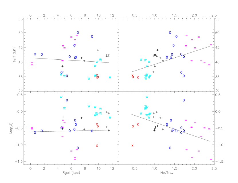
Figure 3.— $T_{\rm{eff}}$ (upper panels) and $\bar{U}$ (lower panels) versus R_gal (left) and Ne/Ne_⊙ (right) for the sample of H II regions. The grid of photoionization models results computed with $Z=Z_{\odot}$ stars show in Fig. 1 is used for every source (S-Method, Sec. 4.1). Linear fits to the data are presented.

Figure 4.— Same as in Fig. 4, but each H II region is symbolized according to its abundance Ne/Ne_⊙ as in Fig. 2. The determination of $T_{\rm{eff}}$ and $\bar{U}$ follows from the use of the appropriate diagnostic diagram from Fig. 2 (Z-Method, Sec. 4.2). Linear fits to the data are presented.

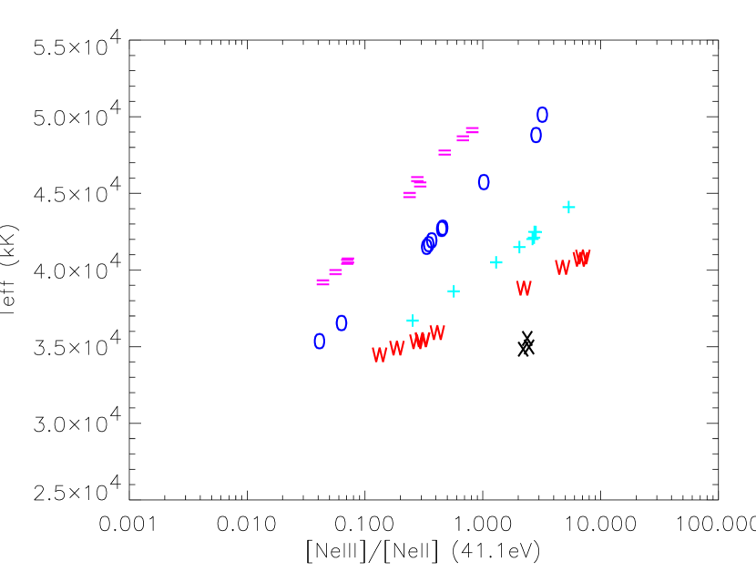
Figure 5.— $T_{\rm{eff}}$ versus [Ne III/ II] for the ISO H II regions. Symbols as in Fig.4.

6. Discussion

The results presented in Sect. 5 are sensitive to the changes of the stellar SED with metallicity, for a given atmosphere model code. The gradients in $T_{\rm{eff}}$ as a function of Ne/Ne_⊙ and R_gal derived from a single solar metallicity set of stars (S-Method) are very different from the gradients obtained with coherent metallicity for the stellar atmosphere model (Z-Method).

The results obtained with the S-Method agree with those of Campbell (1988) and Dors & Copetti (2003), who similarly didn’t take into account the $Z$-dependence of the stellar emission. This confirms that the trends seen in the upper panels of Fig. 4, when the $Z$-dependence is properly considered, are mainly due to the changes in the stellar SEDs when the metallicity decreases (an effect which has to be present, but whose magnitude might depend on the family of atmosphere models used). Dors & Copetti (2003) check the effect of metallicity on the excitation of the ionized gas, but didn’t found a strong effect; the metallicity range they test is only a factor of two for WM-Basic models, they used a low value for the ionization parameter, the effect of $Z$ being reduced in this case, and they used dwarf WM-Basic models, for which the effect of $Z$ is lower than for supergiants. The $T_{\rm{eff}}$ values obtained by Campbell (1988) and Dors & Copetti (2003) are derived using a S-Method, and the apparent decrease of $T_{\rm{eff}}$ with $Z$ and increase of $T_{\rm{eff}}$ with R_gal that they respectively found is likely to be the result of not considering $Z$-dependent stellar models (the excitation of the gas is not a valid $T_{\rm{eff}}$ indicator, as shown by Fig. 5). Note also that the maximum $T_{\rm{eff}}$ obtained with S-Method is 45 kK, while the $T_{\rm{eff}}$ values from Z-Method get as high as 50 kK.

The results shown in this paper concerning $T_{\rm{eff}}$ and $\bar{U}$ are strongly dependent on the kind of atmosphere model used to compute the photoionization grid of models. In MSBM03, we discuss in detail the major differences between, for instance, WM-Basic and CMFGEN (Hillier & Miller, 1998), in sofar as the determination of $T_{\rm{eff}}$ is concerned. Using the CMFGEN instead of WM-Basic atmosphere models would certainly lead to a globally lower $T_{\rm{eff}}$ (MSBM03), and perhaps different gradients.

The increase of $T_{\rm{eff}}$ with $Z$ found here is in contradiction with the theoretical predictions of e.g. Schaller et al. (1992), and if confirmed it might have profond implications for the study of the upper mass end of the IMF.

However, more extensive studies will be needed to check whether the use of different atmospheres codes will confirm the gradients found here or generate genuine gradients. Our results, nevertheless, show the importance of taking properly into account the variation in the stellar SEDs with metallicity in any attempt to determine a reliable $T_{\rm{eff}}$ from H II regions.

7. Summary and Conclusion

Based on WM-Basic atmosphere models we have computed a large set of photoionisation models. From these models we have built excitation diagnostic diagrams based on [Ne III/ II] and [S IV/ III] (mid-IR lines) excitation ratios. ISO observations of galactic H II regions are superimposed to these diagrams. According to their metallicity, $T_{\rm{eff}}$ and $\bar{U}$ are determined for every H II region.

A correlation between $T_{\rm{eff}}$ and Ne/Ne_⊙, and an anti-correlation between $\bar{U}$ and Ne/Ne_⊙, have been found, without evidence of any correlation between both $T_{\rm{eff}}$ and $\bar{U}$ versus R_gal. The determination of $T_{\rm{eff}}$ is strongly dependent on the changes in stellar SEDs due to the radial metallicity gradient within the Galaxy, while the results found concerning the behaviour of $\bar{U}$ are globally insensitive to this effect. The gaseous excitation sequence is therefore mainly driven by the effects of metallicity on the stellar SEDs. A global increase of $T_{\rm{eff}}$ with metallicity appears nevertheless to be present. More investigation using different atmosphere codes will be needed to confirm that our conclusions are not unduly biased toward the use of WM-Basic models. Comparison with $T_{\rm{eff}}$ determined from direct observations of ionizing stars can also help to evaluate the robustness of the method presented in this work.

References

- Campbell (1988) Campbell, A. 1988, ApJ, 335, 644
- Dors & Copetti (2003) Dors, O. L. & Copetti, M. V. F. 2003, A&A, 404, 969
- Evans & Dopita (1985) Evans, I. N. & Dopita, M. A. 1985, ApJS, 58, 125
- Fierro et al. (1986) Fierro, J., Torres-Peimbert, S., & Peimbert, M. 1986, PASP, 98, 1032
- Giveon et al. (2002a) Giveon, U., Morisset, C., & Sternberg, A. 2002a, A&A, 392, 501
- Giveon et al. (2002b) Giveon, U., Sternberg, A., Lutz, D., Feuchtgruber, H., & Pauldrach, A. W. A. 2002b, ApJ, 566, 880
- Hillier & Miller (1998) Hillier, D. J. & Miller, D. L. 1998, ApJ, 496, 407
- Hummer & Mihalas (1970) Hummer, D. G. & Mihalas, D. 1970, MNRAS, 147, 339
- Martín-Hernández et al. (2002a) Martín-Hernández, N., Peeters, E., E. Damour, F., Cox, P., Roelfsema, P., Baluteau, J.-P., Tielens, A., Churchwell, E., Jones, A., Kessler, M., Mathis, J., Morisset, C., & Schaerer, D. 2002a, A&A, 381, 606
- Martín-Hernández et al. (2002b) Martín-Hernández, N. L., Vermeij, R., Tielens, A. G. G. M., van der Hulst, J. M., & Peeters, E. 2002b, A&A, 389, 286
- Morisset et al. (2003) Morisset, C., Schaerer, D., Bouret, J.-C., & Martins, F. 2003, A&A, (MSBM03) accepted, see astro-ph/0310151
- Morisset et al. (2002) Morisset, C., Schaerer, D., Martín-Hernández, N. L., Peeters, E., Damour, F., Baluteau, J.-P., Cox, P., & Roelfsema, P. 2002, A&A, 386, 558
- Pauldrach et al. (2001) Pauldrach, A. W. A., Hoffmann, T. L., & Lennon, M. 2001, A&A, 375, 161
- Schaller et al. (1992) Schaller, G., Schaerer, D., Meynet, G., & Maeder, A. 1992, A&AS, 96, 269
- Shields & Tinsley (1976) Shields, G. A. & Tinsley, B. M. 1976, ApJ, 203, 66
- Vilchez & Pagel (1988) Vilchez, J. M. & Pagel, B. E. J. 1988, MNRAS, 231, 257