Phase Correlations in Cosmic Microwave Background Temperature Maps

Abstract

We study the statistical properties of spherical harmonic modes of temperature maps of the cosmic microwave background. Unlike other studies, which focus mainly on properties of the amplitudes of these modes, we look instead at their phases. In particular, we present a simple measure of phase correlation that can be diagnostic of departures from the standard assumption that primordial density fluctuations constitute a statistically homogeneous and isotropic Gaussian random field, which should possess phases that are uniformly random on the unit circle. The method we discuss checks for the uniformity of the distribution of phase angles using a non-parametric descriptor based on the use order statistics, which is known as Kuiper’s statistic. The particular advantage of the method we present is that, when coupled to the judicious use of Monte Carlo simulations, it can deliver very interesting results from small data samples. In particular, it is useful for studying the properties of spherical harmonics at low $l$ for which there are only small number of independent values of $m$ and which therefore furnish only a small number of phases for analysis. We apply the method to the COBE-DMR and WMAP sky maps, and find departures from uniformity in both. In the case of WMAP, our results probably reflect Galactic contamination or the known variation of signal-to-noise across the sky rather than primordial non-Gaussianity.

1 Introduction

A crucial ingredient of many cosmological models is the idea that galaxies and large-scale structure in the Universe grew by a process of gravitational instability from small initial perturbations. In the most successful versions of this basic idea, the primordial fluctuations that seeded this process were generated during a period of inflation which, in its simplest form, is expected to produce fluctuations with relatively simple statistical properties (Starobinsky 1979, 1980, 1982; Guth 1980; Guth & Pi 1981; Linde 1982; Albrecht & Steinhardt 1982). In particular the primordial density field in these models is taken to form a statistically homogeneous (i.e. stationary) Gaussian random field (Bardeen et al. 1986). This basic paradigm for structure formation has survived numerous observational challenges, and has emerged even stronger after recent confrontations with the 2dF Galaxy Redshift Survey (2dFGRS; Percival et al. 2001) and the Wilkinson Microwave Anisotropy Probe (WMAP; Hinshaw et al. 2003). So successful has the standard paradigm now become that many regard the future of cosmology as being largely concerned with improving estimates of the parameters of this basic model rather than searching for alternatives.

There are, however, a number of suggestions that this confidence in the model may be misplaced and the focus on parameter estimation may be somewhat premature. For example, the WMAP data have a number of unusual properties that are not yet completely understood (Efstathiou 2003; Chiang et al. 2003; Dineen & Coles 2003; Eriksen et al. 2003). Among the possibilities suggested by these anomalies is that the cosmic microwave background (CMB) sky is not statistically homogeneous and isotropic, and perhaps not Gaussian either. The latter possibility would be particularly interesting as it might provide indications of departures from the simplest versions of inflation (e.g. Linde & Mukhanov 1997; Contaldi, Bean & Magueijo 2000; Martin, Riazuelo & Sakellariadou 2000; Gangui, Pogosian & Winitzki 2001; Gupta et al. 2002; Gangui, Martin & Sakellariadou 2002; Bartolo, Matarrese & Riotto 2002). Whether WMAP is hinting at something primordial or whether there are systematic problems with the data or its interpretation is unclear. Either way, these suggestions, as well as general considerations of the nature of scientific method, suggest that it is a good time to stand back from the prevailing paradigm and look for new methods of analysis that are capable of testing the core assumptions behind it rather than taking them for granted.

In this paper we introduce a new method for the statistical analysis of all-sky CMB maps which is complementary to usual approaches based on the power–spectrum but which also furnishes a simple and direct test of the statistical assumptions underpinning the standard cosmological models. Our method is based on the properties of the phases of the (complex) coefficients obtained from a spherical harmonic expansion of all–sky maps. The advantages of this approach are that it hits at the heart of the “random–phase” assumption essential to the definition of statistically homogeneous and isotropic Gaussian random fields. Perhaps most importantly from a methodological point of view, is intrinsically non–parametric and consequently makes minimal assumptions about the data.

The layout of this paper is as follows. In the next Section we discuss some technical issues relating to the properties of spherical harmonic phases which are necessary for an understanding of the analysis we present. In Section 3 we explain a practical procedure for assessing the presence of a particular form of departure from the random phase hypothesis using Kuiper’s statistic. In Section 4 we discuss results obtained by applying the method to COBE-DMR maps and data from WMAP, as well as some toy examples. We discuss the outcomes and outline ideas for future work in Section 5.

2 Technical Preamble

2.1 Fourier Phases

The method we discuss in this paper is based on recent results arising from the study of correlations between Fourier domain for random fields $\delta({\bf x})$ defined over flat two– or three–dimensional spaces. In two dimensions, which is the case closest to the spherical expansion we use in this paper, the Fourier expansion is of the form

$$\delta({\bf x})=\delta(x,y)=\sum_{k_{x}}\sum_{k_{y}}\tilde{\delta}({\bf k})\exp(i{\bf k}\cdot{\bf x}),$$ (1)

with ${\bf k}=(k_{x},k_{y})$ and the Fourier transform $\delta({\bf k})$ is complex, i.e.

$$\tilde{\delta}({\bf k})=|\tilde{\delta}({\bf k})|\exp[i\phi(k_{x},k_{y})].$$ (2)

The quantity $\phi({\bf k})$ is the phase of the mode corresponding to wavevector ${\bf k}$. A two–dimensional flat surface is a reasonable approximation to a small patch of the sky, so a Fourier approach has been taken in studies of high-resolution CMB maps (Bond & Efstathiou 1987; Coles & Barrow 1987). The extension to three-dimensions is trivial.

In orthodox cosmologies, initial density fluctuations constitute a statistically homogeneous and isotropic Gaussian random field (Bardeen et al. 1986). Strictly speaking this means that the real and imaginary parts of $\delta({\bf k})$ are drawn independently from Gaussian distributions with a variance that depends only on $|{\bf k}|$. If this assumption holds, the phases $\phi({\bf k})$ are independent and uniformly random on the interval $[0,2\pi]$; for more details see Watts & Coles (2003). On the other hand, the central limit theorem comes into play whenever a large number of independent Fourier modes are involved in the superposition represented by Equation (1). As a result, the random–phase hypothesis on its own suffices to define a weak form of Gaussianity (Bardeen et al. 1986). As long as the evolution of density perturbations is linear, initially random phases will remain so. But in the non-linear regime, mode–mode interactions can introduce non–randomness into the distribution of phases. Characterizing non-linear clustering growth using phase information has been a challenge for a number of years (Peebles 1980; Ryden & Gramman 1991; Scherrer, Melott & Shandarin 1991; Soda & Suto 1992; Jain & Bertschinger 1996, 1998), but recently there have been some important advances in developing practical methods based on the use of Fourier phases (Chiang & Coles 2000; Coles & Chiang 2000; Chiang 2001; Chiang, Coles & Naselsky 2002; Watts, Coles & Melott 2003; Matsubara 2003; Hikage, Matsubara & Suto 2003) and also on relating phase information to more traditional statistical approaches based on quantities such as the bispectrum (Watts & Coles 2003).

One of the difficulties encountered when constructing methods based on phase information is how to construct quantitative measures of association appropriate for a circular measure such as $\phi({\bf k})$. Chiang & Coles (2000) pointed out that traditional measures of covariance of the form $\langle XY\rangle$ between variates $X$ and $Y$ do not work for two phases $\phi({\bf k}_{1})$ and $\phi({\bf k}_{2})$ because of the circular nature of phase angles. They also considered the obvious generalization to expectations of the form

$$\langle\exp[i\phi({\bf k}_{1})]\exp[i\phi({\bf k}_{2})]\rangle=\langle\exp[i(\phi_{1}+\phi_{2})]\rangle,$$ (3)

for any two wavevectors ${\bf k_{1}}$ and ${\bf k_{2}}$, except for the case ${\bf k_{1}}=-{\bf k_{2}}$. Such correlations are zero for any random field that is statistically homogeneous and isotropic, i.e. one that has statistical properties that are both translation and rotation invariant, whether or not it is Gaussian. This essentially means that the sum of phases $\phi_{1}+\phi_{2}$ is also random; a similar argument can be made for phase differences $\phi_{1}-\phi_{2}$. The case ${\bf k_{1}}=-{\bf k_{2}}$ is excluded from the above argument because the requirement that the original field $\delta$ is real imposes the constraint that

$$\delta({\bf k})=\delta(-{\bf k})^{*}$$ (4)

so that $\phi({\bf k})=-\phi(-{\bf k})$, $\phi_{1}+\phi_{2}$ is identically zero and the expectation value in Equation (3) is unity.

One of the useful tricks developed by Chiang & Coles (2000) for the analysis of numerical $N$–body simulations was to consider phase differences instead of the phases themselves. Such simulations typically employ periodic boundaries and a finite grid, so the sum in equation (5) is taken over equally-spaced discrete wavenumbers up to some maximum value determined by the size of the periodic box. Taking the spacing to be unity one can most simply construct phase differences along one direction in ${\bf k}$-space, such as

$$D_{k}=\phi(k+1)-\phi(k)=\arg[\delta(k+1)\delta^{*}(k)];$$ (5)

a straightforward generalization of this approach leads to a technique known as phase mapping (Chiang, Coles & Naselsky 2002; Chiang, Naselsky & Coles 2002) but we shall stick with the simple form given in equation (5). On top of its simplicity this approach has a number of advantages. One is that although translating the coordinate system by an amount $x$ shifts the phases by $kx$, the phase difference changes by the same amount for each wavevector. Secondly, if the phases are uniformly random on the interval $[0,2\pi]$, then the phase differences are also uniformly random on the same interval. Finally, the behaviour of the phase differences is relatively simple to visualize, and interpret in terms of the dynamics of non-linearly evolving structure (Coles & Chiang 2000).

However the preceding argument seems to demonstrate that statistical homogeneity and isotropy require that $<\exp iD_{k}>=0$ or, in other words, that the phase differences are random. So how can $D_{k}$ be useful statistically? The answer to this question is that although the expectation value taken over the ensemble of possible configurations of a random field may indeed be zero, any average taken over a finite region within single realization will not correspond to this value. Departures from the global expectation value contain information about higher–order fluctuations. In the case of non–linear gravitational clustering developing within a finite numerical box, what is key is the scale of the non-linearity compared with the size of the box. If non-linearity exists only on small scales, then the $D_{k}$ are very close to uniform on the unit circle and the box average is close to the ensemble average (“the box is a fair sample”). If the scale of structure is close to the scale of the box then $D_{k}$ becomes extremely non-uniform (Coles & Chiang 2000). Using a bigger box actually makes it harder to characterize non-linear structure on a given scale using phase differences. For related comments see Hikage, Matsubara & Suto (2003).

2.2 Spherical Harmonic Phases

We can describe the distribution of fluctuations in the microwave background over the celestial sphere using a sum over a set of spherical harmonics:

$$\Delta(\theta,\phi)=\frac{(T(\theta,\phi)-\bar{T})}{\bar{T}}=\sum_{l=1}^{\infty}\sum_{m=-l}^{m=+l}a_{l,m}Y_{lm}(\theta,\phi).$$ (6)

Here $\Delta(\theta,\phi)$ is the departure of the temperature from the average at angular position $(\theta,\phi)$ on the celestial sphere in some coordinate system, usually Galactic. The $Y_{lm}(\theta,\phi)$ are spherical harmonic functions which we define in terms of the Legendre polynomials $P_{lm}$ using

$$Y_{lm}(\theta,\phi)=(-1)^{m}\sqrt{\frac{(2l+1)(l-m)!}{4\pi(l+m)!}}P_{lm}(\cos\theta)\exp(im\phi),$$ (7)

i.e. we use the Condon-Shortley phase convention. In Equation (6), the $a_{l,m}$ are complex coefficients which can be written

$$a_{l,m}=|a_{l,m}|\exp[i\phi_{l,m}].$$ (8)

Note that, since $\Delta$ is real, the definitions (7) and (8) require the following relations between the real and imaginary parts of the $a_{l,m}$: if $m$ is odd then

$$\Re(a_{l,m})=-\Re(a_{l,-m}),\,\,\,\,\,\Im(a_{l,m})=\Im(a_{l,-m});$$ (9)

while if $m$ is even

$$\Re(a_{l,m})=\Re(a_{l,-m}),\,\,\,\,\,\Im(a_{l,m})=-\Im(a_{l,-m});$$ (10)

and if $m$ is zero then

$$\Im(a_{l,m})=0.$$ (11)

From this it is clear that the $m=0$ mode always has zero phase, and there are consequently only $l$ independent phase angles describing the harmonic modes at a given $l$.

If the primordial density fluctuations form a Gaussian random field as described in Sec. 2.1, then the temperature variations induced across the sky form a Gaussian random field over the celestial sphere. By analogy with the above discussion above, this means that

$$\langle a_{l,m}a_{l^{\prime},m^{\prime}}^{*}\rangle=C_{l}\delta_{ll^{\prime}}\delta_{mm^{\prime}},$$ (12)

where $C_{l}$ is the angular power spectrum, the subject of much scrutiny in the context of the cosmic microwave background (e.g. Hinshaw et al. 2003), and $\delta_{xx^{\prime}}$ is the Kronecker delta function. Since the phases are random, the stochastic properties of a statistically homogeneous and isotropic Gaussian random field are fully specified by the $C_{l}$, which determines the variance of the real and imaginary parts of $a_{l,m}$ both of which are Gaussian.

To look for signs of phase correlations in CMB maps one can begin with a straightforward generalization of the ideas introduced above for Fourier phases. There are, however, some technical points to be mentioned. First, the set of spherical harmonics, and consequently the phases of the harmonic coefficients, is defined with respect to a particular coordinate system. This is also true in the Fourier domain but, as we discussed above, dealing with translations of the coordinate system in that case is relatively straightforward because $k_{x}$ and $k_{y}$ are equivalent. This is not so for spherical harmonics: the definitions of $l$ and $m$ are quite different, and the distinction is introduced when the $z$-axis of a three-dimensional coordinate system is chosen to be the polar axis. Changing this axis muddles up the spherical harmonic coefficients in a much more complex way than is the case for Fourier modes.

Another point worth stressing is that the sphere is a finite space, so when analyzing the statistical properties of maps on a single sky one never has an exact ensemble average. This is less of an issue when dealing with spherical harmonic modes at high $l$, because the average over a single sky is then close to that over the probability distribution, but at low $l$ there is the perennial problem of so-called “cosmic variance”. Suppose one were to construct phase differences in the manner of Section 2.1, i.e.

$$D_{m}(l)=\phi_{l,m+1}-\phi_{l,m}.$$ (13)

Then the distribution of the $D_{m}$ for high $l$ should tend to uniform if the field is statistically homogeneous over the sphere whether or not the temperature fluctuations are Gaussian. However, at low $l$, the finiteness of the sky come into play and the distribution over the small number of modes available will depart from the uniform case. These fluctuations at low $l$ depend on higher–order statistical information about the form of the fluctuations, so in this case cosmic variance can actually be helpful.

We shall explain how we cope with this aspect of phases and the behaviour in more detail in Section 3. For the time being we note that, if the orthodox cosmological interpretation of temperature fluctuations is correct, the phases of the $a_{l,m}$ should be random and so should phase differences of the form $\phi_{l,m+1}-\phi_{l,m}$ and $\phi_{l+1,m}-\phi_{l,m}$. The aim of this paper is introduce a method of checking whether this is so.

2.3 Departures from Standard Statistics

In studying the properties of phase correlations of CMB maps, our intention is to characterize departures from the standard cosmological framework. The usual hypothesis, that primordial density fluctuations form a statistically homogeneous and isotropic Gaussian random field, results in uncorrelated phases. Most discussions of phase correlations in the literature refer to them as diagnostic of non–Gaussianity in some form. What this actually means is usually that the field in question is not a homogeneous and isotropic Gaussian random field. Fields can be defined which are non–Gaussian but are both homogeneous and isotropic; Coles & Barrow (1987) give examples. Such fields certainly do not have random phases, but the form of phase association that characterizes them can be quite complex (Watts & Coles 2003; Matsubara 2003; Hikage, Matsubara & Suto 2003). However, Watts & Coles (2003) established an important connection between the form of non–Gaussianity exhibited by such fields and the bispectrum. The bispectrum is now a standard part of the cosmologists armoury for studies of large–scale structure in three dimensions (e.g. Peebles 1980; Luo 1994; Heavens 1998; Matarrese, Verde & Heavens 1997; Scoccimarro et al. 1998; Scoccimarro et al. 1998; Scoccimmarro, Couchman & Frieman 1999; Verde et al. 2000, 2001, 2002) and for CMB studies (Ferreira, Magueijo & Gorski 1998; Heavens 1998; Magueijo 2000; Contaldi et al. 2000; Phillips & Kogut 2001; Sandvik & Magueijo 2001; Santos et al. 2001; Komatsu et al. 2002; Komatsu et al. 2003). The bispectrum, being essentially the three–point correlation function in harmonic space, can be generalized to higher order polyspectra (Stirling & Peacock 1996; Verde & Heavens 2001; Hu 2001; Cooray 2001). However the estimation of these polyspectra generally involves taking averages that assume that the field one is dealing with is indeed statistically homogeneous and they are therefore not in themselves tests of that hypothesis.

On the other hand, it is also possible for fields to be Gaussian in some sense, but not strictly Gaussian in the sense we defined in Sec. 2.1. As a consequence of strict Gaussianity, all the $n$-dimensional joint probability distributions of the field values at $n$ different spatial locations are multivariate Gaussian (Bardeen et al. 1986). Fields can be constructed in which, say, the one–point distribution is Gaussian but the higher–order joint distributions are not. These would be Gaussian in some sense, but again would not have random phases and may or may not be statistically homogeneous and isotropic. In the Fourier or spherical harmonic domain, one can construct fields in which the harmonic coefficients are Gaussian but not independent. Such fields are Gaussian, but either statistically inhomogeneous or statistically anisotropic and would have non-random phases.

Any or all of these deviations from simple Gaussianity might be expected to occur in CMB in various circumstances. Statistical inhomogeneity and/or anisotropy over the sky might result from incorrectly subtracted foreground emission from the Galaxy. Alternatively, the scanning pattern used to produce all-sky map will generally not sample the sky uniformly resulting in a signal–to–noise that varies over the celestial sphere. Perhaps more exotically, compact universe models with a non-trivial topology should result in repeated features in the temperature pattern on the sky (Levin, Scannapieco & Silk 1998; Scannapieco, Levin & Silk 1999; Levin 2002; Rocha et al. 2002). All these possibilities should result in some form of phase correlation, and indeed there is already some evidence from the preliminary release of the WMAP data (Chiang et al. 2003; Eriksen et al. 2003).

The focus of most discussions of higher-order CMB statistics is the possible detection of primordial non–Gaussianity. As we discussed in the introduction, most versions of the inflationary universe idea produce primordial fluctuations that are extremely close to the strictly Gaussian form. However, as we mentioned in the Introduction, there are circumstances in which the primordial fluctuations could be non–Gaussian. In such cases there will be information concerning the level of non–Gaussianity in the distribution of phases, but this usually appears in a form that is picked up by the bispectrum (Watts & Coles 2003).

Clearly there are many different possible forms of departure from the standard statistical assumption and consequently many possible signatures in the distribution of phases. Our aim in this paper is to look for a simple method that is a powerful complement to the usual approach via the polyspectra and hopefully sheds some light on previous debates about departures from Gaussianity in the COBE–DMR data (Ferreira, Magueijo & Gorski 1998; Pando, Valls-Gabaud & Fang 1998; Bromley & Tegmark 1999; Magueijo 2000). As we shall see, a test based on the distribution of harmonic phases and/or phase differences fits the bill rather nicely.

3 Testing for Phase Correlations

3.1 Kuiper’s Statistic

The approach we take in this paper is to assume that we have available a set of phases $\phi_{l,m}$ corresponding to a set of spherical harmonic coefficients $a_{l,m}$ obtained from a data set, either real or simulated. We can also form from these phases a set of phase differences as described in the previous section. Let us assume, therefore, that we have $n$ generic angles, $\theta_{1}\ldots\theta_{n}$. Under the standard statistical assumption these should be random, apart from the constraints described in Section 2.2. The first thing we need is a way of testing whether a given set of phase angles is consistent with being drawn from uniform distribution on the unit circle. This is not quite as simple as it seems, particularly if one does not want to assume any particular form for actual distribution of angles, such as a bias in a particular direction; see Fisher (1993). Fortunately, however, there is a fully non–parametric method available, based on the theory of order statistics, and known as as Kuiper’s statistic (Kuiper 1960).

Kuiper’s method revolves around the construction of a statistic, $V$, obtained from the data via the following prescription. First the angles are sorted into ascending order, to give the set $\{\theta_{1},\ldots,\theta_{n}\}$. It does not matter whether the angles are defined to lie in $[0,2\pi]$, $[-\pi,+\pi]$ or whatever. Each angle $\theta_{i}$ is divided by $2\pi$ to give a set of variables $X_{i}$, where $i=1\ldots n$. From the set of $X_{i}$ we derive two values $S^{+}_{n}$ and $S^{-}_{n}$ where

$$S^{+}_{n}={\rm max}\left\{\frac{1}{n}-X_{1},\frac{2}{n}-X_{2},\ldots,1-X_{n}\right\}$$ (14)

and

$$S^{-}_{n}={\rm max}\left\{X_{1},X_{2}-\frac{1}{n},\ldots\dot{,}X_{n}-\frac{n-1}{n}\right\}.$$ (15)

Kuiper’s statistic, $V$, is then defined as

$$V=(S^{+}_{n}+S^{-}_{n})\cdot\left(\sqrt{n}+0.155+\frac{0.24}{\sqrt{n}}\right).$$ (16)

Anomalously large values of $V$ indicate a distribution that is more clumped than a uniformly random distribution, while low values mean that angles are more regular. The test statistic is normalized by the number of variates, $n$, in such a way that standard tables can be constructed to determine significance levels for any departure from uniformity; see Fisher (1993). In this context, however, it is more convenient to determine significance levels using Monte Carlo simulations of the “null” hypothesis of random phases. This is partly because of the large number of samples available for test, but also because we can use them to make the test more general.

The first point to mention is that a given set of phases, say belonging to the modes at fixed $l$ is not strictly speaking random anyway, because of the constraints noted in equations (9)–(11). One could deal with this by discarding the conjugate phases, thus reducing the number of data points, but there is no need to do this when one can instead build the required symmetries into the Monte Carlo generator.

In addition, suppose the phases of the temperature field over the celestial sphere were indeed random, but observations were available only over apart of the sky, such as when a Galactic cut is applied to remove parts of the map contaminated by foregrounds. In this case the mask may introduce phase correlations into the observations so the correct null hypothesis would be more complicated than simple uniform randomness. As long as any such selection effect were known, it could be built into the Monte Carlo simulation. One would then need to determine whether $V$ from an observed sky is consistent with having been drawn from the set of values of $V$ generated over the Monte Carlo ensemble.

There is also a more fundamental problem in applying this test to spherical harmonic phases. This is that a given set of $a_{l,m}$ depends on the choice of a particular coordinate axis. A given sky could actually generate an infinite number of different sets of $\phi_{l,m}$ because the phase angles are not rotationally invariant. One has to be sure to take different choices of $z$-axis into consideration when assessing significance levels, as a random phase distribution has no preferred axis while systematic artifacts may. A positive detection of non–randomness may result from a chance alignment of features with a particular coordinate axis in the real sky unless this is factored into the Monte Carlo simulations to. For both the real sky and the Monte Carlo skies we therefore need not a single value of $V$ but a distribution of $V$-values obtained by rotating the sky over all possible angles. A similar approach is taken by Hansen, Marinucci & Vittorio (2003). This method may seem somewhat clumsy, but a test is to be sensitive to departures from statistical homogeneity one should not base the test on measures that are rotationally invariant, such as those suggested by Ferreira, Mageuijo & Gorski (1998) as these involve averaging over the very fluctuations one is trying to detect.

3.2 Rotating the $a_{l,m}$

In view of the preceding discussion we need to know how to transform a given set of $a_{l,m}$ into a new set when the coordinate system is rotated into a different orientation. The method is fairly standard, but we outline it here to facilitate implementation of our approach.

Any rotation of the cartesian coordinate system $S\{x,y,z\}\mapsto S^{\prime}\{x,y,z\}$ can be described using a set of three Euler angles $\alpha$, $\beta$, $\gamma$, which define the magnitude of successive rotations about the coordinate axes. In terms of a rotation operator $\hat{D}(\alpha,\beta,\gamma)$, defined so that a field $f(r,\theta,\phi)$ transforms according to

$$\hat{D}(\alpha,\beta,\gamma)f(r,\theta,\phi)=f^{\prime}(r,\theta,\phi)=f(r,\theta^{\prime},\phi^{\prime}),$$ (17)

a vector ${\bf r}$ is transformed as

$${\bf r}^{\prime}={\bf D}(0,0,\gamma){\bf D}(0,\beta,0){\bf D}(\alpha,0,0){\bf r}\equiv{\bf D}(\alpha,\beta,\gamma){\bf r}.$$ (18)

Here ${\bf D}$ is a matrix representing the operator $\hat{D}$, i.e.

$${\bf D}(\alpha,\beta,\gamma)=\left(\begin{array}[]{ccc}\cos\gamma&\sin\gamma&0\\ -\sin\gamma&\cos\gamma&0\\ 0&0&1\end{array}\right)\left(\begin{array}[]{ccc}\cos\beta&0&-\sin\beta\\ 0&1&0\\ \sin\beta&0&\cos\beta\end{array}\right)\left(\begin{array}[]{ccc}\cos\alpha&\sin\alpha&0\\ -\sin\alpha&\cos\alpha&0\\ 0&0&1\end{array}\right).$$ (19)

The Wigner $D$ functions describe the rotation operator used to realise the transformations of covariant components of tensors with arbitrary rank of rank $l$. The functions, written as $D^{l}_{m,m^{\prime}}$, transform a tensor from $S\{x,y,z\}$ to $S^{\prime}\{x^{\prime},y^{\prime},z^{\prime}\}$. Consider a tensor $Y_{l,m}(\theta,\phi)$ defined under the coordinate system $S$ and apply the rotation operator we get:

$$\hat{D}(\alpha,\beta,\gamma)Y_{l,m}(\theta,\phi)=Y_{l,m^{\prime}}(\theta^{\prime},\phi^{\prime})=\sum_{m}Y_{l,m}(\theta,\phi)D^{l}_{m,m^{\prime}}(\alpha,\beta,\gamma)$$ (20)

This means that the transformation of the tensor under the rotation of the coordinate system can be represented as a matrix multiplication. An alternative representation of the $D$ functions $D^{l}_{m,m^{\prime}}$ in terms of the Euler angles is

$$D^{l}_{m,m^{\prime}}(\alpha,\beta,\gamma)=e^{-im\alpha}d^{l}_{m,m^{\prime}}(\beta)e^{-im^{\prime}\gamma}.$$ (21)

In this representation the parts of the $D$ function depending upon the individual Euler angles are separated. The $d^{l}_{m,m^{\prime}}$ form the elements of a rotation matrix and only depend upon the angle $\beta$. Using this representation makes calculating the values of the $D^{l}_{m,m^{\prime}}$ easier since the $d^{l}_{m,m^{\prime}}$ possess a number of symmetry properties meaning that although one quarter of the elements need to be directly calculated the values of the remainder can be inferred.

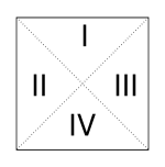
Figure 1: Mapping the symmetries (see text).

Figure (1) shows how the following symmetries can be used to map the elements in the top quadrant of the rotation matrix into each of the other quadrants. First,

$$d^{l}_{m,m^{\prime}}=(-1)^{m-m^{\prime}}d^{l}_{m,m^{\prime}},$$ (22)

which maps elements in region I into region II as shown in Figure 1. Next,

$$d^{l}_{m,m^{\prime}}=d^{l}_{-m^{\prime},-m},$$ (23)

which maps elements in region I into region III. And finally,

$$d^{l}_{m,m^{\prime}}=(-1)^{m-m^{\prime}}d^{l}_{-m,-m^{\prime}}.$$ (24)

This maps elements in region I into region IV. The relations (22) to (24) can be used in conjunction with Equation (21), to find all the elements of the Wigner $D$ functions from the values of $d^{l}_{m,m^{\prime}}$ in the upper quadrant. Similar, but more complicated, symmetry relations exist for the $D^{l}_{m,m^{\prime}}$.

For a given value of $l$ we can construct a sum of spherical harmonics in the coordinate system $S^{\prime}\{r,\theta^{\prime},\phi^{\prime}\}$ as follows

$$Y_{l}^{\prime}=\sum_{m^{\prime}}a^{\prime}_{l,m^{\prime}}Y_{l,m^{\prime}}(\theta^{\prime},\phi^{\prime}).$$ (25)

We can use this and the transformation in equation (20) to find the transformed sum, $Y_{l}$ in the coordinate system $S\{r,\theta,\phi\}$

$$Y_{l} = \sum_{m^{\prime}}a^{\prime}_{l,m^{\prime}}\left(\sum_{m}D^{l}_{m,m^{\prime}}(\alpha,\beta,\gamma)Y_{l,m}(\theta,\phi)\right)$$ (26)

$$= \sum_{m}\left(\sum_{m^{\prime}}a_{l,m^{\prime}}D^{l}_{m,m^{\prime}}(\alpha,\beta,\gamma)\right)Y_{l,m}(\theta,\phi)=\sum_{m}a_{l,m}Y_{l,m}(\theta,\phi)$$

This gives an expression for the rotated coefficients

$$a_{l,m}=\sum_{m^{\prime}}a_{l,m^{\prime}}D^{l}_{m,m^{\prime}}(\alpha,\beta,\gamma).$$ (27)

Finding the rotated coefficients therefore requires a simple matrix multiplication once the appropriate $D$ function is known. To apply this in practice one needs a fast and accurate way of generating the matrix elements $D^{l}_{m,m^{\prime}}$ for the rotation matrix. There are $(2l+1)^{2}$ elements needed to describe the rotation of each mode and the value of each element depends upon the particular values of $(\alpha,\beta,\gamma)$used for that rotation.

Varshalonich, Moskalev & Khersonskii (1988) provide a set of matrices for the $d^{l}_{m,m^{\prime}}(\beta)$ for the modes $l=1/2,1,3/2,\ldots,5$. For example, the case $l=1$ is

$$d^{1}_{m,m^{\prime}}(\beta)=\left(\begin{array}[]{cccc}\frac{1+\cos\beta}{2}&-\frac{\sin\beta}{\sqrt{2}}&\frac{1-\cos\beta}{2}\\ \frac{\sin\beta}{\sqrt{2}}&\cos\beta&-\frac{\sin\beta}{\sqrt{2}}\\ \frac{1-\cos\beta}{2}&\frac{\sin\beta}{\sqrt{2}}&\frac{1+\cos\beta}{2}\end{array}\right).$$ (28)

Fortunately, rather than working these matrices out by hand, Varshalovich et al. (1988) includes a set of iteration formulae, which, in conjunction with the symmetry relations for the $d^{l}_{m,m^{\prime}}$, can be used to generate matrices for the higher modes from the previous ones. The first iteration formula provides a way of generating an element in the mode $l+1$ by using the equivalent element in the matrices for the modes $l$ and $l-1$.

$$D^{l+1}_{m,m^{\prime}} = f\left(D^{l}_{m,m^{\prime}},D^{l-1}_{m,m^{\prime}}\right)$$ (29)

$$= (l+1)(2l+1)\left[-\frac{\sqrt{(l^{2}-m^{2})(l^{2}-m^{\prime 2})}D^{l-1}_{m,m^{\prime}}+\left(\cos\beta-\frac{m,m^{\prime}}{l(l+1)}\right)D^{l}_{m,m^{\prime}}}{\sqrt{((l+1)^{2}-m^{2})((l+1)^{2}-m^{\prime 2})}}\right].$$

Applying this formula repeatedly allows the central nine elements to be generated for all of the matrices.

Another iteration formula uses the values already in the matrix to calculate the element directly to the left. For example the element $D^{3}_{02}$ could be generated using the elements $D^{3}_{01}$ and $D^{3}_{00}$.

$$D^{l}_{m,m^{\prime}+1} = f\left(D^{l}_{m,m^{\prime}},D^{l}_{m,m^{\prime}-1}\right)$$ (30)

$$= \frac{2e^{-i\gamma}}{\sqrt{(l-m^{\prime})(l+m^{\prime}+1})}\times$$

$$\times\left[\frac{(-m+m^{\prime}\cos\beta)D^{l}_{m,m^{\prime}}}{\sin\beta}-\frac{1}{2}\sqrt{(l+m^{\prime})(l-m^{\prime}+1)}D^{l}_{m,m^{\prime}-1}e^{-i\gamma}\right].$$

Similar iteration functions exist to move up a matrix and across a matrix to the right.

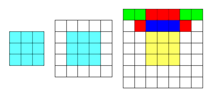
Figure 2: The basic steps involved in the iteration method described in the text for increasing matrix size: (left) $l$=1, (middle) $l=2$, and (right) $l$=3.

Figure (2) shows the iteration scheme. Iteration formula (29) is used to generate the elements coloured in yellow from the elements coloured in cyan. The elements coloured in yellow are then used to calculate the elements coloured in blue. The yellow and blue elements are used to calculate the elements coloured in red. The red elements are used to calculate the elements coloured in green. The symmetry relations are used to calculate the elements in the other three quadrants. Once the $l=3$ matrix has been calculated it can be used with the $l=2$ matrix to find the fourth matrix, and so on and so forth.

This method is fairly straightforward to implement but care is needed. The main problem with it is that the second iteration formula shown, equation (30) includes a term in which a factor is divided by $\sin\beta$. If $\beta\simeq 0$ or $\beta\simeq\pi$ then $\sin\beta\simeq 0$ leading to numerical problems.

An alternative approach is to calculate each $d^{l}_{mm^{\prime}}$ using factorials. The procedure encoded the definition of the $d^{l}_{m,m^{\prime}}$ given in Edmonds (1960):

$$d^{l}_{m,m^{\prime}}(\beta) = \left[\frac{(l+m^{\prime})!(l-m^{\prime})!}{(l+m)!(l-m)!}\right]^{\frac{1}{2}}\sum_{k}\left(\begin{array}[]{c}l+m\\ l-m^{\prime}-k\end{array}\right)\left(\begin{array}[]{c}l-m\\ k\end{array}\right)(-1)^{l-m^{\prime}-k}$$ (36)

$$\times\left(\cos\beta\right)^{2k+m^{\prime}+m}\left(\sin\beta\right)^{2l-2k-m^{\prime}-m}.$$

In this expression the variable $k$ varies between $0$ and the smallest of $l-m$ and $l-m^{\prime}$. This method avoids the problem of dividing through by $(\sin\beta)^{n}$ when $\beta$ is small. The results are far more stable and satisfy both of the techniques given above for testing the rotation code. The procedure can be tested using a random number generator to produce matrices for the full range of possible Euler angles.

There are two main tests that can be made of the results. First, the rotation code should generate the correct values for the $d^{l}_{m,m^{\prime}}$ matrices given in Varshalovich et al. (1988). Since the iteration formula are for the $D^{l}_{m,m^{\prime}}$ they will be applicable to the $d^{l}_{m,m^{\prime}}$ if $\alpha$ and $\gamma$ are set to zero. Choosing a value of $\beta$ and using it in matrices (25) and (26) should reproduce the precise calculation of the $l=3,4\textrm{ and }5$ matrices as given by Varshalovich et al. (1988). Second, the calculated matrices should be rotation matrices, so they should preserve the length of a vector. We define the vector of coefficients $A_{l}$ for a particular mode $l$ as

$$A_{l}=(a_{l,-l},a_{l,-l+1},\ldots,a_{l,-1},a_{l,0},a_{l,1},\ldots a_{l,l-1},a_{l,l})$$ (37)

and use this to define the length of $A_{l}$ to be

$$|A_{l}|=\sqrt{\sum_{m}|a_{l,m}|^{2}}.$$ (38)

The length should be preserved under the transformation. This allows the rotation code to be tested for any values of $l>5$ and for $\alpha,\gamma\neq 0$.

3.3 Implementation

In order to apply these ideas to make a test of CMB fluctuations, we first need a temperature map from which we can obtain a measured set of $a_{l,m}$. Employing equation 27 with some choice of Euler angles yields a rotated set of the $a_{l,m}$. It is straightforward to choose a set of angles such that random orientations of the coordinate axis can be generated. The Wigner $D$ function needed to compute this transformation is generated using the techniques described in Section 3.3. For the purposes of this paper we only compute the effect of rotation on low values of $l$. There is no difficulty in principle in extending this method to very high spherical harmonics, but the computational generation of Wigner $D$ scales by $\sim l^{2}$ so have chosen to limit ourselves to $l$=20. Once a rotated set has been obtained, Kuiper’s statistic is calculated from the relevant transformed set of phases. For each CMB map, 3000 rotated sets are calculated by this kind of resampling of the original data, producing 3000 values of $V_{\mathrm{cmb}}$. The values of the statistic are binned to form a measured (re-sampled) distribution of $V_{\mathrm{cmb}}$. The same procedure is applied to the 1000 Monte Carlo sets of $a_{l,m}$ drawn from a uniformly random distribution, i.e. each set is rotated 3000 times and a distribution of $V_{\mathrm{MC}}$ under the null hypothesis is produced. These realizations are then binned to created an overall global average distribution under the null hypothesis. In the following applications, the distribution of the 3000 values of V was split into 100 equally-spaced bins ranging from $V=0$ to 3.0 for different $l$ and 100 equally-spaced bins ranging from $V=0$ to 5.2 for different $m$.

In order to determine whether the distribution of $V_{\mathrm{cmb}}$ is compatible with a distribution drawn from a sky with random phases, we use a simple $\chi^{2}$ test, using

$$\chi^{2}=\sum_{i}\frac{(f_{i}-\overline{f_{i}})^{2}}{\overline{f_{i}}}$$ (39)

where the summation is over all the bins and $\overline{f_{i}}$ is the number expected in the $i$th bin from the overall average distribution. The larger the value of $\chi^{2}$ the less likely the distribution functions are to be drawn from the same parent distribution. Values of $\chi^{2}_{\mathrm{MC}}$ are calculated for the 1000 Monte Carlo distributions and $\chi^{2}_{\mathrm{cmb}}$ is calculated from the distribution of $V_{\mathrm{cmb}}$. If the value of $\chi^{2}_{\mathrm{cmb}}$ is greater than a fraction $p$ of the values of $\chi^{2}_{\mathrm{MC}}$, then the phases depart from a uniform distribution at significance level $p$. We have chosen 95 per cent as an appropriate level for the level at which the data are said to display signatures that are not characteristic of a statistically homogeneous Gaussian random field.

4 Applications

4.1 Toy Models

As a first check on the suitability of our method for detecting evidence of non-Gaussianity in CMB skymaps, sets of spherical harmonic coefficients were created with phases drawn from non-uniform distributions. Three types of distributions were used to test the method: (i) the phases were coupled (ii) the phases were drawn from a cardioid distribution and (iii) the phases were drawn from a wrapped Cauchy distribution; see Fisher (1993). The fake sets of coefficients were created in a manner that insured that the orthonormality of the coefficients were preserved as outlined in equations (9)–(11).

The first non–uniform distribution of phases is constructed using the following relationship

$$\phi_{m}=\phi_{m-1}+k$$ (40)

where $\phi_{m=-l}$ is a random number chosen between 0 and 2$\pi$. The results of the simulation with $k=1$ are shown in panel (i) of Tables 1 and 2. The sky is taken to be non-Gaussian if $\chi^{2}_{\rm sky}$ is larger than 95 % of $\chi^{2}_{MC}$ for a particular mode. The phase difference method should be particularly suited to detecting this kind of deviation from Gaussianity because the phase differences are all equal in this case; the distribution of phase differences is therefore highly concentrated rather than uniform. Nevertheless, the non-uniformity is so clear that it is evident from the phases themselves, even for low modes. On the other hand, assessing non-uniformity from the quadrupole mode $l=2$ on its own is difficult even in this case because of the small number of independent variables available.

The cardioid distribution was chosen because studies of phase evolution in the non-linear regime have shown phases rapidly move away from their initial values, however, they wrap around many multiples of 2$\pi$ and the ’observed’ phases appear random (Chiang and Coles 2000; Watts et al. 2003). This evolution can be distinguished by the phases differences which appear to be drawn from a roughly cardioid distribution (Watts et al. 2003). The cardioid distribution has a probability density function given by

$$f(\theta)=\frac{1}{2\pi}[1+2\rho\cos(\theta)],\quad 0\leq\theta<2\pi,0\leq\rho\leq 1/2,$$ (41)

where $\rho$ is the mean resultant length. As $\rho\rightarrow 0$ the distribution converges to a uniform distribution. The kurtosis of the distribution is given by

$$K=-\frac{\rho^{4}}{(1-\rho)^{2}}.$$ (42)

Sets of coefficients were produced from distributions with $\rho=0,0.2,0.4,0.5$. The distributions themselves were generated using rejection methods. The results are given in panel (ii) of Tables 1 and 2. The results with $\rho=0$ are not shown: they indicate the coefficients are taken from a Gaussian random field, as expected. Furthermore, with $\rho=0.5$ the non-uniformity detected in the phases and phase differences for $l=20$ is not particularly significant, however, the kurtosis for this distribution is not especially large.

		i	ii			iii
	$K$		-0.003	-0.07	-0.25	0.06	0.37	1.44	5.76	$\infty$
$l$
2		76	79	29	81	53	21	68	98	52
4		96	56	41	44	68	77	39	68	100
6		100	18	56	83	61	41	99	85	100
8		100	99	16	64	97	18	99	100	100
10		100	11	64	39	19	63	24	99	100
12		100	22	45	34	38	96	39	95	100
14		100	63	4	82	60	62	93	97	100
16		100	69	41	31	16	68	72	100	100
18		100	83	63	44	54	18	100	100	100
20		100	5	72	95	64	1	83	100	100

Table 1: Results for non-Gaussian skies based on phases between consecutive values of $m$ at a fixed $l$. The results show the significance levels of detected departures from random phases for simulated distributions corresponding to (i) coupled phases, (ii) a Cardioid distribution and (iii) a wrapped Cauchy distribution. In the latter two cases various parameter choices are shown as described in the text. These results are obtained from 1000 Monte Carlo skies.

		i	ii			iii
	$K$		-0.003	-0.07	-0.25	0.06	0.37	1.44	5.76	$\infty$
$l$
2		67	81	63	90	52	46	37	98	35
4		97	68	41	12	79	89	28	69	100
6		100	18	66	87	25	4	98	95	100
8		100	98	69	8	74	87	99	100	100
10		100	34	66	12	44	32	65	99	100
12		100	37	80	71	58	7	55	72	100
14		100	22	29	85	79	40	28	65	100
16		100	48	78	88	43	78	89	99	100
18		100	8	5	23	84	19	100	100	100
20		100	85	55	99	53	27	32	99	100

Table 2: Results for non-Gaussian skies based on phase differences between consecutive values of $m$ at a fixed $l$. The results show the significance levels of detected departures from random phases for simulated distributions corresponding to (i) coupled phases, (ii) a cardioid distribution and (iii) a wrapped Cauchy distribution. In the latter two cases various parameter choices are shown as described in the text. These results are obtained from 1000 Monte Carlo skies.

Phases were drawn from wrapped Cauchy distributions in order to test the method against skies with larger values of kurtosis. The wrapped Cauchy distribution has a probability density function given by

$$f(\theta)=\frac{1}{2\pi}\;\frac{1-\rho^{2}}{1+\rho^{2}-2\rho\cos(\theta)},\quad 0\leq\theta<2\pi,0\leq\rho\leq 1$$ (43)

The kurtosis is given by

$$K=\frac{(\rho^{2}-\rho^{4})}{(1-\rho)^{2}}.$$ (44)

As $\rho\rightarrow 0$ the distribution tends towards a uniform distribution. As $\rho\rightarrow 1$ the distribution tends towards a distribution concentrated at $\phi=0$. Fisher (1993) gives a method for simulating the distribution. Sets of coefficients were created for $\rho=0,0.2,0.4,0.6,0.8,1$. The results are given in panel (iii) of Tables 1 and 2. Again $\rho=0$ is not displayed, but was used to check the distribution simulation was correct because it should correspond to a uniformly random distribution. For $\rho\geq 0.6$ the coefficients are distinctly non–Gaussian. The results in the Table indicate that the method can pick out departures from uniformly random phase distributions, at 95% confidence level for $|K|\ga 1$. Note also that the results from $\rho=1$ demonstrate that firm conclusions about the Gaussianity and/or stationarity of the sky are difficult to draw using the quadrupole alone. Even for the highly non–Gaussian distribution with $K=\infty$, our statistic does not prove to be discriminatory. In summary, however, the tests do show that the method can pick out departures from the random phase hypothesis in CMB sky maps using low multipole modes.

4.2 Quadratic Non-Gaussian Maps

In order to further examine the performance of our statistic, we applied it to non-Gaussian models with stronger physical foundations. At large scales, the CMB is dominated by the Sachs-Wolfe (Sachs & Wolfe 1967) effect so that the temperature fluctuations are proportional to fluctuations in the gravitational potential on the last scattering surface. Non-Gaussian CMB skies can be generated by introducing a non-linear term in the gravitational potential $\Phi(n)$

$$\Phi(n)=\Phi_{L}(n)+f_{nl}(\Phi^{2}_{L}(n)-<\Phi^{2}_{L}(n)>)$$ (45)

where $\Phi_{L}(n)$ refers to the linear part of the potential, $f_{nl}$ is the non-linear parameter controlling the amount of non-Gaussianity and the brackets indicate a volume average (Liguori, Matarrese & Moscardini 2003). We applied our method to these types of skies with varying levels of non-Gaussianity controlled by the parameter $f_{nl}$.

The results for the most extreme form of non-Gaussianity ($f_{nl}=\infty$) are shown in panel (i) in Tables 3 and 4. Note that our statistic is clearly unsuitable for detecting this form of non-Gaussianity. Even for this level of non-Gaussianity the method is incapable of finding any deviations of the phases or phase differences from the random phase hypothesis. The reason for this is the very simple form of phase association we are testing here does not pick up very sensitively the quadratic correlations manifested by the model given in equation (40); see Watts & Coles (2003). We discussed this in Section 2.1, in the context of Fourier phases. The reason for this failure is that the method we are using is much more sensitive to departures from statistical homogeneity over the celestial sphere than it is to statistically homogeneous non–Gaussianity. To put this another way, our method will only be sensitive to departures from Gaussian behaviour, such as localized edges or blobs, if these features occupy a substantial fraction of the celestial sphere. This result will be useful later on, when we interpret the results we obtain from real data.

It is also worth mentioning that it would not surprising if a large significance level were attached to one of the $D_{l}(m)$ values even if the null hypothesis were correct. Since we are looking at 18 values of $m$ when scanning across fixed values of $m$, statistically speaking, one value of $m$ should lead to a probability value larger than 95 per cent. We will not try to assess the significance level of any departure from the null hypothesis in the context of this result as our motivation for introducing this form of non–Gaussianity is basically to show that our method struggles to detect it. Whatever method one uses to combine probabilities across modes would clearly produce a marginal result in this case for the probability that there is any departure at all. We will explore this question in more detail in future work (Dineen et al., in prep.).

		$\phi_{m}(l)$					$D_{m}(l)$
$l$		i	ii	iii	iv		i	ii	iii	iv
2		89	25	1	7		42	19	1	12
4		67	56	55	69		10	43	40	43
6		13	93	94	94		89	94	94	91
8		88	31	9	31		31	35	38	30
10		69	12	12	30		88	16	46	43
12		81	97	89	73		21	94	81	90
14		53	77	94	94		93	95	96	96
16		76	100	100	99		92	97	97	94
18		43	47	84	67		56	19	86	68
20		23	63	26	5		5	24	19	7

Table 3: Results based on phases and phase differences between consecutive values of $m$ at a fixed $l$. The results show the significance levels of detected departures from random phases for (i) the quadratic non-Gaussian map ($f_{nl}=\infty$), (ii) the ILC map, (iii) the cleaned TOH map and (iv) the Wiener filtered TOH map.

		$D_{l}(m)$
$m$		i	ii	iii	iv
1		69	31	59	10
2		92	75	36	46
3		63	23	35	67
4		37	81	72	44
5		43	4	2	74
6		10	4	46	34
7		97	79	87	55
8		59	29	62	43
9		49	68	54	18
10		84	17	79	81
11		62	41	37	85
12		88	6	85	78
13		25	76	65	60
14		58	2	53	49
15		76	50	35	15
16		86	48	16	28
17		94	24	71	84
18		39	82	63	49

Table 4: Results based on phase differences between consecutive values of $l$ at a fixed $m$. The results show the significance levels of detected departures from random phases for (i) the quadratic non-Gaussian map ($f_{nl}=\infty$), (ii) the ILC map, (iii) the cleaned TOH map and (iv) the Wiener filtered TOH map.

4.3 The COBE DMR data

We now discuss the application of our method to real data in order to see if any signs of non-random phases could be found in published sky maps. In this subsection we look at the $a_{l,m}$ obtained from COBE-DMR data and in the next subsection we apply the method to $a_{l,m}$ obtained from three all-sky maps derived from WMAP data.

The DMR (Differential Microwave Radiometer) instrument on board the COBE satellite ushered in the era of precision cosmology by measuring primordial temperature fluctuations of order $\Delta T/T=10^{-5}$ in the cosmic microwave background (CMB) radiation. The DMR instrument comprised six differential microwave radiometers: two nearly independent channels, labelled A and B, at frequencies 31.5, 53 and 90 GHz. The data from all three frequencies have been used to calculate the $a_{l,m}$ corresponding to the CMB signal from regions outside the Galactic cut. To keep the presentation brief we discuss the behaviour of $a_{l,m}$ for only the even modes.

The results of the application of the method on the $a_{l,m}$ are displayed in Table 5. The method was applied to five realisations (rotations) of the DMR sky in order to examine whether the results were stable and consequently whether the conclusions were robust. In the Table it is clear that the large values of $\chi^{2}$ (and consequently large significance levels) do indeed appear stable but lower values (when the phases appear random) the probabilities depend stronly upon the realisation. However, we are only interested in significance levels that are larger than 95% and these appear stable for all realisations.

The statistic indicates that both the phases and phase differences of $l=10$ mode appear inconsistent with the random phase hypothesis. For all 5 realisations, the $\chi^{2}$ values are larger than 95% of the MC skies. Figure 3 shows the distribution of $V$ obtained for realisation 1 from Table 5 compared with the average distribution of the MC skies for $l=10$ and 12. The distribution of $D_{m}(10)$ clearly differs from that of the random phase MC skies whereas $D_{m}(12)$ appears by eye to be drawn form the same distribution. The results in Table 5 also show that the phases obtained from the $l=18$ also appear non-random, but the confidence of this result is dependent on the realisation.

		$\phi_{m}(l)$						$D_{m}(l)$
$l$		1	2	3	4	5		1	2	3	4	5
2		35	40	46	46	47		38	38	45	40	34
4		81	83	81	83	79		78	76	76	78	78
6		49	31	52	53	76		46	44	43	37	41
8		19	43	14	41	1		68	63	67	65	63
10		97	97	97	98	97		96	96	96	96	96
12		49	38	1	1	59		13	24	14	3	7
14		61	77	33	31	35		3	10	77	8	10
16		4	77	87	92	39		57	66	67	59	65
18		97	94	94	96	97		92	92	91	94	93
20		64	58	7	51	36		30	19	18	30	23

Table 5: Results for COBE DMR data based on phases and phase differences between consecutive values of $m$ at a fixed $l$. The method was applied to 5 realisations of the DMR sky in order to demonstrate the stability of the results.

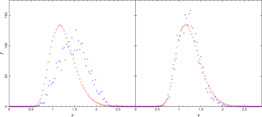
Figure 3: Examples of the distribution of Kuiper’s statistic V for $D_{m}(10)$ (left) and $D_{m}(12)$ (right) in the COBE-DMR data. The red squares and blue stars correspond to the average distribution of V for the 1000 MC skies and the distribution for the DMR data respectively.

The issue of non-Gaussianity in the COBE-DMR data has been controversial (Ferreira, Magueijo & Gorski 1998; Bromley & Tegmark 1999; Magueijo 2000), but is likely to involve systematic problems identified in the data set we use. Note however that the strong detection we have found is at a different harmonic mode $l=10$ than that originally claimed by Ferreira et al. (1998) who used a diagnostic related to the bispectrum. There need not be a conflict here because, as we discussed above, we are not sensitive to the same form of phase correlations in this method as the bispectrum.

We do not wish to go further into the statistical properties of the COBE-DMR data here. The results we have presented are from the original data which is now known to have suffered from some systematic problems (Banday, Zaroubi & Gorski 2000). The effect we are seeing is therefore probably not primordial, making this largely an academic discussion. The data have also partly been superseded by WMAP. It does, however, illustrate the importance of using complementary approaches to identify all possible forms of behaviour in data sets even when they are of experimental, rather than cosmological, origin.

4.4 WMAP results

The WMAP instrument comprises 10 differencing assemblies (consisting of two radiometers each) measuring over 5 frequencies ($\sim$23, 33, 41, 61 and 94 GHz). The WMAP team have released an internal linear combination (ILC) map that combined the five frequency band maps in such a way to maintain unit response to the signal CMB while minimising the foreground contamination. The construction of this map is described in detail in Bennett et al. (2003). To further improve the result, the inner Galactic plane is divided into 11 separate regions and weights determined separately. This takes account of the spatial variations in the foreground properties. The final map covers the full-sky and should represent only the CMB signal, although it is not anticipated that foreground subtraction is perfect.

The WMAP ILC map is issued with estimated errors in the map-making technique. This uncertainty could be included in the Monte Carlo simulations of the null hypothesis used to construct sampling distributions of our test statistic. This would be difficult to do rigorously as errors are highly correlated, but is possible in principle. We have decided not to include the experimental errors in this analysis because it is just meant to illustrate the method: a more exhaustive search for CMB phase correlations (for which such considerations would be relevant) will have to wait for cleaner maps than are available now.

Following the release of the WMAP 1 yr data Tegmark, de Oliveira-Costa & Hamilton (2003; TOH) have produced a cleaned CMB map. They argued that their version contained less contamination outside the Galactic plane compared with the internal linear combination map produced by the WMAP team. The five band maps are combined with weights depending both on angular scale and on the distance from the Galactic plane. The angular scale dependence allows for the way foregrounds are important on large scales whereas detector noise becomes important on smaller scales. TOH also produced a Wiener filtered map of the CMB that minimisizes rms errors in the CMB. Features with a high signal-to-noise are left unaffected, whereas statistically less significant parts are suppressed. While their cleaned map contains residual Galactic fluctations on very small angular scales probed only by the W band, these fluctuations vanish in the filtered map.

The three all-sky maps are available in HEALPix format (Gorski, Hivon & Wandelt 1999). We derived the $a_{l,m}$ for each map using the anafast routine in the HEALPix package. The results are shown in panels (ii) to (iv) in Tables 3 and 4. The results for the ILC map suggest there are departures from the random phase hypothesis for the phases of $l=12$ and 16 and the phase differences for $l$=14 and 16. The departure for $l$=16 appears very strong with the $\chi^{2}$ value being larger than 995 of the values obtained for the MC skies. For these data we have also explored the effect of measuring differences between the phases at different $l$ for the same value of $m$. (We did not present results in this case for the COBE-DMR data, as we only discussed the even $l$-modes in that case and differences between adjacent $l$ would require every mode.) Notice that the confidence levels of non-uniformity are larger for $D_{m}$ at fixed $l$ than for $D_{l}$ at fixed $m$. This is an interesting feature of the WMAP data.

To investigate this mode further we therefore reconstructed the temperature pattern on the sky solely using only the spherical harmonic modes for $l=16$ with their appropriate $a_{l,m}$ and compared this with a map with the same power spectrum but with random phases (figure 4). The result is a striking confirmation of the above argument that our method is very sensitive to departures from statistical homogeneity. The $l=16$ modes are clearly forming a more structured pattern than the random-phase counterpart. The alignment of these modes with the Galactic plane is striking; it may be that the angular scale corresponding to $l=16$ may relate to the width of the zones used to model the Galactic plane.

The two maps produced by Tegmark et al. (2003; TOH) also suggest that the phases for the $l=16$ scale are non-random. The cleaned map shows departures from the random phase hypothesis at greater than 95% confidence for the phases of $l$=16 and phase differences of $l=14$ and 16. The Wiener filtered map finds departures for the phases corresponding to $l=16$ and phase differences in $l$=14. Both the cleaned and the Wiener filtered maps of TOH display similar band patterns to that observed in the $l=16$ map for the ILC; we show the Wiener filtered TOH map for comparison.

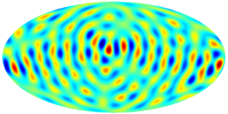
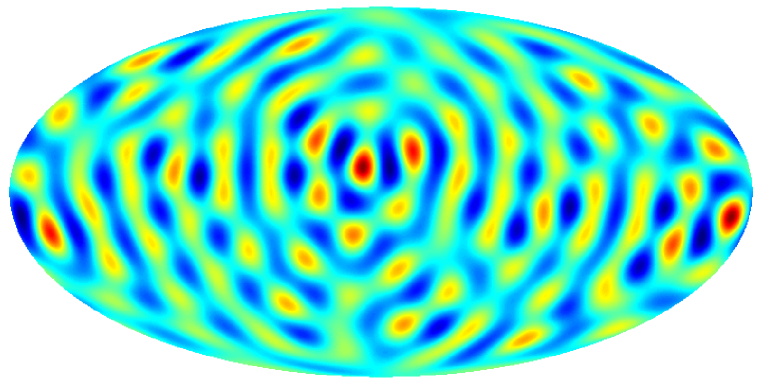
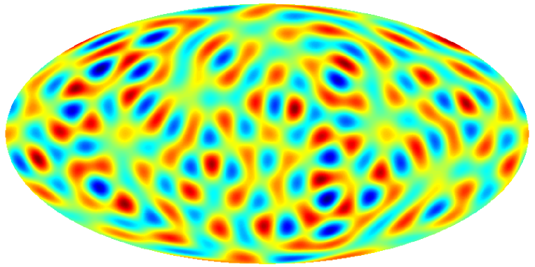
Figure 4: Top: Internal linear combination map constructed with $a_{l,m}$ for $l=16$ only. Middle: The TOH Wiener-filtered map with $a_{l,m}$ for $l=16$ only. Bottom: A random-phase realization of the map including modes with $l=16$ only.

The morphological appearance of these fluctuations as a band across the Galactic plane may be indicative of residual foreground still present in the CMB map after subtraction. This is the most likely explanation for the alignment of features relative to the Galactic coordinate system, since the scanning noise is not aligned in this way. Further evidence for this is provided by Naselsky et al. 2003 from cross–correlations of the phases of CMB maps with various foreground components. In any case one should certainly caution against jumping to the conclusion that this represents anything primordial. These are preliminary data with complex variations in signal-to-noise across the sky. Nevertheless, the results we present here do show that the method we have presented is useful for testing realistic observational data for departures from the standard cosmological statistics.

5 Discussion and Conclusions

In this paper we have presented a new method of testing CMB data for departures from the homogeneous statistical behaviour associated with Gaussian random fields generated by inflation. Our method uses some of the information contained within the phases of the spherical harmonic modes of the temperature pattern and is designed to be most sensitive to departures from stationarity on the celestial sphere. The method is relatively simple to implement, and has the additional advantage of being performed entirely in “data space”. Confidence levels for departures from the null hypothesis are calculated forwards using Monte Carlo simulations rather than by inverting large covariance matrices. The method is non-parametric and, as such, makes no particular assumptions about data. The main statistical component of our technique is a construction known as Kuiper’s statistic, which is a kind of analogue to the Kolmogorov-Smirnov test, but for circular variates.

In order to illustrate the strengths and weaknesses of our approach we have applied it to several test data sets. To keep computational costs down, but also to demonstrate the usefulness of non-parametric approaches for small data sets, we have concentrated on low–order spherical harmonics.

We first checked the ability of our method to diagnose non-uniform phases of the type explored by Watts, Coles & Melott (2003) and Matsubara (2003). The method is successful even for the low–order modes that have few independent phases available. We then applied the method to quadratic non–Gaussianity fields of the form discussed by Watts & Coles (2003) and Liguori, Matarrese & Moscardini (2003). Our method is not sensitive to the particular form of phase correlation displayed by such fields as, although non–Gaussian, they are statistically stationary. Phase correlations are present in such fields, but do not manifest themselves in the simple phase or phase-difference distributions discussed in this paper. These two examples demonstrate that our method is a useful diagnostic of statistical non-uniformity and its applicability to non–Gaussian fields is likely to be restricted to cases where the pattern contains strongly localized features, such as cosmic strings or textures (e.g. Contaldi et al. 2000).

We next turned our attention to the COBE–DMR data. Claims and counter-claims have already been made about the possible non–Gaussian nature of these data, the most likely explanation of the observed features being some form of systematic error. Our test does show up non-uniformity in the phase distribution at high confidence levels for the $l=10$ mode and, less robustly, at $l=18$. This is a different signal to that claimed previously to be indicative of non–Gaussianity. Its interpretation remains unclear.

Finally we applied our method to various representations of the WMAP preliminary data release. In this case we find clear indications at $l=16$ and, less significantly, at $l=14$. The distribution of the $l=16$ harmonics on the sky shows that this result is not a statistical fluke. The data are clearly different from a random–phase realisation with the same amplitudes and there is certainly the appearance of some correlation of this pattern with the Galactic coordinate system. We are not claiming that this proves there is some form of primordial non–Gaussianity in this dataset. Indeed the WMAP data come with a clear warning its noise properties are complex so it would be surprising if there were no indications of this in the preliminary data. It will be useful to apply our method to future releases of the data in order to see if the non-uniformity of the phase distribution persists as the signal-to-noise improves. At the moment, however, the most plausible interpretation of our result is that it represents some kind of Galactic contamination, consistent with other (independent) claims (Dineen & Coles 2003; Chiang et al. 2003; Eriksen et al. 2003; Naselsky et al. 2003).

As a final comment we mention that the aptitude of our method for detecting spatially localised features (or departures from statistical homogeneity generally) suggests that it is may be useful as a diagnostic of the repeating fluctuation pattern produced on the CMB sky in cosmological models with compact topologies (Levin, Scannapieco & Silk 1998; Scannapieco, Levin & Silk 1999; Rocha et al. 2002); see Levin (2002) for a review. We shall return to this issue in future work.

References

- [] Albrecht A., Steinhardt P.J., 1982, Phys. Rev. Lett., 48, 1220
- [] Banday A.J., Zaroubi S., Gorski K.M., 2000, ApJ, 533, 575
- [] Bardeen J.M., Bond J.R., Kaiser N., Szalay A.S., 1986, ApJ, 304, 15
- [] Bartolo N., Matarrese S., Riotto, A., 2002, Phys. Rev. D. 65, 103505
- [] Bennett C.L. et al., 1996, ApJ, 464, L1
- [] Bennett C.L. et al., 2003, ApJ, 538, 1
- [] Bennet C.L. et al., 2003, ApJS, 148, 1
- [] Bond J.R., Efstathiou G., 1987, MNRAS, 226, 655
- [] Bromley B.C., Tegmark M., 1999, ApJ, 524, L79
- [] Chiang L.-Y., 2001, MNRAS, 325, 405
- [] Chiang L.-Y., Coles P., 2000, MNRAS, 311, 809
- [] Chiang L.-Y., Coles P., Naselsky P.D., 2002, MNRAS, 337, 488
- [] Chiang L.-Y., Naselsky P.D., Coles P., 2002, astro-ph/0208235
- [] Chiang L.-Y., Naselsky P.D., Verkhodanov O.V., Way M.J., 2003, ApJ, 590, L65
- [] Coles P., Barrow J.D., 1987, MNRAS, 228, 407
- [] Coles P., 1988, MNRAS, 234, 509
- [] Coles P., Jones B.J.T., 1991, MNRAS, 248, 1
- [] Coles P, Chiang L.Y., 2000, Nat, 406, 376
- [] Colley W.N., Gott J.R., 2003, MNRAS, 344, 686
- [] Contaldi C.R., Bean R., Magueijo J., 2000, Phys. Lett. B., 468, 189
- [] Contaldi C.R., Ferreira P.G., Magueijo J., Gorski K.M., 2000, ApJ, 534, 25
- [] Cooray A., 2001, Phys. Rev. D., 64, 043516
- [] Dineen P., Coles P., 2003, MNRAS, in press, astro-ph/0306529
- [] Edmonds A.R., 1960, Angular Momentum in Quantum Mechanics, 2nd Edition. Princeton University Press, Princeton.
- [] Eriksen H.K., Hansen F.K., Banday A.J., Gorski K.M., Lilje P.B., 2003, astro-ph/0307507
- [] Ferreira P.G., Magueijo J., Gorski K.M., 1998, ApJ, 503, L1
- [] Fisher N.I., 1993, Statistical Analysis of Circular Data. Cambridge University Press, Cambridge.
- [] Gangui A., Martin J., Sakellariadou M., 2002, Phys. Rev. D. 66, 083502
- [] Gangui A., Pogosian L., Winitzki S., 2001, Phys. Rev. D. 64, 043001
- [Gorski, Hivon & Wandelt 1998] Górski K.M., Hivon E., Wandelt B.D., 1999, in Proceedings of the MPA/ESO Conference Evolution of Large-Scale Structure, eds. A.J. Banday, R.S. Sheth and L. Da Costa, PrintPartners Ipskamp, NL, pp. 37-42 (also astro-ph/9812350)
- [] Gupta S., Berera A., Heavens A.F., Matarrese S., 2002, Phys. Rev. D., 66, 043510
- [] Guth A.H., 1981, Phys. Rev. D., 23, 347
- [] Guth A.H., Pi S.-Y., 1982, Phys. Rev. Lett., 49, 1110
- [] Hansen F.K., Marinucci D., Vittorio N., 2003, Phys. Rev. D., 67, 123004
- [] Heavens A.F., 1998, MNRAS, 299, 805
- [] Hikage C., Matsubara T., Suto Y., 2003, ApJ submitted.
- [] Hinshaw G.F. et al., 2003, ApJS, 148, 135
- [] Hu W., 2001, Phys. Rev. D., 64, 083005
- [] Jain B., Bertschinger E., 1996, ApJ, 456, 43
- [] Jain B., Bertschinger E., 1998, ApJ, 509, 517
- [] Komatsu E., et al., 2002, ApJ, 566, 19
- [] Komatsu E., et al., 2003, ApJS, 148, 119
- [] Kuiper N.H., 1960, Koninklijke Nederlandse Akademie Van Wetenschappen, Proc. Ser. A, LXIII, pp. 38-49
- [] Levin J., 2002, Phys. Rep., 365, 251
- [] Levin J., Scannapieco E., Silk J., 1998, Phys. Rev. D., 58, 103516
- [] Liguori M., Matarrese S., Moscardini L., 2003, ApJ, 597, 57
- [] Linde A.D., 1982, Phys. Lett. B., 108, 389
- [] Linde A.D., Mukhanov V., 1997, Phys. Rev. D., 56, 535
- [] Luo X, 1994, ApJ, 427, L71
- [] Magueijo J., 2000, ApJ, 528, L57
- [] Martin J., Riazuelo A., Sakellariadou M., 2000, Phys. Rev. D., 61, 083518
- [] Matarrese S., Verde L., Heavens A.F., 1997, MNRAS, 290, 651
- [] Matarrese S., Verde L., Jimenez R., 2000, ApJ, 541, 10
- [] Matsubara T., 2003, ApJ, 591, L79
- [] Naselsky P.D., Verkhodanov O.V., Chiang L.-Y., Novikov I.D., 2003, ApJ, submitted, astro-ph/0310235
- [] Pando J., Valls-Gabaud D., Fang L., 1998, Phys. Rev. Lett., 81, 4568
- [] Peebles P.J.E., 1980, The Large-scale structure of the Universe. Princeton University Press, Princeton.
- [] Phillips N.G. Kogut A., 2001, ApJ, 548, 540
- [] Rocha G., Cayon L., Bowen R., Canavezes A., Silk J, Banday A.J., Gorski K.M., 2002, MNRAS, submitted, astro-ph/0205155
- [] Ryden B.S., Gramann M., 1991, ApJL, 383, L33
- [] Sachs R.K., Wolfe A.M., 1967, ApJ, 147, 73
- [] Sandvik H.B., Magueijo J., 2001, MNRAS, 325, 463
- [] Santos M.G. et al., 2001, Phys. Rev. Lett., 88, 241302
- [] Scannapieco E., Levin J., Silk J., 1999, MNRAS, 303, 797
- [] Scherrer R.J., Melott A.L., Shandarin S.F., 1991, ApJ, 377, 29
- [] Scoccimarro R., Colombi S., Fry J.N., Frieman J.A., Hivon E., Melott A.L., 1998, ApJ, 496, 586
- [] Smoot G.F. et al., 1992, ApJ, 396, L1
- [] Soda J., Suto Y., 1992, ApJ, 396, 379
- [] Starobinsky A.A., 1979, Pis’ma Zh. Eksp. Teor. Fiz., 30, 719
- [] Starobinsky A.A., 1980, Phys. Lett. B., 91, 99
- [] Starobinsky A.A., 1982, Phys. Lett. B., 117, 175
- [] Stirling A.J., Peacock J.A., 1996, MNRAS, 283, L99
- [] Tegmark M., de Oliveira-Costa A., Hamilton A.J.S., 2003, astro-ph/0302496
- [] Varshalovich D.A., Moskalev A.N., Khersonskii V.K., 1988, Quantum Theory of Angular Momentum. World Scientific, Singapore.
- [] Verde L., Heavens A.F., 2001, ApJ, 553, 14
- [] Verde L, Jimenez R., Kamionkowski M., Matarrese S., 2001, MNRAS, 325, 412
- [] Verde L, Wang L., Heavens A.F., Kamionkowski M., 2000, MNRAS, 313, 141
- [] Verde L. et al. 2002, MNRAS, 335, 432
- [] Watts P.I.R., Coles P., 2003, MNRAS, 338, 806
- [] Watts P.I.R., Coles P., Melott A.L., 2003, ApJ, 589, L61