The Sizes and Kinematic Structure of Absorption Systems Towards the Lensed Quasar APM08279+5255.

We have obtained spatially resolved spectra of the $z_{\rm em}=3.911$ triply imaged QSO APM08279+5255 using the Space Telescope Imaging Spectrograph (STIS) on board the Hubble Space Telescope (HST). We study the line of sight equivalent width (EW) differences and velocity shear of high and low ionization absorbers (including a damped Lyman alpha [DLA] system identified in a spatially unresolved ground based spectrum) in the three lines of sight. The combination of a particularly rich spectrum and three sight-lines allow us to study 27 intervening absorption systems over a redshift range $1.1<z_{\rm abs}<3.8$, probing proper transverse dimensions of 30 $h_{70}^{-1}$ pc up to 2.7 $\leavevmode\nobreak\ h_{70}^{-1}$ kpc. We find that high ionization systems (primarily C IV absorbers) do not exhibit strong EW variations on scales $<0.4$  $\leavevmode\nobreak\ h_{70}^{-1}$ kpc; their fractional EW differences are typically less than 30%. When combined with previous work on other QSO pairs, we find that the fractional variation increases steadily with separation out to at least $\sim 100$ $\leavevmode\nobreak\ h_{70}^{-1}$ kpc. Conversely, low ionization systems (primarily Mg II absorbers) show strong variations (often $>80$%) over kpc scales. A minimum radius for strong (EW $>0.3$ Å) Mg II systems of $>1.4$ $\leavevmode\nobreak\ h_{70}^{-1}$ kpc is inferred from absorption coincidences in all lines of sight. For weak Mg II absorbers (EW $<0.3$ Å), a maximum likelihood analysis indicates a most probable coherence scale of 2.0 $\leavevmode\nobreak\ h_{70}^{-1}$ kpc for a uniform spherical geometry, with 95% confidence limits ranging between 1.5 and 4.4 $\leavevmode\nobreak\ h_{70}^{-1}$ kpc. The weak Mg II absorbers may therefore represent a distinct population of smaller galaxies compared with the strong Mg II systems which we know to be associated with luminous galaxies whose halos extend over tens of kpc. Alternatively, the weak systems may reside in the outer parts of larger galaxies, where their filling factor may be lower. By cross-correlating spectra along different lines of sight, we infer shear velocities of typically less than 20 km s^-1 for both high and low ionization absorbers. Finally, for systems with weak absorption that can be confidently converted to column densities, we find constant $N$(C IV)/$N$(Si IV) across the three lines of sight. Similarly, the [Al/Fe] ratios in the $z_{\rm abs}=2.974$ DLA are consistent with solar relative abundances over a transverse distance of $\sim 0.35$ $\leavevmode\nobreak\ h_{70}^{-1}$ kpc.

1 Introduction

The study of high redshift absorption line systems in the lines of sight (LOS) to lensed and multiple QSOs can yield information on the sizes of intervening galaxies and the structure of the intergalactic medium (IGM). Statistical analyses of the Ly$\alpha$ forest in multiple LOS have established that the coherence length of Ly$\alpha$ absorbers ranges from a few pc to hundreds of kpc (e.g. Crotts 1989; Smette et al 1995; Petry, Impey & Foltz 1998; Petitjean et al. 1998; Lopez, Hagen & Reimers 2000; Rauch et al. 2001b). A significant fraction of Ly$\alpha$ forest clouds with neutral hydrogen column densities greater than $\log N$(H I)$>14$ (where $N$(H I) is measured in cm^-2) have associated metals detected primarily via highly ionized species such as C IV, even out to very high redshifts (Ellison et al 2000; Songaila 2001; Pettini et al. 2003). From studies of small scale variations using lensed QSOs, these high ionization metal systems have been found to exhibit little structure on transverse scales of a few pc (Rauch, Sargent & Barlow 1999). However, on kpc scales variations can be seen between in some absorption components (e.g. Smette et al 1995; Rauch, Sargent & Barlow 2001a); recently Tzanavaris & Carswell (2003) have inferred sizes of $\sim 0.5-8$ $\leavevmode\nobreak\ h_{70}^{-1}$ kpc for individual C IV clouds . Observations of multiple QSOs extend this type of analysis to larger scales and indicate that coherence (i.e. coincidence) between C IV systems still exists over dimensions of $\sim$ 100 $\leavevmode\nobreak\ h_{70}^{-1}$ kpc (e.g. Petitjean et al 1998; Lopez, Hagen & Reimers 2000). A complementary study of C IV absorbers in the vicinity of Lyman break galaxies has shown that the regions where metals are dispersed into the IGM probably extend over hundreds of kpc (Adelberger et al. 2003).

Compared with the results of the Ly$\alpha$ forest and high ionization absorbers, the structural properties of the galactic halos probed by low ionization metal line systems are relatively few. This is mainly due to the fact that low ionization absorbers have a lower incidence per unit redshift than Ly$\alpha$ or C IV systems. Rauch et al. (2002) probed four pairs of low ionization systems and found significant spatial and column density differences for individual components on scales of a few hundred pc, although in every case the absorber covered both LOS indicating that low ionization halos have overall dimensions larger than $\sim 0.5$ kpc. Kobayashi et al. (2002) studied the probable damped Ly$\alpha$ system (DLA) at $z_{\rm abs}=2.974$ towards APM08279+5255 and again found structural differences in the Mg II lines over scales of $\sim 0.3$ kpc. Using a spatially unresolved HIRES spectrum of APM08279+5255 Petitjean et al. (2000) inferred sub-kpc sizes for some Mg II systems based on partial coverage arguments. Churchill et al (2003) found evidence for minor structural differences on even smaller scales, although these are not reflected in discernable chemical abundance variations over distances of $0.135$ kpc in a DLA at $z_{\rm abs}=1.3911$. Indirect determinations of the size of Mg II systems, based on impact parameters and number density per unit redshift, indicate dimensions $\sim$ 50 $\leavevmode\nobreak\ h_{70}^{-1}$ kpc (Steidel 1995; Bergeron and Boissé 1991). Such large sizes have been claimed even for relatively weak absorbers (Churchill & LeBrun 1998; Churchill et al 1999).

Taken together, these observations indicate that the coherence length of C IV systems is much larger than that of Mg II systems. This is qualitatively consistent with the simple picture—drawn more than a decade ago from the incidence of these absorbers per unit redshift—of clumpy, low ionization, gas embedded in larger, more homogeneous, and more highly ionized outer halos (e.g. Steidel 1993). However, the number of multiple QSOs in which the transverse spatial dimensions of metal lines (particularly low ionization systems) have been determined is still relatively small. Moreover, the range of linear scales probed is somewhat limited, largely because ground-based spectroscopy requires image separations typically greater than 0.8  arcsec.

Here we present new spatially resolved observations of the triply imaged QSO $z_{\rm em}=3.911$ APM08279+5255 obtained with the Space Telescope Imaging Spectrograph (STIS) on board the Hubble Space Telescope (HST). The unique triple nature of this system has been recently confirmed by Lewis et al. (2002b) using a subset of these STIS data and can be explained as lensing by a naked cusp, probably associated with a highly inclined disk (Lewis et al. 2002a). In Figure 1 we reproduce a NICMOS image of APM08279+5255 obtained by Ibata et al. (1999), illustrating the configuration of the lensed images. APM08279+5255 is a particularly powerful case for probing the transverse dimensions of QSO absorbers for two reasons. First, its triple nature provides us with three times as many baselines as the more common QSO pairs. Second, its absorption spectrum is particularly rich in intervening (as well as associated) systems (Ellison et al 1999a,b), including a DLA at $z_{\rm abs}=2.974$ (Petitjean et al. 2000). The number of cases in which DLAs have been probed with multiple LOS is still relatively small (see Smette et al. 1995; Zuo et al 1997; Boissé et al. 1998; Lopez et al. 1999; Gregg et al. 2000; Churchill et al. 2003; Wucknitz et al. 2003).

In this paper we adopt a $\Omega_{M}=0.3$, $\Omega_{\Lambda}=0.7$, $H_{0}=70$ km s^-1 Mpc^-1 cosmology throughout, unless otherwise stated. In calculating the transverse distances corresponding to the angular separations of the lensed images of APM08279+5255, we adopt a redshift $z_{\rm lens}=1.062$ for the lensing galaxy which has so far remained undetected. This is the redshift of a strong, low ionization, absorption system revealed by the HIRES spectrum of the QSO (Petitjean et al. 2000).

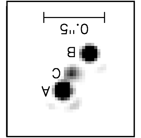
Figure 1: NICMOS image of APM08279+5255 showing the three lensed images of the QSO (adapted from Ibata et al. 1999). The F110W magnitudes of the three components are as follows: A = 13.45$\pm 0.02$, B = 13.74$\pm 0.02$, C = 15.37$\pm 0.03$ .

2 Observations

Observations with STIS on HST were obtained over the period November 2001–November 2002. Over a total of 25 orbits, we used five different settings of the G750M grating to obtain complete coverage over the wavelength region $\sim 6000-8600$ Å. With the 0.2 arcsec wide slit the dispersion is 0.55 Å pixel^-1 and the spectral resolution 1.6 Å FWHM (80 – 55 km s^-1). Table 1 summarises the observations. The acquisition was achieved by aligning the slit along the bright components A and B and then off-setting perpendicularly by 0.02  arcsec to centre on the faint, spatially intermediate image C. Between each exposure the targets were stepped along the slit by 1 arcsec.

In this paper, we also make use of the ground-based echelle spectrum of APM08279+5255 obtained with HIRES on the Keck I telescope (obtained in April and May 1998). A detailed description of those observations (and associated data reduction) can be found in Ellison et al. (1999a). In brief, we obtained a total of 8.75 hours of spectroscopy for APM08279+5255 with complete wavelength coverage between 4400 and 9250 Å. The spectral resolution of the data is 6 km s^-1 and the typical signal-to-noise ratio is S/N $\simeq 100$ per pixel. The three QSO images are spatially unresolved in these spectra. The data are publicly available via an ftp server at the Institute of Astronomy, Cambridge (ftp://ftp.ast.cam.ac.uk/pub/papers/APM08279).

3 Data Reduction

Figure 2: STIS spectra (arbitrary flux units) of the 3 LOS with the main absorption systems marked. Tick marks refer to systems listed in Table 2.

Figure 2: Contd.

Figure 2: Contd.

Figure 2: Contd.

Figure 2: Contd.

The STIS data were reduced as described by Lewis et al. (2002b). Despite the fact that the HIRES and STIS spectra were all mapped to a common vacuum heliocentric wavelength scale, we found that there remained some systematic velocity differences, internally between each of the three STIS spectra (for the three lines of sight), and also between the STIS and HIRES spectra. We suspect that this is caused by the slight offset from the centre of the slit of images A and B. The small shifts ($<20$ km s^-1) were corrected by performing a cross correlation between each STIS spectrum and the HIRES spectrum and applying the corresponding velocity adjustment. Note that this procedure, which corrects for the overall systematic offsets in the wavelength scales, should not affect the relative velocity shear of individual absorption systems.

Each STIS spectrum was normalised by fitting a cubic spline through a smoothed spectrum and using the HIRES spectrum as a guide to the continuum regions. This was particularly important in STIS settings where absorption lines are abundant, for example the $\lambda 6252$ setting. Equivalent widths for each absorption system were measured and errors estimated for counting statistics and continuum placement.

The final (un-normalised) extracted spectra are shown in Figure 2. The differences in broad emission line strengths have been previously pointed out by Lewis et al. (2002b) and are probably due to microlensing effects. Tick marks indicate the main absorption systems, and Table 2 identifies the species and redshifts. A total of 40 transitions identified from the HIRES spectrum were detected in the STIS data, including 10 Mg II systems (three of which are also detected in Fe II) and 16 C IV systems (five of which also exhibit Si IV absorption). We also detect Fe II and Al II in the DLA at $z_{\rm abs}=2.974$ and Ca II at $z_{\rm abs}=1.062$ in what is likely to be the lensing galaxy (Petitjean et al. 2000). There remain several unidentified lines in the HIRES spectrum (also present in the STIS data).

4 Equivalent Width Analysis

Due to the comparatively low resolution of the STIS spectra (FWHM $\simeq 55-80$ km s^-1), it is not possible to determine column densities directly by Voigt profile fitting of the absorption lines; thus we generally work here with the line equivalent widths.

We first examine the consistency between the STIS and HIRES measurements of equivalent width (EW). The fractional contribution to the total flux for the three components has been measured from NICMOS images to be 0.51$\pm 0.02$, 0.40$\pm 0.02$ and 0.09$\pm 0.03$ for A, B and C respectively (Ibata et al. 1999—see Figure 1). The corresponding fractional contributions to the EWs in the spatially unresolved HIRES spectrum can therefore be written as

$$EW_{HIRES}=0.51EW_{A}+0.40EW_{B}+0.09EW_{C}$$ (1)

Figure 3 shows the consistency check using equation (1). All of the lines are found to be in very good agreement, with the exception of two Mg II systems. System number 40 apparently shows some discrepancy between the ground-based and HST data. However, the HIRES spectrum is strongly affected by sky lines in this wavelength region and the system lies at the very limit of the STIS spectral coverage. The EW determinations consequently have unusually large errors (see Figure 2 and Table 2) and are actually only deviant at about the 1$\sigma$ level. The other anomaly is the case of Mg II $\lambda 2796$ at $z_{\rm abs}=1.813$ (number 37) which has similar values of EW in A and B, but is much weaker in C. In principle, such EW inconsistencies between the spatially resolved STIS spectra and the unresolved HIRES data may arise from a combination of QSO variability (Lewis, Robb & Ibata 1999) and time delays between the different LOS. However, there is no sign of EW variations between different epoch STIS data (taken a year apart), which is probably not surprising given the microlensing timescale is $\sim$ 40 years. Furthermore, other absorbers that do not fully cover all three sources do not show such deviations from the HIRES values. Since the other member of the Mg II doublet, $\lambda 2803$, and two Fe II transitions in the same absorption system (Fe II $\lambda 2600$ and $\lambda 1608$) all agree with the HIRES data, it is most likely that we have simply underestimated the measurement error for the stronger Mg II$\lambda$2796 line. Thus, overall, there is excellent agreement between the new data presented here and the earlier measurements by Ellison et al. (1999b).

Figure 3: Comparison of HIRES EWs and STIS EWs weighted by their respective flux contributions as given in equation 1. In all the figures in this paper, solid points indicate low ionization systems, such as Mg II and Fe II, as well as the DLA at $z_{\rm abs}=2.974$. Open points denote high ionization systems such as C IV and Si IV. Error bars are 1$\sigma$.

A straightforward conversion between equivalent width and column density is possible for unsaturated absorption systems located on the linear part of the curve of growth (i.e. for lines which are optically thin). Although we have the HIRES spectrum as a guide to which systems may be saturated, partial coverage effects may make strong lines appear unsaturated if they are only present in one or two of the LOS (or if they vary significantly between the LOS). In Figure 4 we plot the rest frame EWs of doublet components in the STIS data, multiplying the weaker component by 2 (to account for the lower value of the oscillator strength). For lines above $\sim$ 0.2 Å, we note the onset of a deviation from a one-to-one relation in some systems, indicative of possible saturation. Therefore, we adopt the conservative approach of only estimating column densities for absorbers with EW $<$ 0.2 Å. This method is vindicated by the very good agreement ($<<0.1$ dex) between the flux-weighted column densities from the STIS data (analogous to Figure 3 and Eqn. 1) and the Voigt profile fitted column densities of the HIRES data (e.g. Ellison et al. 2000).

Figure 4: Test for line saturation by comparing the rest frame EWs of doublet pairs of C IV and Mg II systems from the STIS spectra. On the $x$-axis we have plotted the value of equivalent width for the stronger component of each doublet, while on the $y$-axis we have plotted the EW of the weaker component multiplied by 2 to account for the lower value of oscillator strength. Deviation from a one-to-one relation above EW $\sim$ 0.2 Å indicates the onset of saturation for lines stronger than this limit.

5 Equivalent Width and Column Density Variations Between Sightlines

We now take advantage of the high spatial resolution of the STIS/HST combination to examine equivalent width differences between the sight-lines to the three images of APM08279+5255. We distinguish between high (e.g. C IV, Si IV) and low (e.g. Mg II, Fe II) ionization systems, since there is evidence that the characteristic scales of these absorbers are different (e.g. Rauch et al. 1999, 2002). Thus, in the plots that follow we use throughout solid symbols for low ionization systems and open symbols for high ionization systems. It is important to realise that, since the rest-frame wavelengths of the transitions of the high ions are generally lower than those of the low ions, the two sets of absorption lines probe quite different redshifts (and therefore transverse spatial scales) in the data analysed here. We also note that there are a number of high ionization transitions at redshifts $z_{\rm abs}\sim z_{\rm em}$ (e.g. absorber numbers 21, 23, 24 and 32–36 in Tables 2 and 3). In the following analysis we have not included absorption systems within 5000 km s^-1 of the QSO emission redshift because their locations along the lines of sight cannot be deduced if their redshifts are not cosmological. For absolute variations, we consider only systems with EW $<0.2$ Å in the stronger member of the doublet, so that we can convert to column density ($N$, measured in atoms cm^-2) assuming that the lines are on the linear part of the curve of growth, where

$$N=1.13\times 10^{20}\frac{EW(\rm\AA)}{\lambda_{0}^{2}f}$$ (2)

where $f$ is the oscillator strength and $\lambda_{0}$ is the rest wavelength of the transition in Å.

5.1 High Ionization Systems

Figure 5: Comparison of rest frame EWs between lines of sight A and B. Limits in this and all subsequent figures are 3$\sigma$.

Figure 6: As for Figure 5 but for LOS A and C.

We identify a total of 16 high ionization systems with LOS separations 0.028–0.340 $\leavevmode\nobreak\ h_{70}^{-1}$ kpc. This is an excellent complement at small scales to the study of high ionization systems by Rauch et al. (2001a) who probed scales up to 5 kpc but with only a few systems at separations less than 0.1 kpc. 

In Figures 5 and 6 we compare the equivalent widths between LOS A–B (largest separation) and A–C (smallest separation) respectively. In all cases the equivalent widths of high ionization systems show only mild differences between the different LOS, indicating that the structures which give rise to them are relatively uniform over scales of a few hundred pc. C IV equivalent width differences between sight-lines generally amount to less than 50 mÅ, which corresponds to column densities $\log N$(C IV)$<13.1$, see Figure 7. Figure 8 shows the fractional EW variation between sightlines as a function of LOS separation (all three A–B, B–C and A–C pairs are included). Typically the fractional equivalent width difference $\Delta EW=\frac{\mid\leavevmode\nobreak\ EW_{1}-EW_{2}\leavevmode\nobreak\ \mid}{max(EW_{1},EW_{2})}$ is less than 30%, although the errors can be large. There is no clear trend between variation and LOS separation on all scales below $\sim 0.4$ kpc. Presumably the suggestion of a possible decrease in $\Delta$ EW for LOS $<0.1$ kpc in the data by Rauch et al. (2001a) was an artifact of small number statistics, since we see no evidence of it in the more extensive set of measurements presented here (although see below and Figure 11).

So far we have considered only whole absorption systems, without reference to their multi-component structure. While we do see hints of variations on a component-by-component basis even with our (limited) spectral resolution (one example is system 12—see Figure 2), we will investigate such differences in more detail in a future paper by reconstructing the high resolution line profiles (Aracil et al., in preparation).

Figure 7: Absolute column density differences for high ionization systems as a function of proper LOS separation

Figure 8: Fractional EW differences for high ionization systems as a function of proper LOS separation

5.2 Low Ionization Systems

We identify a total of 17 low ionization systems (mostly Mg II and Fe II) with LOS separations 0.41–3.09 $\leavevmode\nobreak\ h_{70}^{-1}$ kpc. This list includes Fe II $\lambda 1608$ and Al II $\lambda 1670$ associated with the DLA at $z_{\rm abs}=2.974$ previously studied by Petitjean et al. (2000). As can be appreciated from inspection of Figures 5 and 6, there can be significant LOS differences in the absorption lines from low ionization gas, with several instances where absorption is detected in only one or two of the three sight-lines .

Figure 9: Absolute column density differences for low ionization systems as a function of proper LOS separation

Figure 10: Fractional EW differences for low ionization systems as a function of proper LOS separation

In Figures 9 and 10 we show the absolute and fractional variations between sightlines as a function of LOS separation. This is the first time that the sizes of low ionization systems have been studied in relatively large numbers, due to the particularly rich spectrum and the triple nature of APM08279+5255. We find that the low ionization systems can have much larger fractional variations than the high ionization systems for LOS separations $>0.5$ $\leavevmode\nobreak\ h_{70}^{-1}$ kpc, with several cases where $\Delta EW>80$%. However, some systems exhibit little variation, even over 1 $\leavevmode\nobreak\ h_{70}^{-1}$ kpc or more. Since Rauch et al. (2002) found that individual low ionization clouds can rarely be traced over more than a few hundred pc, this is likely an effect of the combined variation of several clouds. Again, our inversion analysis which will be presented in Aracil et al. will investigate this in more detail.

Kobayashi et al (2002) have detected structural LOS differences in the Mg II line of the $z_{\rm abs}$=2.974 DLA from ground based IR spectra taken in good seeing conditions. This structure is also apparent in our lower resolution spectra; the Al II $\lambda$1670 transition is narrower in LOS B than A and C (although the Fe II absorption is too weak to discern such differences). However, the absolute difference in EW between the LOS is small, and consistent with those seen in other (non-damped) low ionization systems at small separations.

In Figure 11 we summarise the fractional variations (based either on column density or EW, as published) in high and low ionization systems by combining measurements made here with those available in the literature (Lopez et al. 2000; Rauch et al. 2001a; Rauch et al. 2002; Churchill et al. 2003). All the literature values have been converted to the cosmology adopted in the present paper. We plot the mean fractional variation for each separation and the scatter (standard deviation) for that bin. The upper limits obtained from APM08279+5255 (e.g. Figure 10) have been treated as detections, with the effect that the scatter is slightly reduced. However, literature upper limits could only be included when a detection limit was quoted. It can be seen that for the low ionization systems the mean variation is the same for all separations within the large scatter. This is probably due to the fact that individual components cannot be traced over more than a few hundred pc. The high ionization systems, however, show a clear trend for larger variations with increasing LOS separation. The scatter is relatively small compared with the low ionization systems, except for the 0.5 – 1.0 kpc bin which only contains two data points.

Figure 11: Fractional EW variations for low and high ionization systems from this work and the literature (Lopez et al. 2000; Rauch et al. 2001a; Rauch et al 2002; Churchill et al 2003). We only include values based on Mg II, Fe II, Si IV and C IV to be consistent with measurements towards APM08279+5255.

6 Coherence Scales of Absorption Systems

6.1 High Ionization Systems

Since all of the high ionization systems detected in the present dataset are common to all three LOS, we can only place a lower limit on the size of the absorbers of $\sim$ 0.3 $\leavevmode\nobreak\ h_{70}^{-1}$ kpc (this being the largest beam separation in Table 2). This limit is not very instructive given that observations of wider QSO pairs have established much larger coherence lengths for C IV systems (e.g. Petitjean et al. 1998; Lopez et al. 2000). More recently, Tzanavaris & Carswell (2003) concluded that that the most probable size for individual components of C IV complexes is $\sim 3\,h_{70}^{-1}$ kpc, if the ‘clouds’ have a spherical geometry.

6.2 Low Ionization Systems

Since we have a modest number of low ionization systems, several of which are only seen in 1 or 2 of the LOS, we can employ a maximum likelihood analysis to estimate the coherence scale of the structures producing them based on LOS coincidences and anti-coincidences. This analysis relies on at least one anti-coincidence, otherwise the likelihood function is a monotonically increasing function of cloud radius. Similar analyses have been performed previously for Ly$\alpha$ forest clouds and C IV systems, but this is the first such determination for low ionization gas halos.

We adopt the formalism of McGill (1990) with the modification by Dinshaw et al. (1997). One ingredient in this analysis is the assumed geometry of the absorber, uniform spheres or flattened, randomly inclined, disks being the two usual approximations. There is evidence that rotation in the plane of the stellar disk of Mg II galaxies is reflected in the absorption gas kinematics in at least some cases (Steidel et al. 2002), although absorption and emission kinematics are not always well correlated (Lanzetta et al. 1997; Ellison, Mallen-Ornelas & Sawicki 2003). More generally, the success of a simple Holmberg relation in describing the incidence of Mg II absorption shows that a spherical gas distribution is a good approximation (Steidel 1995), and this is the model we adopt here. For pairs of LOS intersecting spherical clouds, the probability that a halo is intersected by the second LOS, given that it is seen in the first, is given by

$$\phi(X)=\frac{2}{\pi}\left\{\arccos\left[X(z)\right]-X(z)\sqrt{1-X(z)^{2}}\right\}$$ (3)

for $0\leq X(z)\leq 1$ and zero otherwise. Here, $X(z)=S(z)/2R$ where $S(z)$ is the LOS separation and $R$ is the absorber coherence radius. This of course assumes that all absorbers are of the same size and that there is no column density variation within a ‘cloud’. In order to make maximum use of the information available we actually want to calculate the probability that both LOS are intersected, if $either$ LOS shows absorption. That is, we consider anti-coincidences in any combination of A, B and C. This probability is given by

$$\psi=\frac{\phi}{2-\phi}$$ (4)

And the likelihood function as a function of coherence radius is given by

$${\cal L}(R)=\prod_{i}\psi\left[X(z_{i})\right]\prod_{j}\left\{1-\psi\left[X(z_{j})\right]\right\},$$ (5)

where $i$ and $j$ denote the number of coincidences and anti-coincidences. We note that although the original formulism of McGill (1990) was designed for pairs of sightlines, we can still use combinations of A, B and C to investigate the coherence scale of Mg II absorption, rather than the sizes of individual components. Figure 12 shows the results of our maximum likelihood analysis. For the whole sample of Mg II systems in APM08279+5255 (16 pairs of LOS coincidences and 13 anti-coincidences), we find that the most probable value for the absorber coherence scale is $R=3.0\,h_{70}^{-1}$ kpc, with 95% confidence limits of 2.1 and 6.2 kpc. Similarly small sizes for Mg II systems have been previously inferred from partial coverage arguments by Petitjean et al. (2000). This coherence scale contrasts with the much smaller sizes inferred for individual components (Churchill et al. 2003; Rauch et al. 2002). However, the value $R=3.0\,h_{70}^{-1}$ kpc is about one order of magnitude smaller than the dimensions of Mg II absorbing halos deduced from (a) the number density of absorbers per unit redshift and (b) the impact parameters from the QSO of the galaxies producing the absorption, in cases where they have been identified (Bergeron & Boissé 1991; Steidel 1993; Steidel, Dickinson, & Persson 1994). Previous analyses of Mg II absorbers in lensed sightlines have also inferred scales of several tens of kpc (Smette et al 1995).

The answer to this apparent discrepancy may lie in the fact that most statistical samples of Mg II absorbers have considered strong lines, with rest-frame equivalent widths greater than 0.3 Å, whereas many of the systems analysed here are ‘weak’ absorbers (Churchill et al 1999; Rigby, Charlton & Churchill 2002). If we consider separately the strong systems (all LOS exhibiting EW$\geq 0.3$ Å), the maximum likelihood analysis does not converge because there are no anti-coincidences in our sample, so that we can only infer a lower limit to the radius/coherence scale, $R>1.4\,h_{70}^{-1}$ kpc (from the largest LOS separations sampled here). This is also consistent with the larger sizes of strong Mg II systems inferred by Smette et al (1995). For the remainder of the ‘weak’ systems the maximum likelihood analysis (with 8 coincidences and 13 anti-coincidences) yields a most probable radius of $2.0\,h_{70}^{-1}$ kpc with 95% confidence limits of 1.5 and 4.4 kpc (see Figure 12). If the adopted lens redshift is in fact $z_{lens}<1.062$ this would imply even smaller beam separations (e.g. by $\sim$50% for $z_{lens}=0.6$), so our conclusion that weak absorbers have small sizes would remain unchanged.

For the DLA at $z_{\rm abs}=2.974$, where all absorption lines are seen in all three sight-lines, we similarly deduce a lower limit to the size of 0.34 $\leavevmode\nobreak\ h_{70}^{-1}$ kpc. This is in agreement with the size deduced by Petitjean et al. (2000) based on the absence of partial coverage in the Ly$\alpha$ absorption line.

Figure 12: Maximum likelihood distribution (thin solid line) and cumulative distribution (dashed line) for spherical halos normalized to the peak value. The most likely coherence radius is found to be R=3.0 $\leavevmode\nobreak\ h_{70}^{-1}$ kpc with 95 % confidence limits of 2.1 and 6.2 $\leavevmode\nobreak\ h_{70}^{-1}$ kpc. The bold lines show the results obtained if we restrict ourselves to weak (EW$<$0.3 Å) Mg II systems only, for which we deduce a most likely scale of $R$=2.0 $\leavevmode\nobreak\ h_{70}^{-1}$ kpc with 95% confidence limits of 1.5 and 4.4 $\leavevmode\nobreak\ h_{70}^{-1}$ kpc.

7 Velocity Shear

Figure 13: Consistency check for cross-correlation shear velocities. We compare the difference between the cross correlation velocities for $v_{A}-v_{B}$ and $v_{B}-v_{C}$ with that computed for $v_{B}-v_{C}$.

Velocity shear between sightlines was calculated by cross-correlating the absorption line profiles for each LOS combination using the task fxcor in IRAF. Errors within this package are calculated using the formalism of Tonry & Davis (1979). An independent error check can be carried out using the fact that shifts between each LOS combination form a closed system. That is, the difference in the calculated shifts between A–B and A–C should equal the shift between C–B. We plot the results of this consistency check in Figure 13. It can be seen that in most cases the agreement is very good, and well within the formal error bars.

7.1 High Ionization Systems

Figure 14: Velocity shear as a function of separation for high ionization systems.

In Figure 14 we present the shear velocities as a function of LOS separation for high ionization systems. We find that the shear is generally less than 20 km s^-1 for separations up to $\sim$0.35 $\leavevmode\nobreak\ h_{70}^{-1}$ kpc. Again, this complements the results by Rauch et al (2001a) who had few points below 0.2 kpc. With these additional points at small separations, it can now be seen that shear velocities in high ionization systems are generally less than 15–20 km s^-1 at separations smaller than 0.5 $\leavevmode\nobreak\ h_{70}^{-1}$ kpc, with evidence for an increase in shear at larger separations (Rauch et al. 2001a).

7.2 Low Ionization Systems

Figure 15: Velocity shear as a function of separation for low ionization systems.

The velocity shear for low ionization systems is shown in Figure 15. We do not find any evidence for the significant increase in shear on scales greater than 1 kpc seen in C IV systems by Rauch et al. (2001a). The observed shear between the metal lines of the DLA is also small, less than 10 km s^-1, consistent with the those of the other, weaker, low ionization absorbers. However, our analysis is limited by the fact that we have insufficient spectral resolution to perform a column density weighted calculation (c.f. Rauch et al. 2002; Churchill et al. 2003). This is particularly important for the low ionization systems where the scale of individual components is much smaller than our proper beam separation. This is highlighted by the Mg II system at $z=1.813$ where the absorption lines are of of similar strengths in LOS A and B, but are much weaker in the spatially intermediate LOS C. Our cross-correlation velocity shear therefore traces the shift between the strongest components in each LOS.

8 Chemical Uniformity

In cases where two ions are observed in more than one LOS (and the lines have EW$<$0.2 Å so as to permit a column density determination), we can test for transverse variations in the ratio of their column densities. Such variations may result from differences between the sightlines in chemical composition, dust depletion and ionization conditions, or any combination of these. However, since we typically only observe two elements in each absorption system, we do not have sufficient information to disentangle these effects.

There are two high ionization systems for which we can study transverse abundance differences through the C IV/Si IV ratio. Table 4 summarises these results; relative column densities for weak high ionization systems agree to within 0.1 dex over a few hundred pc. Since we have found that high ionization systems vary little between LOS, it is not surprising that their column density ratios are in good agreement too. Unfortunately, we can not investigate differences in the low ionization systems (apart from the DLA) since all the Mg II systems which have associated Fe II are too strong to determine accurate column densities.

For the DLA (or possible sub-DLA), we have available low ionization lines of Al II and Fe II. Although Al II $\lambda$1670 is usually saturated in DLAs, we see no evidence for this in the HIRES spectrum and the lack of flat-bottomed profiles argues against de-saturation by partial coverage. This is not unexpected given the relatively low $N$(HI) of this DLA (Petitjean et al 2000). Since Al II and Fe II represent the major ionisation stages of these elements in DLAs (and ionisation corrections are relatively small even for sub-DLAs, see Dessauges-Zavadsky et al. 2003), we can use the EWs in Table 3 to deduce abundance ratios [Al/Fe] $=+0.15^{+0.09}_{-0.12}$, $-0.04^{+0.09}_{-0.13}$, $+0.05^{+0.15}_{-0.22}$ in A, B and C respectively. Although these values may suggest mild variations of the [Al/Fe] ratio between the three sight-lines, they are actually all consistent with the solar value within the errors . Chemical uniformity in absorbers has been previously pointed out both along (Prochaska 2003) and across (Churchill et al. 2003) quasar lines of sight. Our observations concur with these findings, with little detected variation over $\sim$ 350 pc.

9 Discussion

In the Milky Way, the warm, highly ionized gas component is relatively smoothly distributed with little or no change in column density over several degrees on the sky; SiIV and CIV absorptions in particular are generally well matched (Savage, Sembach & Lu 1997). In contrast, very small-scale variations (on the order of a few AUs) have been observed in the cold ($\sim$ 100 K) neutral gas component (traced by Na I) of the interstellar medium (e.g. Andrews, Meyer & Lauroesch 2001; Lauroesch, Meyer & Blades 2000). The singly ionized species of Fe II and Mg II studied here are intermediate between these two phases and most likely occur in a warm neutral medium. These species trace each other well in terms of velocity structure, as well as showing a close kinematic relation to Ca II which is more often studied in the local ISM (e.g. Welty, Morton & Hobbs 1996; Redfield & Linsky 2002). Such low ionization species do exhibit some variation on scales of a few tens to tens of thousands of AU, but the LOS differences are less marked than in the cold phase traced by Na I (e.g. Meyer & Roth 1991; Meyer & Blades 1996; Lauroesch et al 1998; Price, Crawford & Howarth 2001). Variation in Ca II and other low ions can be seen both in terms of velocity structure and column density, although such variation is by no means ubiquitous (e.g. Rauch et al. 2002). The presence of these small scale variations can be explained by density contrast within a diffuse cloud where the bulk of the low ionization gas is concentrated in the highest density peaks (Lauroesch & Meyer 2003). The variation of different species between lines of sight (or temporally in a single Galactic sightline) is therefore dependent not only on the size of the ‘cloud’ itself, but also on the local physical conditions that maintain the ionization balance.

Qualitatively similar trends have been observed in high redshift absorbers. On scales of a few pc the high ionization gas is effectively featureless (Rauch et al. 1999), with variations typically $<$30% for transverse separations of 50 pc – 5 $\leavevmode\nobreak\ h_{70}^{-1}$ kpc (Rauch et al. 2001a; this work). However, the location of this high ionization gas remains uncertain. The ubiquity of C IV absorption associated with the Ly$\alpha$ forest, even at low H I column densities (e.g. Ellison et al. 2001), and coherence lengths of more than 100 $\leavevmode\nobreak\ h_{70}^{-1}$ kpc (Petitjean et al 1998; Lopez, Hagen & Reimers 2000) suggest an intergalactic origin. However, Adelberger et al. (2003) find a strong correlation between Lyman break galaxies and C IV absorption out to impact parameters of hundreds of kpc, indicating a link between galaxy winds and metal enriched gas. A similar conclusion was reached by Rauch et al. (2001a) based on the small internal turbulence of C IV systems.

Similar to the situation in Galactic sightlines, high redshift absorbers exhibit much stronger variation in the low ionization species. Given the pervasive small-scale structure observed in the Milky Way, it is not surprising that individual Mg II components cannot be traced between sight-lines separated by a few tens to a few hundred pc (Rauch et al. 1999, 2002) and that large fractional EW differences are common in these systems (this work). However, coincidences of absorption between LOS indicate that there is coherence in the absorption structure on somewhat larger scales. This can be compared with the ‘clumpy but coherent’ structure seen in Mg II and other low ions in the local ISM out to at least 100 pc (Redfield & Linksy 2002). Based on a maximum likelihood analysis, we have been able to infer the likely coherence length of weak Mg II systems (as opposed to the size of individual components) $R\sim 2$ $\leavevmode\nobreak\ h_{70}^{-1}$ kpc. This coherence scale must be understood in context with the overall galaxy sizes inferred for strong Mg II systems (e.g. Steidel 1995) which show absorption out to several tens of kpc from the absorbing galaxies.

One possibility is that the weak absorbers represent a distinct population whose actual sizes are a few kpc, comparable to those of present-day dwarf galaxies. Compared with strong Mg II absorbers, the weak systems in our sample have relatively simple kinematic structure and are spread over narrow velocity ranges. In generic cold dark matter models of galaxy formation (e.g. Mo & Miralda-Escude 1996) there is a steep correlation between circular velocity and halo dimension which agrees with the small sizes derived from our maximum likelihood analysis. However, the small sizes inferred here contradict the suggestion by Churchill & Le Brun (1998) that weak Mg II absorbers are ‘giant’ LSB systems, although low luminosities remain highly feasible.

Alternatively, the weak Mg II systems may occur in sightlines through large galaxies, but in regions where interstellar clouds have lower filling factors leading to smaller inferred coherence lengths. Indeed, Rigby et al. (2002) suggest that although single cloud weak Mg II systems (see below) may arise from a distinct population, the multi-component systems are likely have the same origin as the strong clouds. In this picture, the absorbing clouds are made up of pc-scale components with a total covering factor of about unity (Srianand & Khare 1994; Rauch et al 2002) in the central few tens of kpc of the galaxy. Further out, the filling factor is smaller, so that anti-coincidences may be observed indicating smaller sizes. Inferred scales of $2R\sim$ 4 $\leavevmode\nobreak\ h_{70}^{-1}$ kpc compared to $\sim$ 40 kpc (Steidel 1995) would imply filling factors that are an order of magnitude smaller for the weak Mg II systems. Smaller filling factors would also explain the tendency towards fewer components in low EW systems. The above scenario is qualitatively born out by an observed anti-correlation between Mg II column density and galaxy impact parameter (Churchill et al. 2000). Indeed, Churchill et al. (2000) find that all high impact parameter intersections have small EW Mg II absorbers. This scenario could be tested with an imaging and spectroscopic campaign to identify the galaxies responsible for absorption.

Finally, we comment on the observation that two thirds of weak Mg II absorbers have been previously found to be single cloud systems (Rigby et al. 2002). The HIRES spectra of APM08279+5255 (Ellison et al. 1999b) show this not to be the case here; all of the eight weak Mg II systems we have identified exhibit multiple velocity components when observed with HIRES. Bearing in mind that the HIRES observations do not resolve the three images, this multicomponent structure is probably a reflection of the small scale variations seen by Rauch et al. (2002). Moreover, the exceptional S/N of the HIRES spectrum of APM08279+5255 reveals components that would not normally be identified in most spectra. The Mg II system at $z_{\rm abs}$=1.291, which has an unresolved main component and a weaker, broader feature $\sim$ 25 km s^-1 away (Ellison et al. 1999b), would have been classified by Rigby et al. (2002) as a single cloud weak absorber in a lower S/N spectrum. Using ionization models, Rigby et al. found the sizes of single cloud absorbers with Fe II to be $\sim 10$ pc. The models for weak Mg II systems without Fe II are less well constrained, allowing for cloud sizes which vary between a few pc and several tens of kpc. Since the system at $z_{\rm abs}$=1.291 would have been classified as an (albeit, Fe II free) weak single cloud absorber in spectra of S/N typical of the data used by Rigby et al., we can now significantly improve upon the size estimate of this type of absorber with the STIS data. Given that absorption is detected in both LOS A and B (in C the S/N is insufficient to provide useful information) we deduce a minimum size of 2.4 $h_{70}^{-1}$ kpc, more than 20 times larger than the value estimated (indirectly) for the Fe-rich systems.

10 Conclusions

In this paper, we have presented moderate resolution STIS spectra of the tripled imaged QSO APM08279+5255, and focussed our analysis on an investigation of the sizes and coarse structure of intervening metal absorption systems. By capitalising upon the unusually absorption-rich lines of sight offered by the triply imaged QSO APM08279+5255, we have significantly increased the number of high ionization systems (primarily C IV) probed at small ($<0.1$ $\leavevmode\nobreak\ h_{70}^{-1}$ kpc) separations. This study is also the most comprehensive to date of the variation of low ionization (e.g. Mg II) systems. Our principal conclusions are as follows.

1. High ionization systems generally show small EW variations on scales of a few tens to a few hundreds of pc, although we find evidence in at least one system for small component differences across the LOS. This complements the work of Rauch et al. (2001a) whose observations probed mostly larger separations for C IV systems in three pairs of lensed QSOs. Taken together, all of these data indicate a steady increase in fractional variation with increasing LOS separation, although rarely exceeding 40%. All the high ionization systems occur in all three lines-of-sight to APM08279+5255, implying sizes of $>3$ $\leavevmode\nobreak\ h_{70}^{-1}$ kpc.

2. In contrast to the high ionization systems, low ionization complexes exhibit significant variation ($\Delta$ EW $>80$%) on scales greater than a few hundred pc, although we lack the spectral resolution to trace individual clouds between sightlines. There is no trend of fractional variation as a function of LOS separation, which can be explained by the small sizes ($<$ few hundred pc) of individual components. For strong (EW$>$ 0.3 Å) Mg II systems we can only infer a minimum radius of $\sim$ 3 $\leavevmode\nobreak\ h_{70}^{-1}$ kpc, although the actual size is likely to be significantly larger (Steidel 1995; Smette et al 1995). For weaker systems (EW$<$ 0.3 Å), we apply a maximum likelihood method and infer a most probable coherence scale of 2.0 $h_{70}^{-1}$ kpc with 95% confidence limits of 1.5 and 4.4 kpc. Therefore, we suggest that these are either a population distinct from strong Mg II systems, perhaps associated with dwarf galaxies, or that they occur in the outer regions of large, luminous galaxies where their filling factor is lower.

3. The velocity shear for both high and low ionization systems is small, typically less than 20 km s^-1. However, since we can not trace individual low ionization components, the shear velocities for these systems reflects mainly the shift in the location of the strongest component(s).

4. For two of the high ionization systems where the lines are opticall thin and the EWs can be converted to column densities, we find consistent ratios of $N$(C IV)/$N$(Si IV) between LOS. The abundance ratio of [Al/Fe] in the DLA (or possible sub-DLA) also exhibits only mild variation ($<0.1$ dex) and is approximately solar in the three LOS.

5. We note a deficit of single cloud weak Mg II absorbers in the HIRES spectrum of APM08279+5255 and speculate that this may be due to the superposition of sightlines in the spatially unresolved ground-based data. This and other issues will be addressed in a future paper (Aracil et al, in preparation) that uses an inversion analysis to produce high spectral resolution for each LOS by combining information from the STIS and HIRES spectra.

$\lambda_{0}$	Range(Å)	Date	Total Exp Time(s)	S/N
				LOS A	LOS B	LOS C
6252	5970–6530	Nov 10 2001	14 900	60	45	25
6768	6490–7050	Dec 26 2001	11 800	60	45	25
7283	7000–7560	Dec 26-27 2001	11 800	60	40	25
7795	7500–8070	Dec 27 2001, Nov 25 2002	14 900	40	35	20
8311	8030–8600	Nov 25-26 2002	21 100	30	25	17

Table 1: Log of STIS Observations

Absorber No.	Transition	Redshift	A-B linear	A-C linear
			sepn (kpc h${}_{70}^{-1}$)	sepn (kpc h${}_{70}^{-1}$)
1	Mg II $\lambda\lambda$2796, 2803	1.181	2.702	1.067
2	Si IV $\lambda\lambda$1393, 1402	3.379	0.164	0.065
3	C IV $\lambda\lambda$1548, 1550	2.974	0.340	0.134
4	Mg II $\lambda\lambda$2796, 2803	1.209	2.620	1.034
5	Mg II $\lambda\lambda$2796, 2803	1.211	2.614	1.032
6	Si IV $\lambda\lambda$1393, 1402	3.502	0.120	0.047
7	Si IV $\lambda\lambda$1393, 1402	3.514	0.116	0.046
8	C IV $\lambda\lambda$1548, 1550	3.109	0.275	0.109
9	Fe II $\lambda$1608	2.974	0.340	0.134
10	C IV $\lambda\lambda$1548, 1550	3.134	0.264	0.104
11	Mg II $\lambda\lambda$2796, 2803	1.291	2.395	0.945
12	C IV $\lambda\lambda$1548, 1550	3.171	0.247	0.098
13	C IV $\lambda\lambda$1548, 1550	3.203	0.233	0.092
14	C IV $\lambda\lambda$1548, 1550	3.239	0.219	0.086
15	Fe II $\lambda$1608	1.550	1.811	0.715
16	Fe II $\lambda$1608	1.552	1.807	0.713
17	Al II $\lambda$1670	2.974	0.340	0.134
18	Fe II $\lambda$1608	1.813	1.368	0.540
19	C IV $\lambda\lambda$1548, 1550	3.379	0.164	0.065
20	C IV $\lambda\lambda$1548, 1550	3.386	0.161	0.064
21	Si IV $\lambda\lambda$1393, 1402	3.893	0.005	0.002
22	Mg II $\lambda\lambda$2796, 2803	1.444	2.029	0.801
23	Si IV $\lambda\lambda$1393, 1402	3.913	…	…
24	Si IV $\lambda\lambda$1393, 1402	3.917	…	…
25	C IV $\lambda\lambda$1548, 1550	3.502	0.120	0.047
26	C IV $\lambda\lambda$1548, 1550	3.514	0.116	0.046
27	C IV $\lambda\lambda$1548, 1550	3.558	0.101	0.040
28	Mg II $\lambda\lambda$2796, 2803	1.550	1.811	0.715
29	Mg II $\lambda\lambda$2796, 2803	1.552	1.807	0.713
30	C IV $\lambda\lambda$1548, 1550	3.655	0.071	0.028
31	Fe II $\lambda$2600	1.813	1.368	0.540
32	C IV $\lambda\lambda$1548, 1550	3.857	0.014	0.005
33	C IV $\lambda\lambda$1548, 1550	3.893	0.005	0.002
34	C IV $\lambda\lambda$1548, 1550	3.899	0.003	0.001
35	C IV $\lambda\lambda$1548, 1550	3.912	…	…
36	C IV $\lambda\lambda$1548, 1550	3.917	…	…
37	Mg II $\lambda\lambda$2796, 2803	1.813	1.368	0.540
38	Ca II $\lambda\lambda$3934, 3969	1.062	3.086	1.218
39	Mg II $\lambda\lambda$2796, 2803	2.042	1.070	0.422
40	Mg II $\lambda\lambda$2796, 2803	2.067	1.041	0.411

Table 2: A list of intervening Mg II, C IV and Si IV absorbers. Proper linear separations in are calculated assuming the lens at $z$=1.06, A–C separation = 0.15 arcsec, A–B separation = 0.38 arcsec with $\Omega_{M}$=0.3, $\Omega_{\Lambda}$=0.7. The transition numbers refer to tick marks in Figure 2.

No.	Absorber	Redshift	LOS A		LOS B		LOS C		HIRES
			EW1	EW2	EW1	EW2	EW1	EW2	EW1	EW2
1	MgII	1.181	2.57$\pm$0.04	2.26$\pm$0.02	3.03$\pm$0.04	2.98$\pm$0.02	2.88$\pm$0.04	2.68$\pm$0.02	2.595	2.433
2	SiIV	3.379	…	0.08$\pm$0.02	…	0.09$\pm$0.02	…	0.09$\pm$0.02	…	0.095
3	CIV	2.974	0.17$\pm$0.01	0.10$\pm$0.01	0.17$\pm$0.02	0.08$\pm$0.01	0.17$\pm$0.03	0.06$\pm$0.02	0.167	0.076
4	MgII	1.209	0.05$\pm$0.01	0.03$\pm$0.01	0.06$\pm$0.02	0.04$\pm$0.02	$<$0.03	$<$0.03	0.051	0.034
5	MgII	1.211	0.37$\pm$0.01	0.34$\pm$0.01	$<$0.03	$<$0.03	0.16$\pm$0.04	0.25$\pm$0.04	0.234	0.236
6	SiIV	3.502	0.14$\pm$0.01	0.09$\pm$0.01	0.18$\pm$0.01	0.09$\pm$0.01	0.14$\pm$0.02	0.08$\pm$0.02	0.145	0.087
7	SiIV	3.514	0.04$\pm$0.01	0.03$\pm$0.01	0.05$\pm$0.01	0.02$\pm$0.01	0.06$\pm$0.02	$<$0.03	0.043	0.018
8	CIV	3.109	0.31$\pm$0.01	0.18$\pm$0.01	0.28$\pm$0.01	0.15$\pm$0.01	0.30$\pm$0.02	0.13$\pm$0.02	0.308	0.175
9	FeII	2.974	0.04$\pm$0.01	…	0.05$\pm$0.01	…	0.05$\pm$0.02	…	0.041	…
10	CIV	3.134	0.14$\pm$0.01	0.08$\pm$0.01	0.16$\pm$0.02	0.12$\pm$0.01	0.17$\pm$0.03	0.11$\pm$0.03	0.143	0.080
11	MgII	1.291	0.08$\pm$0.01	0.05$\pm$0.01	0.03$\pm$0.01	$<$0.03	$<$0.03	$<$0.03	0.046	0.028
12	CIV	3.171	0.26$\pm$0.01	0.13$\pm$0.01	0.22$\pm$0.02	0.08$\pm$0.02	0.32$\pm$0.03	0.15$\pm$0.03	0.242	0.131
13	CIV	3.204	…	0.09$\pm$0.01	…	0.10$\pm$0.02	…	0.10$\pm$0.03	…	0.098
14	CIV	3.239	0.04$\pm$0.01	0.03$\pm$0.01	0.05$\pm$0.01	0.02$\pm$0.01	0.07$\pm$0.02	$<$0.03	0.051	0.027
15	FeII	1.550	0.10$\pm$0.02	…	$<$0.02	…	0.09$\pm$0.03	…	…	…
16	FeII	1.552	0.08$\pm$0.01	…	$<$0.02	…	$<$0.03	…	0.041	…
17	AlII	2.974	0.19$\pm$0.01	…	0.14$\pm$0.01	…	0.20$\pm$0.03	…	0.202	…
18	FeII	1.813	0.18$\pm$0.01	…	0.21$\pm$0.02	…	0.03$\pm$0.03	…	…	…
19	CIV	3.379	0.37$\pm$0.02	…	0.33$\pm$0.02	…	0.32$\pm$0.03	…	0.352	…
20	CIV	3.386	…	0.11$\pm$0.02	…	0.12$\pm$0.02	…	0.10$\pm$0.02	…	0.120
21	SiIV	3.893	0.35$\pm$0.01	0.28$\pm$0.01	0.36$\pm$0.01	0.28$\pm$0.01	0.34$\pm$0.02	0.28$\pm$0.02	0.364	0.284
22	MgII	1.444	0.04$\pm$0.01	…	0.04$\pm$0.01	…	$<$0.03	…	0.045	…
23	SiIV	3.913	0.33$\pm$0.01	0.20$\pm$0.01	0.32$\pm$0.01	0.21$\pm$0.01	0.26$\pm$0.02	0.27$\pm$0.02	…	…
24	SiIV	3.917	…	0.02$\pm$0.01	…	0.02$\pm$0.01	…	0.04$\pm$0.02	…	…
25	CIV	3.502	0.10$\pm$0.01	…	0.13$\pm$0.01	…	0.13$\pm$0.03	…	0.113	…
26	CIV	3.514	0.03$\pm$0.01	0.01$\pm$0.01	0.05$\pm$0.01	0.03$\pm$0.01	0.05$\pm$0.02	$<$0.03	0.043	0.028
27	CIV	3.558	0.05$\pm$0.01	0.02$\pm$0.01	0.04$\pm$0.01	0.03$\pm$0.01	0.04$\pm$0.02	$<$0.03	0.040	0.026
28	MgII	1.550	0.31$\pm$0.01	0.24$\pm$0.01	$<$0.02	$<$0.02	0.29$\pm$0.03	0.28$\pm$0.03	0.229	0.151
29	MgII	1.552	0.24$\pm$0.01	0.20$\pm$0.01	$<$0.02	$<$0.02	$<$0.03	$<$0.03	0.119	0.102
30	CIV	3.655	0.06$\pm$0.01	0.03$\pm$0.01	0.07$\pm$0.02	0.03$\pm$0.02	0.06$\pm$0.01	0.03$\pm$0.01	0.061	0.034
31	FeII	1.813	0.14$\pm$0.01	…	0.15$\pm$0.02	…	0.06$\pm$0.02	…	0.107	…
32	CIV	3.857	0.20$\pm$0.01	0.11$\pm$0.01	0.19$\pm$0.02	0.09$\pm$0.02	0.23$\pm$0.02	0.11$\pm$0.02	0.217	0.106
33	CIV	3.893	0.66$\pm$0.05	…	0.64$\pm$0.05	…	0.65$\pm$0.05	…	0.664	…
34	CIV	3.899	…	0.70$\pm$0.04	…	0.66$\pm$0.04	…	0.70$\pm$0.05	…	…
35	CIV	3.912	0.63$\pm$0.03	0.40$\pm$0.03	0.59$\pm$0.03	0.36$\pm$0.03	0.65$\pm$0.05	0.39$\pm$0.04	…	…
36	CIV	3.917	0.49$\pm$0.03	0.41$\pm$0.03	0.43$\pm$0.03	0.34$\pm$0.03	0.50$\pm$0.03	0.36$\pm$0.03	…	…
37	MgII	1.813	0.80$\pm$0.02	0.58$\pm$0.02	0.77$\pm$0.02	0.48$\pm$0.02	0.44$\pm$0.03	0.21$\pm$0.03	0.686	0.477
38	CaII	1.062	…	…	…	…	…	…	…	…
39	MgII	2.041	0.21$\pm$0.02	0.14$\pm$0.02	0.24$\pm$0.02	0.13$\pm$0.02	0.22$\pm$0.03	0.18$\pm$0.03	0.222	0.154
40	MgII	2.066	0.31$\pm$0.04	…	0.45$\pm$0.04	…	0.38$\pm$0.04	…	0.297	…

Table 3: Rest frame EW measurements (values for doublet components indicated by subscripts 1 and 2) for STIS and HIRES spectra. Upper limits are 3 $\sigma$. No data (‘…’) is given if the line is known from the HIRES spectrum to be contaminated or blended, or the line is not a multiplet.

Redshift	LOS A ratio	LOS B ratio	LOS C ratio
3.502	0.22$\pm$0.06	0.18$\pm$0.06	0.29$\pm$0.14
3.514	0.27$\pm$0.13	0.33$\pm$0.16	0.21$\pm$0.17

Table 4: Log N(C IV)/log N(Si IV) column density ratios for systems with EW$<$0.2 Å for each line of sight.