Molecular Hydrogen Emission Lines in Far Ultraviolet Spectroscopic Explorer Observations of Mira B

Abstract

We present new Far Ultraviolet Spectroscopic Explorer (FUSE) observations of Mira A’s wind-accreting companion star, Mira B. We find that the strongest lines in the FUSE spectrum are H₂ lines fluoresced by H I Ly$\alpha$. A previously analyzed Hubble Space Telescope (HST) spectrum also shows numerous Ly$\alpha$-fluoresced H₂ lines. The HST lines are all Lyman band lines, while the FUSE H₂ lines are mostly Werner band lines, many of them never before identified in an astrophysical spectrum. We combine the FUSE and HST data to refine estimates of the physical properties of the emitting H₂ gas. We find that the emission can be reproduced by an H₂ layer with a temperature and column density of $T=3900$ K and $\log N(H_{2})=17.1$, respectively. Another similarity between the HST and FUSE data, besides the prevalence of H₂ emission, is the surprising weakness of the continuum and high temperature emission lines, suggesting that accretion onto Mira B has weakened dramatically. The UV fluxes observed by HST on 1999 August 2 were previously reported to be over an order of magnitude lower than those observed by HST and the International Ultraviolet Explorer (IUE) from 1979–1995. Analysis of the FUSE data reveals that Mira B was still in a similarly low state on 2001 November 22.

1 INTRODUCTION

Mira A (o Ceti, HD 14386) is the prototype for a class of pulsating giant stars on the asymptotic giant branch. The pulsations of Mira variables help drive very strong winds from the surfaces of these stars. Mass loss rate estimates for Mira A itself generally fall in the range $4\times 10^{-8}$ to $4\times 10^{-7}$ M_⊙ yr^-1 (Yamashita & Maehara, 1978; Knapp, 1985; Bowers & Knapp, 1988; Planesas et al., 1990; Knapp et al., 1998; Ryde & Schöier, 2001). Mira A has a companion star, Mira B, which is located $0.6^{\prime\prime}$ away (Karovska et al., 1997), corresponding to a projected distance of about 70 AU at its distance of $128\pm 18$ pc (Perryman et al., 1997). Mira A’s wind is being accreted by Mira B, forming an accretion disk. The Mira system is attractive for studying accretion processes since it is one of the few wind accretion systems in which the components of the system are resolvable.

Mira B’s accretion disk emits broad, high temperature emission lines of C IV $\lambda$1550, Si III] $\lambda$1892, and Mg II $\lambda$2800, among others, which were first observed by the International Ultraviolet Explorer (IUE) (Reimers & Cassatella, 1985). The optical and UV continuum of Mira B appears to be dominated by the accretion based on its strong variability on many timescales, and based on accretion rate estimates of $(8-30)\times 10^{-10}$ M_⊙ yr^-1 (Warner, 1972; Yamashita & Maehara, 1977; Jura & Helfand, 1984; Reimers & Cassatella, 1985). Because of the complexities involved with the wind accretion onto Mira B, it is uncertain whether the star is a white dwarf or a red dwarf.

The UV spectrum of Mira B was observed many times by IUE between 1979 and 1995 (Reimers & Cassatella, 1985), and also by the Faint Object Camera (FOC) instrument on the Hubble Space Telescope (HST) on 1995 December 11 (Karovska et al., 1997). The UV continuum and emission lines of Mira B show some modest variability within the 1979–1995 data, with fluxes varying by about a factor of 2. However, on 1999 August 2 the Space Telescope Imaging Spectrograph (STIS) instrument on HST obtained a UV spectrum from Mira B that was radically different from any previous observation (Wood, Karovska, & Hack, 2001, hereafter Paper I). The fluxes of the continuum and high temperature emission lines (e.g., C IV $\lambda$1550, Si III] $\lambda$1892, Mg II $\lambda$2800, etc.) were over an order of magnitude lower than ever observed before. Furthermore, the character of the spectrum below 1700 Å had changed dramatically, with the spectrum dominated by many narrow H₂ lines rather than being dominated by the aforementioned broad, high temperature lines. These H₂ lines are pumped by the strong H I Ly$\alpha$ line, a fluorescence mechanism that has been found to produce detectable H₂ emission from the Sun and more recently from many other astrophysical sources (Jordan et al., 1977; Brown et al., 1981; McMurry, Jordan, & Carpenter, 1999; Valenti, Johns-Krull, & Linsky, 2000; Ardila et al., 2002a). The surprising STIS data raise many new questions about the accretion onto Mira B. Why did the UV fluxes fall so dramatically? Where are all these H₂ lines coming from? Why were the H₂ lines not observed by IUE?

Wood, Karovska, & Raymond (2002, hereafter Paper II) analyzed the H₂ lines in detail. They found that the dominance of H₂ emission in the 1999 HST/STIS data is due at least in part to an H I Ly$\alpha$ line that is not weaker than during the IUE era, unlike the continuum and every other non-H₂ line in the spectrum. Therefore, the H₂ lines pumped by Ly$\alpha$ appear much stronger relative to other UV emission lines than before, when the H₂ lines were not even detectable by IUE. It was proposed in Papers I and II that the fundamental cause of the change in Mira B’s UV spectrum was an order of magnitude decrease in the accretion rate onto the star. This interpretation is supported by analysis of wind absorption in the Mg II h & k lines at 2803 and 2796 Å, respectively, which shows that the accretion-driven mass loss rate from Mira B at the time of the HST/STIS observations is lower by about an order of magnitude from what it was during the IUE era, consistent with the observed decrease in accretion luminosity. Exactly why the Ly$\alpha$ flux did not decrease with everything else in the spectrum remains somewhat of a mystery. In Paper II, we suggested that the Ly$\alpha$ emission may have indeed decreased, but the weaker wind opacity at the time of the HST/STIS observations allowed more Ly$\alpha$ emission to escape and compensated for this decrease.

As far as where the H₂ lines are coming from, several arguments were presented in Paper II against the H₂ emission being from the accretion disk. Instead, the H₂ lines are most likely coming from H₂ within Mira A’s wind, which is being heated and dissociated by H I Ly$\alpha$ as it approaches Mira B. The H₂ emission line ratios and the amount of H₂ absorption observed for the pumping transitions within Ly$\alpha$ are both consistent with an H₂ layer with $T\approx 3600$ K and $\log N(H_{2})\approx 17.3$. This temperature is close to the dissociation temperature of H₂, suggesting that the H₂ could be from an H₂ photodissociation front surrounding Mira B. A photodissociation front model presented in Paper II demonstrates that such a front can indeed reproduce the properties of the H₂ emission, although it was suggested that the collision of the winds of Mira A and B could also play a role in heating the H₂. The H₂ photodissociation rate estimated from the data is roughly consistent with Mira B’s $\sim 10^{-10}$ M_⊙ yr^-1 total accretion rate, meaning that the H₂ we are seeing being fluoresced and dissociated by Ly$\alpha$ is probably on its way to being ultimately accreted onto Mira B. Molecular hydrogen is the dominant constituent of Mira A’s wind by mass, so the accretion processes relating to H₂ are particularly important. The fluorescence, dissociation, and heating of the H₂ by Ly$\alpha$, which is what the UV H₂ lines are probing, is therefore an important step in the process of accretion onto Mira B.

In this paper, we report on new UV observations of Mira B from the Far Ultraviolet Spectroscopic Explorer (FUSE). The FUSE satellite observes the $905-1187$ Å wavelength range, which is almost entirely inaccessible to the HST. The Mira binary system has never been observed in this wavelength region, so the FUSE data allow us to search for new emission line diagnostics for Mira B.

2 FUSE OBSERVATIONS

The FUSE satellite observed Mira B on 2001 November 27 starting at UT 9:04:57. The observation consisted of 11 separate exposures through the low resolution (LWRS) aperture, with a combined exposure time of 29,183 s. The spectra were processed using version 2.0.5 of the CALFUSE pipeline software. Note that while Mira A and Mira B are both within the $30^{\prime\prime}\times 30^{\prime\prime}$ LWRS aperture, experience with IUE data demonstrates that Miras do not produce any detectable emission below 2000 Å (Wood & Karovska, 2000), so any emission detected by FUSE should be from Mira B.

In order to fully cover its 905–1187 Å spectral range, FUSE has a multi-channel design — two channels (LiF1 and LiF2) use Al+LiF coatings, two channels (SiC1 and SiC2) use SiC coatings, and there are two different detectors (A and B). For a full description of the instrument, see Moos et al. (2000). With this design FUSE acquires spectra in 8 segments covering different, overlapping wavelength ranges. We coadded the individual exposures to produce spectra for each segment. We experimented with cross-correlating the exposures before coaddition, but there are not many spectral features strong enough to cross-correlate against, so the simple straight coaddition proved more reliable. Coaddition of the various segments with each other can potentially lead to degradation of spectral resolution, but we decided to do this anyway to increase the low signal-to-noise (S/N) of our data. We inspected the individual segments carefully to ensure they were reasonably well aligned before coadding them.

Figure 1 shows two regions of the FUSE spectrum. The top panel is a coaddition of the SiC1B and SiC2A segments and the bottom panel is a combination of the LiF1B and LiF2A segments. We have rebinned the two spectra by factors of 15 and 5, respectively, to increase S/N. The FUSE data highly oversample the line spread function, so this rebinning does not severely degrade the spectral resolution even for the factor-of-15 rebinning. The bottom spectrum in Figure 1 has also been smoothed slightly, but only for purposes of display. No stellar emission is detected between 990 and 1115 Å, so that region of the FUSE spectrum is not shown.

The top panel of Figure 1 shows mostly only airglow lines of H I and O I. There is a broad emission feature at 976 Å that may be C III 977.02 Å emission from the star, but the feature is shifted from its expected location by a suspiciously large amount ($\sim$ 200 km s^-1), making this identification tentative (see §5). The bottom panel shows numerous narrow lines that we identify as H₂ emission, as will be described in detail below. Many of these lines are blended with the C III $\lambda$1175 multiplet, making it unclear whether C III is really contributing any flux to the blend at all. Both C III lines shown in Figure 1 are strong lines frequently seen in stellar spectra, and we expected to be able to detect these lines from the Mira B accretion disk. We will discuss them further in §5.

We have fitted Gaussians to all of the stellar emission features shown in Figure 1, using a chi-squared minimization routine to determine the best fit (e.g., Bevington & Robinson, 1992). The first three columns of Table 1 list the fit parameters and their 1$\sigma$ uncertainties. The parameters are the central wavelength ($\lambda_{meas}$), flux ($f_{obs}$, in units of $10^{-15}$ ergs cm^-2 s^-1), and full-width-at-half-maximum (FWHM). The uncertainties are estimated using a Monte Carlo technique whereby the fluxes in the spectrum are varied within the bounds suggested by the flux error vector, and a large number of fits are performed on the altered spectra to see how much fit parameters vary. Our quoted 1$\sigma$ uncertainties are the 1$\sigma$ variations of the Monte Carlo trials. Figure 2 shows the fit to the complicated blend at 1176 Å. The narrow lines are all H₂ lines, and we assume the sum of the two broad components is representative of the C III emission. The parameters for both broad Gaussians are listed in Table 1 and tentatively identified as C III.

The line spread function of FUSE is not particularly well defined, so we have made no attempt to correct for instrumental broadening in our fits. The H₂ lines observed by HST/STIS have an average width of $FWHM=19.7\pm 0.4$ km s^-1, after correction for instrumental broadening (Paper II). The effective resolution of FUSE is $\sim 20$ km s^-1, so we expect the FUSE H₂ lines to have widths of $\sim 28$ km s^-1. This agrees reasonably well with the measured line widths in Table 1, with blending perhaps being responsible for the broadening of a few H₂ lines. The H₂ lines have average redshifts of $+62$ km s^-1 relative to their rest wavelengths. Considering the $\sim 5$ km s^-1 uncertainty in the FUSE wavelength calibration, this is consistent with the $+56.9\pm 0.2$ km s^-1 velocity found for the STIS H₂ lines, which in turn is consistent with the Mira system’s radial velocity of $\sim 56$ km s^-1 (Bowers & Knapp, 1988; Planesas et al., 1990; Josselin et al., 2000).

3 IDENTIFYING THE H₂ LINES

Most of the H₂ lines listed in Table 1 have never before been identified in any astrophysical spectrum. In Paper II, we found that all of the H₂ lines observed by HST/STIS could be associated with Lyman band fluorescence sequences pumped by the strong H I Ly$\alpha$ line. The Ly$\alpha$ emission excites H₂ from various rovibrational states within the ground electronic state ($X^{1}\Sigma_{g}^{+}$) to the excited $B^{1}\Sigma_{u}^{+}$ state. Radiative deexcitation back to various levels of the ground electronic state yields the Lyman band fluorescence sequences observed by STIS. We conclusively identified H₂ lines in the STIS spectrum by finding many lines in each fluorescence sequence, each having a Ly$\alpha$ pumping path, and noting that the line ratios are at least roughly consistent with the transition branching ratios. This is harder to do in our FUSE spectrum, because we have fewer lines to work with. The Lyman band sequences from Paper II only contribute to a couple of the H₂ lines in Figure 1 (at 1143 Å and 1162 Å). The other narrow lines are from previously unidentified sequences.

We used the Lyman band line list of Abgrall et al. (1993a) to search for possible matches to our narrow FUSE lines, but we quickly found that most of these lines are clearly not Lyman band H₂. However, we were much more successful when we searched the Werner band H₂ line list of Abgrall et al. (1993b). Just as emission from Ly$\alpha$ can excite H₂ to the $B^{1}\Sigma_{u}^{+}$ state to produce Lyman band emission, Ly$\alpha$ can also excite H₂ to the excited $C^{1}\Pi_{u}$ state to produce Werner band emission, most of which falls within the FUSE bandpass rather than the higher wavelength range of STIS.

The Werner band fluorescence is of a slightly different character than the Lyman band fluorescence. Quantum selection rules require Lyman band transitions to have $\Delta J\equiv J^{\prime\prime}-J^{\prime}=\pm 1$, where $J^{\prime}$ and $J^{\prime\prime}$ are the upper and lower rotational quantum numbers, respectively. Transitions with $\Delta J=+1$ are defined as P-branch lines and those with $\Delta J=-1$ are R-branch lines. The $C^{1}\Pi_{u}$ state is actually degenerate and consists of a $C^{+}$ state and a $C^{-}$ state. The energy levels of the two states are practically identical, but Werner band transitions from $C^{+}$ must have $\Delta J=\pm 1$ (i.e., P and R branch transitions), while transitions from $C^{-}$ must have $\Delta J=0$ (Q branch transitions). The Werner band is therefore different from the Lyman band in having a Q branch, but because the $C^{+}$ and $C^{-}$ states are different the Q branch lines can only be pumped by Q branch transitions within Ly$\alpha$, and the P and R branch lines can only be pumped by P and R branch transitions.

Perusal of the Abgrall et al. (1993a, b) line lists leads to possible H₂ identifications for all the narrow lines seen in the FUSE data, but conclusive identification is complicated due to most potential new fluorescence sequences having only 1 or 2 observed lines, and also due to many of the lines possibly being blends of more than one H₂ line. In order to clarify the situation and provide support for the detection of some of the weaker H₂ lines, we perform a forward modeling exercise using the results of Paper II. In Paper II, we used the STIS H₂ lines to estimate the temperature and column density of the H₂, and we also reconstructed the Ly$\alpha$ profile that the H₂ must see in order to account for the observed H₂ flux. Using these results, we create a synthetic H₂ spectrum, considering all new Lyman and Werner band fluorescence sequences that may be contributing to the FUSE H₂ lines. In Table 1, we list the line fluxes predicted by this forward modeling exercise ($f_{mod}$). In particular, Table 1 lists all lines that we believe contribute at least 10% of the flux of an observed FUSE H₂ feature based on the $f_{mod}$ values. Note that there is a broad, weak emission feature at 1134–1138 Å that our forward modeling exercise suggests may be partially H₂ emission. However, H₂ lines cannot seem to account for most of the flux of the line, so we do not consider it a clearly detected H₂ feature.

Another purpose of the forward modeling exercise, besides line identification, is to see if the reconstructed Ly$\alpha$ profile and H₂ parameters from Paper II can reproduce the fluxes in our FUSE data. Table 1 shows that the predicted fluxes generally agree with the measured fluxes rather well, with a few exceptions. The Ly$\alpha$ profile must therefore be about the same at the time of the FUSE observation (2001 November 27) as it was at the time of the STIS observation (1999 August 2). This means that we can consider the FUSE and STIS H₂ lines together to refine the H₂ analysis presented in Paper II, which we will do in §4.

While trying to identify the FUSE H₂ lines, we also revisited the STIS data and found one new STIS H₂ fluorescence sequence, which is also listed in Table 1. The five detected lines in this sequence are individually rather weak, but collectively they amount to a convincing detection. This new sequence is important because it is fluoresced at a lower wavelength than any other Mira B H₂ sequence, thereby providing a useful diagnostic for the H₂-observed Ly$\alpha$ flux at shorter wavelengths (see §4). We note that this sequence was also detected in observations of the T Tauri star TW Hya (Herczeg et al., 2002, 2003).

We emphasize that only a few of the H₂ lines listed in Table 1 have been identified in previous astrophysical spectra. While fluoresced Lyman band H₂ lines have been observed and analyzed from a number of different sources (see §1), the list of Werner band detections is very short. Bartoe et al. (1979) noted a couple Werner lines in solar spectra, which are actually fluoresced by the O VI $\lambda$1032 line rather than Ly$\alpha$, and Wilkinson et al. (2002) report FUSE detections of a few Werner band H₂ lines from the prototype young accreting star system, T Tauri. Planetary aurora produce abundant H₂ emission in both the Lyman and Werner bands, but this is collisionally excited rather than fluoresced emission (e.g., Morrissey et al., 1997).

4 COMPLETE ANALYSIS OF THE H₂ LINES OF MIRA B

Table 2 lists all the pumping transitions within Ly$\alpha$ that are responsible for the H₂ lines observed by FUSE and STIS. Our analysis has expanded the list from the 13 Lyman band sequences analyzed in Paper II to 16 Lyman and 13 Werner sequences. This increase in H₂ data is sufficient to justify a reanalysis of the H₂ lines to see if conclusions from Paper II remain unchanged.

The ratios of H₂ fluxes within each fluorescence sequence are inconsistent with the line branching ratios and are therefore clearly affected by opacity effects (see Paper II). The opacity of the H₂ lines depends on the level populations of the H₂ molecules being fluoresced, which in turn depends on the temperature, T, and total column density of the H₂, $N(H_{2})$. The line ratios are therefore a diagnostic for T and $N(H_{2})$. In Paper II, we developed a plane parallel, Monte Carlo radiative transfer code to determine which T and $N(H_{2})$ values best fit the line ratios. We repeat this analysis including the new H₂ data presented here. For the blended lines in Table 1, we divide up the line flux according to the percent contributions to the line suggested by the $f_{mod}$ values.

For each transition, we need to know the absorption strength ($f$), and the energy ($E_{low}$) and statistical weight ($g_{low}$) of the lower level. The necessary atomic data are taken from Abgrall et al. (1993a, b) and Dabrowski (1984). Table 2 lists the $f$, $E_{low}$, and $g_{low}$ values of the Ly$\alpha$ pumping transitions. Another factor considered in the radiative transfer model is dissociation. Fluorescence to the $B^{1}\Sigma_{u}^{+}$ and $C^{1}\Pi_{u}$ states can result in dissociation of the H₂ molecule rather than radiative deexcitation back to the ground electronic state. The dissociation probabilities listed in Abgrall, Roueff, & Drira (2000) are considered in the model. The $f_{dis}^{\prime}$ values in Table 2 indicate the fractional probability of dissociation for each excitation to the excited electronic state. The $f_{dis}$ values indicate the fraction of fluorescences within each sequence that ultimately lead to dissociation rather than the emergence of an H₂ line photon, based on our best-fit radiative transfer model (see below). Line opacity can cause multiple photoexcitations before an H₂ photon emerges or an H₂ molecule is destroyed, so $f_{dis}>f_{dis}^{\prime}$. In Paper II, the Abgrall et al. (2000) tables were read incorrectly, resulting in the dissociation fractions being significantly overestimated. The $f_{dis}^{\prime}$ and $f_{dis}$ values in Table 2 of Paper II are therefore too large in general. Besides consideration of the new FUSE data, a secondary reason for reanalyzing the H₂ lines is to revise our analysis to see if conclusions made in Paper II regarding the importance of dissociation still stand.

The only free parameters of the model and $T$ and $N(H_{2})$, and Figure 3 shows $\chi^{2}_{\nu}$ contours measuring how well the H₂ line ratios are reproduced by models with different T and $\log N(H_{2})$ values. The H₂ line ratios are best explained by an H₂ layer with a temperature and column density of $T=3900$ K and $\log N(H_{2})=17.1$, respectively, similar to the $T=3600$ K and $\log N(H_{2})=17.3$ results from Paper II. Thus, neither the new FUSE data nor the corrected treatment of dissociation change these values much.

The third column of Table 2 lists the total Ly$\alpha$ flux absorbed that emerges as H₂ line flux, $F_{obs}$, not including the absorbed flux that leads to H₂ dissociation. These $F_{obs}$ values include corrections for H₂ lines in each sequence that are too weak to be detected, with the correction factors provided by the best-fit radiative transfer model. The $F_{obs}$ values in Table 2 are slightly higher than those from Paper II (for the 13 original Lyman band sequences) due to the lower dissociation fractions.

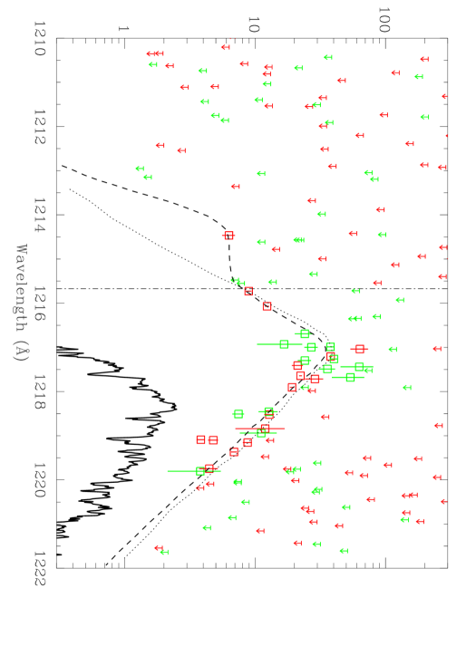
Figure 4: Reconstruction of the H I Ly$\alpha$ profile seen by the fluoresced H₂ surrounding Mira B. The boxes are the inferred Ly$\alpha$ fluxes overlying Lyman band (red) and Werner band (green) H₂ pumping transitions, which fluoresce observed sequences of H₂ lines. Error bars indicate the 1$\sigma$ uncertainty in the fluxes due to uncertainties in the measurements of the H₂ emission lines. Upper limits are shown for undetected sequences. The dashed line is our best estimate for the Ly$\alpha$ profile, which is compared with the profile derived from Paper II (dotted line). The solid line is the actual Ly$\alpha$ line observed by HST/STIS, and the dot-dashed line indicates the rest frame of the star.

The $F_{obs}$ and $f_{dis}$ values in Table 2 can be used to compute the Ly$\alpha$ flux that must be overlying each H₂ pumping transition within Ly$\alpha$, thereby allowing us to reconstruct the Ly$\alpha$ profile seen by the H₂, $f_{0}(\lambda)$. Once again we refer the reader to Paper II for details of this computation, although here we assume our revised values of $T=3900$ K and $\log N(H_{2})=17.1$ in the calculations. Figure 4 shows the new reconstructed Ly$\alpha$ profile. The analysis assumes that the fluoresced H₂ completely surrounds the star and that the H₂ emission emerges isotropically. If these assumptions are inaccurate, the derived profile will be different from the actual profile by some geometric scaling factor, $\eta$, explaining why the y-axis of Figure 4 is labeled $\eta f_{0}$. The red and green boxes in Figure 4 show the inferred flux overlying Lyman and Werner band transitions, respectively, which pump observed fluorescence sequences. These data points collectively map out a self-consistent Ly$\alpha$ line profile, albeit with some scatter. The consistency of the Werner band data points, which are entirely from the FUSE data, and the Lyman band data points, which are mostly from the STIS data, provides further evidence that the Ly$\alpha$ profile is the same at the time of the FUSE and STIS observations.

Our best estimate for the reconstructed Ly$\alpha$ profile is indicated by the dashed line in Figure 4. This is not very different from the profile derived in Paper II (also shown in Fig. 4). The biggest difference between the two profiles is below 1215.5 Å, which is entirely due to the addition of the new 3–1 R(15) Lyman band sequence fluoresced at 1214.4648 Å. This is the only sequence fluoresced at wavelengths blueward of the stellar rest frame. Its existence demonstrates that the H₂ sees at least some Ly$\alpha$ flux on the blue side of the line. As described in Paper II, the reason the observed and reconstructed Ly$\alpha$ lines are highly redshifted is because of absorption from Mira B’s wind on the blue side of the line. The upper limits in Figure 4 are from Lyman and Werner band transitions within Ly$\alpha$ that do not fluoresce enough H₂ emission to be detectable. These upper limits are consistent with the Ly$\alpha$ profile derived from the detected fluorescence sequences.

Photodissociation rates were overestimated in Paper II due to the use of inaccurate dissociation fractions (see above). Thus, it is worthwhile to derive better estimates for H₂ photodissociation rates using the revised analysis presented here. We computed these rates for the detected sequences listed in Table 2, using the $F_{obs}$ and $f_{dis}$ values in that table, and we found that some of the weaker sequences that are newly detected in our FUSE data [e.g., 5–0 P(20)] are surprisingly strong contributors to the total H₂ dissociation rate. This suggests that undetected sequences might collectively contribute substantially to H₂ dissociation via Ly$\alpha$ fluorescence. Therefore, the best way to accurately estimate the H₂ photodissociation rate is to perform a forward modeling exercise computing contributions for all H₂ transitions within Ly$\alpha$, not just the ones that yield detected H₂ emission. The numerous upper limits in Figure 4 provide some idea for how many H₂ transitions must be considered.

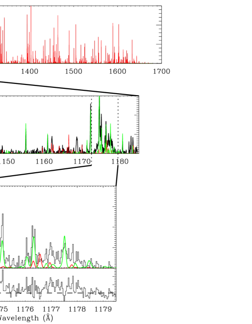
Figure 5: A simulated H₂ spectrum fluoresced by the Ly$\alpha$ line of Mira B (top panel), where the red and green lines are for Lyman and Werner band lines, respectively. In the lower two panels, this simulated spectrum is compared with the FUSE spectrum of Mira B. The bottom panel zooms in on the 1176 Å emission feature, and the residuals of the data after subtraction of the model spectrum are shown. The generally positive flux remaining after subtraction suggests that H₂ is not responsible for all the flux of the 1176 Å feature, and that broad C III $\lambda$1175 emission is contributing to the line.

We perform this calculation using the Monte Carlo radiative transfer routine described above and in Paper II, assuming the Ly$\alpha$ profile derived in Figure 4, and assuming the $T=3900$ K and $\log N(H_{2})=17.1$ values from the line ratio analysis to compute the H₂ level populations. Figure 5 shows a simulated UV H₂ spectrum computed from this calculation. We estimate that the total Ly$\alpha$ flux absorbed and reemitted by H₂ is $1.06\times 10^{-12}$ ergs cm^-2 s^-1, about 31% higher than the flux one would estimate from the detected sequences alone. About 6.8% of the fluorescences lead to H₂ dissociation rather than the emergence of an H₂ line photon, suggesting a dissociation rate of $8.6\times 10^{39}$ s^-1 (at Mira’s distance of 128 pc), or $4.5\times 10^{-10}$ M_⊙ yr^-1. Surprisingly, this is a factor of 2.1 times higher than the value one would derive from the detected sequences alone. Although the undetected sequences absorb less Ly$\alpha$ flux, they tend to have higher dissociation fractions and therefore contribute significantly to the dissociation rate. Nevertheless, the largest contributor to H₂ dissociation is the detected 4–0 P(19) Lyman band sequence, which accounts for 23.5% of the total dissociation rate.

Although the dissociation fractions assumed in Paper II were too high, this is mitigated by the legitimate increase in dissociation rate provided by consideration of undetected fluorescence sequences. Thus, the dissociation rate quoted above is only a factor of 2 lower than reported in Paper II. In Paper II, we proposed that the H₂ emission is arising within a photodissociation front within Mira A’s wind as it approaches Mira B, and we constructed a model of this front consistent with the observations. We experiment with new photodissociation front models assuming our revised estimates for photodissociation rates, and we find that the factor of 2 change is not enough to significantly alter the model. Thus, the photodissociation front model remains a very viable interpretation for the H₂ emission. As mentioned in §1, the implied H₂ dissociation rate is comparable to Mira B’s total accretion rate, consistent with the idea that the UV H₂ emission is showing us H₂ in Mira A’s wind being fluoresced, heated, and dissociated by Ly$\alpha$ as it approaches and is ultimately accreted by Mira B.

We now discuss some of the limitations of our H₂ modeling efforts, because our estimation of $T$ and $N(H_{2})$ and our reconstruction of the Ly$\alpha$ profile in Figure 4 rely on several assumptions. For example, our plane-parallel modeling essentially assumes that Mira B is surrounded by an isothermal H₂ layer of uniform $N(H_{2})$ and that H₂ level populations are precisely thermal. In reality, the H₂ may have a distribution of temperatures (as the photodissociation front models actually predict), it may be distributed inhomogenously around the star, and the fluorescence process itself could lead to some level of nonthermality in the level populations. The limitations introduced by our simplifying assumptions are presumably responsible for the significant scatter of Ly$\alpha$ flux data points in Figure 4 about the best-fit dashed line Ly$\alpha$ profile, beyond the measurement uncertainties. Since the reconstructed profile imprecisely reproduces the data points in Figure 4, the H₂ fluxes of the synthetic spectrum described above are naturally imprecise as well. For example, the synthetic spectrum predicts lines at 1130 Å and 1135 Å that are significantly stronger than observed and a line at 1162 Å significantly weaker than observed (see Fig. 5). Another source of uncertainty is line blending, which is not considered in our radiative transfer calculations. For example, there are 2 Lyman band data points at 1219 Å in Figure 4 that are too low, probably because these H₂ pumping transitions are blended enough that they are partially shielding each other from the full Ly$\alpha$ flux present at that wavelength. Emission line blends could also lead to H₂ photons shifting from one fluorescence sequence to another. All the effects and assumptions described above could lead to inaccuracies in our derived H₂ properties.

5 THE C III LINES AND MIRA B’S VARIABILITY

One goal of our FUSE observations was to try to detect broad, high temperature emission lines formed in the accretion disk of Mira B. We see no evidence of the O VI $\lambda\lambda$1032,1038 lines, which are typically very strong lines in coronal spectra. We estimate a 3$\sigma$ upper limit of $9\times 10^{-16}$ ergs cm^-2 s^-1 for these lines. The only possible accretion lines are the two C III lines shown in Figure 1. The widths of these two lines are roughly consistent with observations of high temperature lines from IUE (Reimers & Cassatella, 1985), but the identification with C III is still somewhat tentative. We identify the broad bump at 976.447 Å as C III $\lambda$977, but if it is C III it has a very large blueshift of $-232$ km s^-1, assuming a stellar velocity of $+56$ km s^-1 (Bowers & Knapp, 1988; Planesas et al., 1990; Josselin et al., 2000). The scattered solar C III $\lambda$977 line is sometimes seen in FUSE spectra, but the observed feature is far too broad for that to be responsible. The spike seen on the red edge of the line could perhaps be the solar emission.

One possible explanation for the blueshift of the C III line is that we are seeing emission predominantly from the side of the accretion disk that is rotating towards us. There is no corresponding blueshift of the C III $\lambda$1175 line (see below), but the $\lambda$977 line is a high opacity resonance line, meaning intervening C III material could in principle scatter background $\lambda$977 emission, while the $\lambda$1175 lines are lower opacity intersystem lines, so the same process may not work for $\lambda$1175. Another possible explanation for the C III blueshift is absorption from overlying H₂. The density of H₂ transitions increases towards the shorter wavelengths accessible to FUSE. These transitions will have higher opacities than any of the observed H₂ lines, since they will be originating from lower, more populated levels of the ground electronic state. Below about 1110 Å there are Lyman and Werner band transitions from the lowest levels that will be populated even at very cool temperatures. The column densities of H₂ in these lowest levels could be much higher than for the $T=3900$ K population that we have detected via Ly$\alpha$ fluorescence. This is because most of the H₂ within Mira A’s wind, in which Mira B is embedded, will be at low $T\sim 100$ K temperatures, and only the lowest energy levels will be populated in this cold H₂. Because of the significant H₂ opacity in the neighborhood of the C III $\lambda$977 line, the red side of the line might be absorbed, making the resulting C III profile appear as blueshifted as seen in our FUSE data. Despite these plausible explanations for the blueshift, the detection of the $\lambda$977 line will remain tentative until a more definitive explanation of the blueshift is available.

The C III $\lambda$1175 multiplet is blended with many H₂ emission lines and it is therefore unclear that C III is actually contributing to the observed emission. At the end of §4 we described a forward modeling calculation designed to compute the total H₂ photodissociation rate from Ly$\alpha$ fluorescence, including contributions from undetected fluorescence sequences. This calculation also provides us with the synthetic H₂ emission spectrum shown in Figure 5. This figure compares the synthetic spectrum with the FUSE data, demonstrating a reasonably good fit to the observed H₂ lines. The bottom panel focuses on the 1176 Å region. We subtract the H₂ spectrum from the data to see if the H₂ lines can account for all of the line flux. The residual flux shown below the lowest panel of Figure 5 suggests that there is flux remaining after this subtraction that we can associate with the C III $\lambda$1175 multiplet. The integrated flux remaining is $1.4\times 10^{-14}$ ergs cm^-2 s^-1, in good agreement with the C III flux suggested by the two-Gaussian representation in Figure 2, providing support for this being a reasonably accurate C III flux measurement. The flux ratio of C III $\lambda$977 and C III $\lambda$1175 is often used as a density diagnostic, but in Mira B’s case the significant uncertainties involved in measuring both lines are too large to obtain a believable density measurement.

The 1176 Å emission feature is the only feature in our FUSE spectrum that is also detectable in the previous HST/STIS spectrum (see Fig. 2 in Paper I). The sensitivity of STIS drops dramatically below 1200 Å, so the S/N of the STIS spectrum at 1176 Å is very low. The data quality does not allow us to separate the H₂ emission from the C III emission, so we can only report a total STIS flux of $(2.7\pm 0.8)\times 10^{-14}$ ergs cm^-2 s^-1 for the 1176 Å line. This agrees well with the integrated FUSE flux of $(3.00\pm 0.13)\times 10^{-14}$ ergs cm^-2 s^-1. In §3 and §4, we demonstrated that the H I Ly$\alpha$ line had not changed between the times of the STIS and FUSE observations. The excellent flux agreement for the 1176 Å feature provides further evidence that the UV spectrum of Mira B is unchanged.

The C III $\lambda$1175 line has also been observed numerous times by IUE. We found 32 short-wavelength, low-resolution (SW-LO) observations of Mira B in the IUE archive. Only about half of them are long enough exposures with sufficient S/N to measure a C III flux. Note that while H₂ may be contaminating the C III line in the HST/STIS and FUSE data, we do not believe that this is the case for the IUE data. In Paper I it was argued that unblended H₂ features should have been seen in the IUE data if H₂ were contributing flux to other emission features such as C III $\lambda$1175.

In Figure 6, we plot the C III fluxes as a function of time, where for purposes of this figure we have made no attempt to correct the STIS and FUSE fluxes for H₂ contamination. The STIS and FUSE fluxes are about an order of magnitude lower than the IUE fluxes, consistent with the drop in flux seen in the continuum and many other emission lines (see Paper I). The drop in flux is presumably due to a substantial decrease in accretion rate, which also led to a similar decrease in mass loss rate for Mira B (see Paper II). The consistency of the 1999 STIS and 2001 FUSE data demonstrates that this decrease is an enduring phenomenon.

It is possible that similar changes in accretion rate have been detected from optical data. Mira B is difficult to observe from the ground due to its close proximity with the generally brighter Mira A, but during Mira A minimum it is possible to detect the presence of Mira B. Joy (1954) and Yamashita & Maehara (1977) report a possible periodic variation in Mira B’s optical light curve with a period of 14 years and with an intensity range of about a factor of 4. Considering that these optical intensities will be contaminated with Mira A emission even at Mira A minimum, these variations might be consistent with the factor of 20 variations seen in the UV.

However, if the period of these variations is 14 years, why did the long-lived IUE not see them? Yamashita & Maehara (1977) report a Mira B optical minimum in 1971, so in Figure 6 we display a 14-year period sine curve consistent with this phasing. All the IUE data points occur near predicted maxima, while the STIS and FUSE data points are near a predicted minimum. There is an unfortunate time gap in the IUE data from 1981–1990 that means the predicted Mira B minimum period was not covered by the IUE SW-LO data set. Thus, it is possible that the substantial drop in flux seen by STIS and FUSE is simply the UV manifestation of the 14-year optical cycle detected by Joy (1954) and Yamashita & Maehara (1977). One argument against this is that while there are no SW-LO IUE observations from 1981–1990, there are long-wavelength, low-resolution (LW-LO) spectra from 1983 July 9 and 1988 January 8. Although Mg II $\lambda$2800 and continuum fluxes are somewhat lower than average in these spectra, neither spectrum shows flux levels dramatically below those of other LW-LO observations in the IUE data set. This leaves only about a 5-year time gap in the IUE coverage during which Mira B fluxes could have dropped tremendously like they did in 1999–2001. Nevertheless, it would be worthwhile to observe Mira B again with FUSE and/or HST in 2004–2007 to see if high UV fluxes return as Figure 6 predicts.

6 SUMMARY

We have analyzed UV observations of the wind-accreting star Mira B, using new FUSE spectra combined with previous HST/STIS data. Our results are summarized as follows:

1.

In the new FUSE data, we detect Ly$\alpha$-fluoresced H₂ lines that are mostly Werner band lines rather than the Lyman band lines previously detected by HST. Most of the FUSE H₂ lines have never before been identified in an astrophysical spectrum.

2.

Using previously developed techniques, we analyze the Mira B H₂ emission, combining the old HST/STIS and the new FUSE H₂ data. We estimate a temperature and column density for the H₂ layer responsible for the emission of $T=3900$ K and $\log N(H_{2})=17.1$, respectively.

3.

Our modeling efforts demonstrate that undetected H₂ fluorescence sequences actually produce more H₂ photodissociation from Ly$\alpha$ fluorescence than do the detected sequences. Considering both, we estimate a total photodissociation rate of $4.5\times 10^{-10}$ M_⊙ yr^-1, comparable to the $(8-30)\times 10^{-10}$ M_⊙ yr^-1 total accretion rate of Mira B. The FUSE and HST H₂ emission may be coming from a photodissociation front, as first proposed in the analysis of the HST data (see Paper II).

4.

The only stellar lines detected in our FUSE spectrum other than H₂ are the broad C III $\lambda$977 and C III $\lambda$1175 lines, which originate from within Mira B’s accretion disk. The C III $\lambda$977 line is highly blueshifted from its expected location, which leads us to consider its identification as tentative. Overlying H₂ absorption or particularly bright emission from one side of the accretion disk could in principle be responsible for the blueshift. The C III $\lambda$1175 line is heavily blended with numerous H₂ emission lines, making an accurate flux measurement difficult.

5.

Analysis of the H₂ and C III $\lambda$1175 lines in the 1999 HST/STIS and 2001 FUSE data demonstrates that the UV spectrum of Mira B is roughly the same at these two times. The UV fluxes of both data sets are dramatically lower than ever observed by IUE in 1979–1995. The presence of the lower fluxes over at least two years (1999–2001) demonstrates that they are a persistent phenomenon.

6.

We hypothesize that the drop in UV flux in 1999–2001 is associated with a previously identified 14-year periodic variation in optical emission from Mira B, and that IUE missed the variation due to most IUE observations falling near the two maxima of the cycle during the IUE era.

Table 1: Line List

$\lambda_{meas}$	$f_{obs}$	FWHM	ID	$\lambda_{rest}$	$f_{mod}$	Fluoresced by
(Å)	($10^{-15}$)	(km s-1)		(Å)	($10^{-15}$)
FUSE H2 Lines
$1127.433\pm 0.008$	$2.87\pm 0.23$	$50\pm 5$	0-2 Q(10)	1127.160	1.60	0-4 Q(10) $\lambda$1217.263
			1-3 P(5)	1127.245	0.78	1-5 P(5) $\lambda$1216.988
$1130.571\pm 0.015$	$0.66\pm 0.14$	$31\pm 7$	1-3 Q(7)	1130.365	1.65	1-5 Q(7) $\lambda$1218.507
$1131.608\pm 0.015$	$0.98\pm 0.18$	$37\pm 8$	2-4 R(1)	1131.309	0.22	2-6 R(1) $\lambda$1217.298
			1-3 R(9)	1131.390	1.03	1-5 R(9) $\lambda$1216.997
$1143.257\pm 0.021$	$0.61\pm 0.16$	$39\pm 9$	2-4 P(5)	1142.956	0.38	2-6 R(3) $\lambda$1217.488
			2-0 P(11)	1143.112	0.07	2-2 R(9) $\lambda$1219.101
$1155.154\pm 0.008$	$1.53\pm 0.23$	$24\pm 4$	1-3 P(11)	1154.910	1.84	1-5 R(9) $\lambda$1216.997
$1160.912\pm 0.010$	$1.01\pm 0.20$	$24\pm 5$	1-4 R(3)	1160.647	1.38	1-5 P(5) $\lambda$1216.988
$1162.051\pm 0.019$	$2.18\pm 0.32$	$61\pm 10$	0-1 R(0)	1161.693	0.72	0-2 R(0) $\lambda$1217.205
			1-1 P(5)	1161.814	0.16	1-2 P(5) $\lambda$1216.070
			1-1 R(6)	1161.949	0.21	1-2 R(6) $\lambda$1215.726
$1172.242\pm 0.006$	$4.60\pm 0.40$	$41\pm 4$	1-4 P(5)	1171.953	1.62	1-5 P(5) $\lambda$1216.988
			0-3 Q(10)	1172.031	2.67	0-4 Q(10) $\lambda$1217.263
$1174.571\pm 0.007$	$4.29\pm 0.50$	$37\pm 5$	2-5 R(1)	1174.298	1.41	2-6 R(1) $\lambda$1217.298
			1-4 Q(7)	1174.347	4.04	1-5 Q(7) $\lambda$1218.507
$1174.846\pm 0.013$	$1.25\pm 0.35$	$28\pm 9$	2-5 R(0)	1174.574	0.29	2-6 R(0) $\lambda$1217.680
			2-5 R(2)	1174.588	0.30	2-6 R(2) $\lambda$1217.440
$1175.110\pm 0.007$	$2.07\pm 0.35$	$25\pm 4$	2-5 R(3)	1174.869	1.64	2-6 R(3) $\lambda$1217.488
$1176.060\pm 0.013$	$0.89\pm 0.28$	$25\pm 8$	2-5 Q(1)	1175.826	0.78	2-6 Q(1) $\lambda$1218.940
$1176.319\pm 0.010$	$2.22\pm 0.36$	$34\pm 6$	5-0 R(18)	1176.066	0.57	5-0 P(20) $\lambda$1217.717
			0-2 Q(18)	1176.082	1.58	0-3 Q(18) $\lambda$1216.692
			2-5 R(4)	1176.085	0.33	2-6 R(4) $\lambda$1218.457
$1176.978\pm 0.016$	$0.60\pm 0.25$	$20\pm 10$	6-0 R(19)	1176.706	0.53	6-0 P(21) $\lambda$1218.841
			2-5 Q(2)	1176.788	0.19	2-6 Q(2) $\lambda$1219.804
$1177.518\pm 0.026$	$0.95\pm 0.36$	$39\pm 17$	1-3 Q(16)	1177.269	1.75	1-4 Q(16) $\lambda$1216.930
$1180.710\pm 0.013$	$0.64\pm 0.18$	$16\pm 7$	2-5 P(3)	1180.457	1.38	2-6 R(1) $\lambda$1217.298
Other FUSE Lines
$976.447\pm 0.121$	$6.99\pm 1.60$	$338\pm 84$	C III?	977.020
$1174.616\pm 0.083$	$7.03\pm 1.82$	$287\pm 47$	C III?	1175mult
$1177.206\pm 0.115$	$8.57\pm 1.32$	$405\pm 68$	C III?	1175mult
New STIS H2 Lines
$1254.369\pm 0.013$	$1.01\pm 0.31$	$16\pm 4$	3-1 P(17)	1254.125	0.26	3-1 R(15) $\lambda$1214.465
$1265.421\pm 0.009$	$0.99\pm 0.27$	$17\pm 5$	3-2 R(15)	1265.180	0.31	3-1 R(15) $\lambda$1214.465
$1593.575\pm 0.016$	$3.77\pm 0.83$	$23\pm 6$	3-9 R(15)	1593.258	0.74	3-1 R(15) $\lambda$1214.465
$1621.385\pm 0.021$	$3.54\pm 0.89$	$26\pm 8$	3-10 R(15)	1621.119	0.39	3-1 R(15) $\lambda$1214.465
$1622.434\pm 0.011$	$5.19\pm 1.01$	$26\pm 6$	3-9 P(17)	1622.133	0.87	3-1 R(15) $\lambda$1214.465

Table 2: Fluorescence Sequences

Fluorescing	$\lambda_{rest}$	$F_{obs}$	Absorption	$E_{low}$	$g_{low}$	$f_{dis}^{\prime}$	$f_{dis}$
Transition	(Å)	($10^{-13}$)	Strength (f)	(cm-1)
Lyman Band Sequences from Paper II
1-2 R(6)	1215.7263	0.502	0.0349	10261.20	13	0.0	0.0
1-2 P(5)	1216.0696	0.914	0.0289	9654.15	33	0.0	0.0
3-3 P(1)	1217.0377	0.115	0.0013	11883.51	9	0.0	0.0
0-2 R(0)	1217.2045	0.858	0.0441	8086.93	1	0.0	0.0
4-0 P(19)	1217.4100	0.190	0.0093	17750.25	117	0.417	0.469
0-2 R(1)	1217.6426	1.355	0.0289	8193.81	9	0.0	0.0
2-1 P(13)	1217.9041	1.141	0.0192	13191.06	81	0.002	0.002
2-1 R(14)	1218.5205	0.324	0.0181	14399.08	29	0.006	0.006
0-2 R(2)	1219.0887	0.165	0.0256	8406.29	5	0.0	0.0
2-2 R(9)	1219.1005	0.320	0.0318	12584.80	57	0.0	0.0
2-2 P(8)	1219.1543	0.340	0.0214	11732.12	17	0.0	0.0
0-2 P(1)	1219.3676	0.318	0.0149	8193.81	9	0.0	0.0
0-1 R(11)	1219.7454	0.166	0.0037	10927.12	69	0.0	0.0
New Lyman Band Sequences
3-1 R(15)	1214.4648	0.284	0.0236	15649.58	93	0.031	0.037
5-0 P(20)	1217.7165	0.069	0.0115	19213.16	41	0.478	0.499
6-0 P(21)	1218.8403	0.051	0.0130	20688.04	129	0.520	0.555
Werner Band Sequences
0-3 Q(18)	1216.6926	0.036	0.0396	25499.74	37	0.0	0.0
1-4 Q(16)	1216.9302	0.034	0.0712	25929.42	33	0.0	0.0
1-5 P(5)	1216.9878	0.072	0.0071	19807.03	33	0.016	0.031
1-5 R(9)	1216.9969	0.099	0.0197	22251.21	57	0.017	0.031
0-4 Q(10)	1217.2628	0.065	0.0100	20074.45	21	0.0	0.0
2-6 R(1)	1217.2978	0.052	0.0558	21589.82	9	0.008	0.012
2-6 R(2)	1217.4400	0.047	0.0399	21756.98	5	0.066	0.089
2-6 R(3)	1217.4883	0.090	0.0364	22005.58	21	0.073	0.113
2-6 R(0)	1217.6800	0.027	0.1098	21505.78	1	0.002	0.002
2-6 R(4)	1218.4566	0.015	0.0399	22332.85	9	0.017	0.025
1-5 Q(7)	1218.5084	0.055	0.0303	20894.94	45	0.0	0.0
2-6 Q(1)	1218.9402	0.023	0.0532	21589.82	9	0.0	0.0
2-6 Q(2)	1219.8038	0.004	0.0532	21756.98	5	0.0	0.0

Figure 1: Two regions of the FUSE spectrum of Mira B. Line identifications are displayed, where the $\oplus$ symbol indicates a line is an airglow line rather than a stellar feature.

Figure 2: Multi-Gaussian fit to the 1176 Å emission feature. The 7 narrow components are H₂ lines, and we assume the sum of the 2 broad components is representative of the C III $\lambda$1175 line profile.

Figure 3: Reduced $\chi^{2}$ contours measuring how well the H₂ lines ratios can be reproduced as a function of assumed temperature and column density. Both FUSE and HST/STIS H₂ lines are considered in the analysis. The best fit is at $T=3900$ K and $\log N(H_{2})=17.1$ (plus sign).

Figure 6: C III $\lambda$1175 flux plotted as a function of time, where triangles are IUE measurements, the box is from the HST/STIS spectrum, and the diamond is from the FUSE data. Note that for the HST and FUSE data, the C III feature is heavily contaminated with H₂ lines, while this is probably not the case for the IUE data. The sine curve is a schematic representation of the 14 year periodicity for Mira B suggested by optical observations (Joy 1954; Yamashita & Maehara 1977).

References

- Abgrall, Roueff, & Drira (2000) Abgrall, H. A., Roueff, E., & Drira, I. 2000, A&AS, 141, 297
- Abgrall et al. (1993a) Abgrall, H. A., Roueff, E., Launay, F., Roncin, J. -Y., & Subtil, J. -L. 1993a, A&AS, 101, 273
- Abgrall et al. (1993b) Abgrall, H. A., Roueff, E., Launay, F., Roncin, J. -Y., & Subtil, J. -L. 1993b, A&AS, 101, 323
- Ardila et al. (2002a) Ardila, D. R., Basri, G., Walter, F. M., Valenti, J. A., & Johns-Krull, C. M. 2002, ApJ, 566, 1100
- Bartoe et al. (1979) Bartoe, J. -D., F. Brueckner, G. E., Nicolas, K. R., Sandlin, G. D., VanHoosier, M. E., & Jordan, C. 1979, MNRAS, 187, 463
- Bevington & Robinson (1992) Bevington, P. R., & Robinson, D. K. 1992, Data Reduction and Error Analysis for the Physical Sciences (New York: McGraw-Hill)
- Bowers & Knapp (1988) Bowers, P. F., & Knapp, G. R. 1988, ApJ, 332, 299
- Brown et al. (1981) Brown, A., Jordan, C., Millar, T. J., Gondhalekar, P., & Wilson, R. 1981, Nature, 290, 34
- Dabrowski (1984) Dabrowski, I. 1984, Can. J. Phys., 62, 1639
- Herczeg et al. (2002) Herczeg, G. J., Linsky, J. L., Valenti, J. A., Johns-Krull, C. M., & Wood, B. E. 2002, ApJ, 572, 310
- Herczeg et al. (2003) Herczeg, G. J., Wood, B. E., Linsky, J. L., Valenti, J. A., & Johns-Krull, C. M. 2003, ApJ, submitted
- Jordan et al. (1977) Jordan, C., Brueckner, G. E., Bartoe, J.-D. F., Sandlin, G. D., & VanHoosier, M. E. 1977, Nature, 270, 326
- Josselin et al. (2000) Josselin, E., Mauron, N., Planesas, P., & Bachiller, R. 2000, A&A, 362, 255
- Joy (1954) Joy, A. H. 1954, ApJS, 1, 39
- Jura & Helfand (1984) Jura, M., & Helfand, D. J. 1984, ApJ, 287, 785
- Karovska et al. (1997) Karovska, M., Hack, W., Raymond, J., & Guinan, E. 1997, ApJ, 482, L175
- Knapp (1985) Knapp, G. R. 1985, ApJ, 293, 273
- Knapp et al. (1998) Knapp, G. R., Young, K., Lee, E., & Jorissen, A. 1998, ApJS, 117, 209
- McMurry, Jordan, & Carpenter (1999) McMurry, A. D., Jordan, C., & Carpenter, K. G. 1999, MNRAS, 302, 48
- Moos et al. (2000) Moos, H. W., et al. 2000, ApJ, 538, L1
- Morrissey et al. (1997) Morrissey, P. F., Feldman, P. D., Clarke, J. T., Wolven, B. C., Strobel, D. F., Durrance, S. T., & Trauger, J. T. 1997, ApJ, 476, 918
- Perryman et al. (1997) Perryman, M. A. C., et al. 1997, A&A, 323, L49
- Planesas et al. (1990) Planesas, P., Bachiller, R., Martin-Pintado, J., & Bujarrabal, V. 1990, ApJ, 351, 263
- Reimers & Cassatella (1985) Reimers, D., & Cassatella, A. 1985, ApJ, 297, 275
- Ryde & Schöier (2001) Ryde, N., & Schöier, F. L. 2001, ApJ, 547, 384
- Valenti, Johns-Krull, & Linsky (2000) Valenti, J. A., Johns-Krull, C. M., & Linsky, J. L. 2000, ApJS, 129, 399
- Warner (1972) Warner, B. 1972, MNRAS, 159, 95
- Wilkinson et al. (2002) Wilkinson, E., Harper, G. M., Brown, A., & Herczeg, G. J. 2002, AJ, 124, 1077
- Wood & Karovska (2000) Wood, B. E., & Karovska, M. 2000, ApJ, 535, 304
- Wood, Karovska, & Hack (2001) Wood, B. E., Karovska, M., & Hack, W. 2001, ApJ, 556, L51 (Paper I)