Helioseismic Probing of Solar Variability: The Formalism and Simple Assessments

Abstract

We derive formulae connecting the frequency variations in the spectrum of solar oscillations to the dynamical quantities that are expected to change over the solar activity cycle. This is done for both centroids and the asymmetric part of the fine structure (so-called even-$a$ coefficients). We consider the near-surface, small-scale magnetic and turbulent velocity fields, as well as horizontal magnetic fields buried near the base of the convective zone. For the centroids we also discuss the effect of temperature variation.

We demonstrate that there is a full, one-to-one correspondence between the expansion coefficients of the fine structure and those of both the averaged small-scale velocity and magnetic fields. Measured changes in the centroid frequencies and the even-$a$’s over the rising phase solar cycle may be accounted for by a decrease in the turbulent velocity of order 1%. We show that the mean temperature decrease associated with the net decrease in the efficiency of convective transport may also significantly contribute to the increase of the centroid frequencies. Alternatively, the increase may be accounted for by an increase of the small-scale magnetic field of order 100 G, if the growing field is predominantly radial.

We also show that global seismology can be used to detect a field at the level of a few times $10^{5}$ G, if such a field were present and confined to a thin layer near the base of the convective envelope.

1 Introduction

We study global changes, over the solar cycle, in the sun’s eigenmode frequencies – centroids and asymmetric fine structure – in a search of physical changes occurring beneath the photosphere. There is abundant phenomenological information about the helioseismic changes, but there is no satisfactory physical model describing the changes. We consider three possible dynamical sources of the evolution – changes in the sub-photospheric small-scale magnetic and velocity fields and a large-scale toroidal field buried in a thin layer near the base of the convection zone. Here, we develop the formalism needed to connect these dynamical changes to frequencies changes.

In our treatment of the small-scale magnetic field, we generalize the method of Goldreich et al.(1991, GMWK) to include the generalized effect of the small-scale magnetic field on nonradial modes, while further generalizing to a non-spherical distribution of the averaged field. Although it is true that radial modes may adequately represent lower degree (up to about $\ell=60)$ nonradial p-modes, if the magnetic field effects were confined to the outermost layers, this is not true for higher degree p-modes or most f-modes. Still, the more important generalization is that we treat a non-isotropic, non-spherical field distribution, which allows us to interpret the observed evolution of the anti-symmetric part of the fine structure in the spectrum of solar oscillations (so-called even-$a$ coefficients).

Furthermore, we study effects a small-scale, random velocity field. A role for the changing turbulent velocities has been suggested by Kuhn (1999). However, a first-principles treatment still needs to be made. We give an estimate of the associated temperature change and its effect on oscillation frequencies.

Finally, we consider the effect of a buried toroidal field, which may be expected to be confined near the base of the convective envelope. The present work represents an advance over earlier ones (Gough & Thompson ,1990; Dziembowski & Goode, 1991) because we make a more explicit and useful formulation by eliminating derivatives of the unknown dynamical quantities. This improved development allows us to obtain more physically revealing formulae. The application of this part of our work is determining a stringent limit on the size of a buried toroidal field.

2 The Helioseismic Data

Solar frequency data are usually given in the form

$$\nu_{\ell n}^{m}=\bar{\nu}_{\ell n}+\sum_{k=1}a_{k,\ell n}{\cal P}_{k}^{\ell}(m),$$ (1)

where the ${\cal P}$ are orthogonal polynomials (see Ritzwoller & Lavely 1991 and Schou et al. 1994). The remaining symbols ($n\ell m$), in this equation have their usual meanings. This representation ensures that $\bar{\nu}_{\ell,n}$ – the centroid frequencies – are a probe of the spherical structure, while the $a_{2k}$ – the even-$a$ coefficients – are a probe of the symmetrical (about the equator) part of distortion described by the corresponding $P_{2k}(\cos\theta)$ Legendre polynomials. We note that in lowest order, perturbations that are symmetrical about the equator induce an asymmetric change in the fine structure of the oscillation spectrum.

For the angular integrals, we have

$$Q^{m}_{k,\ell}\equiv\int_{0}^{2\pi}\int_{-1}^{1}|Y_{\ell}^{m}|^{2}P_{2k}d\mu d\phi=S_{k,\ell}{\cal P}_{2k}^{\ell}(m)$$ (2)

where $\mu=\cos\theta$ and

$$S_{k,\ell}=(-1)^{k}{(2k-1)!!\over k!}{(2\ell+1)!!\over(2\ell+2k+1)!!}{(\ell-1)!\over(\ell-k)!}.$$

Following our earlier works (see e.g. Goode & Dziembowski, 2002), we use here the following convenient quantities, $\gamma_{k,\ell n}$, through the following two relations,

$$\Delta\bar{\nu}_{\ell n}={\gamma_{0,\ell n}\over\tilde{I}_{\ell n}}$$ (3)

and

$$a_{2k,\ell n}=S_{k,\ell}{\gamma_{k,\ell n}\over\tilde{I}_{\ell n}},$$ (4)

where $\tilde{I}_{\ell,n}$ is the dimensionless mode inertia calculated for our reference model. A clear advantage of the $\gamma$’s is that their growth replicates the growth of other measures of solar activity. For the p-modes, the $1/\tilde{I}$ factor takes care of the $\ell$- and most of the $\nu$-dependence in $\Delta\bar{\nu}$ and in the even-$a$ coefficients. The fact that the residual $\nu$-dependence is weak points to a localization of the source of the observed frequency changes close to to the photosphere.

The numerical values of the $\gamma$’s scale with the square of the eigenfunction normalization at the photosphere. The normalization we adopted in our analyses of the SOHO MDI data (e.g. Goode & Dziembowski, 2002) and which is used throughout present paper, is explained in the next section. With this normalization, the value of $\gamma_{0}$ reaches up to the $0.3\mu$Hz range. The absolute values of $\gamma_{1}$ and $\gamma_{3}$ are about twice larger. Having determined the set of $\gamma_{k}$, one may construct seismic maps of the varying sun’s activity (Dziembowski & Goode, 2002), that is the $\gamma(\mu)$ dependence. In such maps, a rising $\gamma$ reflects the local rise of in the activity. The highest values of $\gamma(\mu)$ are about $1\mu$Hz and they are reached at $\mu\approx 0.3$ and at the peak of the activity. At activity minimum the highest $\gamma(\mu)\approx 0.2\mu$Hz occurs in the polar region.

In the subsequent sections, we will connect the $\gamma$’s, to magnetic and velocity fields that are expected to change in the sun over its activity cycle. To achieve this, we start from a variational principle for oscillation frequencies. In our expressions, the $\ell,n$ subscripts and the $m$ superscript will not be given unless it is necessary for clarity.

3 Variational principle for oscillation frequencies

There are two ways of deriving the variational expression for oscillation frequencies. Both rely on the adiabatic approximation, which is adopted throughout our study. The first of the two approaches begins with the linearized equations of fluid motion about a steady configuration (see e.g Lynden-Bell & Ostriker, 1967, LBO). The other uses Hamilton’s principle (see e.g. GMWK; Dewar, 1970). Here, we use the form given by LBO with some simplification of the variational principle, while adding the all-important contribution of the magnetic field, as calculated explicitly by Dewar (1970). The LBO form is valid for strictly steady velocity fields. However, we make certain simplifications, which will be explained later, to make it applicable to statistically steady fields. With this, we write

$$\omega^{2}I=-\omega C+D$$ (5)

where

$$I=\int d^{3}\mbox{\boldmath{$x$}}\rho|\mbox{\boldmath{$\xi$}}|^{2}$$ (6)

$$C=2{\rm i}\int d^{3}\mbox{\boldmath{$x$}}\rho\mbox{\boldmath{$\xi$}}^{*}\cdot(\mbox{\boldmath{$v$}}\cdot\mbox{\boldmath{$\nabla$}})\mbox{\boldmath{$\xi$}},$$ (7)

and where $v$ represents the velocity field. The eigenvectors, in a spherically-symmetric and time independent model of the sun, are expressed in the following standard form

$$\mbox{\boldmath{$\xi$}}=r[y(r)\mbox{\boldmath{$e$}}_{r}+z(r)\mbox{\boldmath{$\nabla$}}_{H}]Y_{\ell}^{m}(\theta,\phi)\exp(-{\rm i}\omega t).$$ (8)

We adopt some approximations regarding the eigenfunctions. In addition to adiabaticity, we assume the Cowling approximation is valid, which is well-justified in our application to solar oscillations. Further, we will make use of the fact that the oscillations are either of high degree or high order, which means that

$$|\mbox{\boldmath{$\xi$}}|\ll{\rm Max}(r|\mbox{\boldmath{$\xi$}}_{;r}|,\ell|\mbox{\boldmath{$\xi$}}|).$$

Equivalent approximations were also made by GMWK but, in addition, they ignored the angular dependence of the displacement.

Like LBO, we separate the various contribution to $D$,

$$D=D_{p}+D_{g}+D_{v}+D_{M}.$$ (9)

The pressure term,

$$D_{p}=\int d^{3}\mbox{\boldmath{$x$}}p[\Xi+(\Gamma-1)|\mbox{\rm div}\mbox{\boldmath{$\xi$}}|^{2}],$$ (10)

is the same as in LBO. The quantity $\Gamma$, usually denoted as $\Gamma_{1}$, is the adiabatic exponent. The quantity $\Xi$ is a completely contracted double dyadic product,

$\mbox{\boldmath{$\nabla$}}\mbox{\boldmath{$\xi$}}^{*}:\mbox{\boldmath{$\nabla$}}\mbox{\boldmath{$\xi$}}$. Adopting the standard summation convention, we have

$$\Xi=\xi_{j;k}^{*}\xi_{k;j}=(\xi_{j}^{*}\xi_{k;j}-\xi_{k}^{*}\mbox{\rm div}\mbox{\boldmath{$\xi$}})_{;k}+|\mbox{\rm div}\mbox{\boldmath{$\xi$}}|^{2},$$

where the subscript “;” denotes covariant derivatives. However, with our approximation regarding $\xi$, contributions from the terms involving the Christoffel symbols are negligible, and the derivatives may be regarded as component derivatives. In terms of the radial eigenfunctions, $y$ and $z$, with the adopted approximations we have

$$\Xi \approx [r(yry_{;r}-y\lambda)_{;r}+\lambda^{2}]|Y_{\ell}^{m}|^{2}+$$

$$r(yz)_{;r}|\mbox{\boldmath{$\nabla$}}_{H}Y_{\ell}^{m}|^{2}+[0.5(yrz_{;r}-z\lambda)|Y_{\ell}^{m}|^{2}_{;\theta}$$

$$+z^{2}\mbox{\boldmath{$\nabla$}}_{H}Y^{m*}_{\ell}\cdot\mbox{\boldmath{$\nabla$}}_{H}Y^{m}_{\ell;\theta}]_{;\theta}+[...]_{;\phi},$$

where

$$\lambda=y{gr\over c^{2}}-z{\omega^{2}r^{2}\over c^{2}}$$

is radial eigenfunction corresponding to div$\xi$, $g$ is the local gravity, and $c$ is the speed of sound. The last term in $\Xi$ is obtained from the preceding one by the replacement $\theta\leftrightarrow\phi$. Further, in the adopted approximation, we have

$$ry_{;r}=\lambda+\Lambda z,$$ (11)

where $\Lambda=\ell(\ell+1)$ and

$$rz_{;r}=y-\lambda\left({N\over\omega}\right)^{2}{c^{2}\over gr}.$$ (12)

The term containing the Brunt-Väisälä frequency, $N$, is of the same order as the first one for p-modes only, and only in the outermost layers. However, the whole contribution from the term involving $rz_{;r}$ is small. Hence, we will ignore the term, so that

$$\Xi = \lambda^{2}|Y_{\ell}^{m}|^{2}+(y^{2}+\lambda z+\Lambda z^{2})$$ (13)

$$(\Lambda|Y_{\ell}^{m}|^{2}+|\mbox{\boldmath{$\nabla$}}_{H}Y_{\ell}^{m}|^{2})+$$

$$[...]_{;\theta}+[...]_{;\phi}.$$

The explicit expressions for the last two terms will not be needed.

The gravity term simplifies to

$$D_{g}=-2\int d^{3}\mbox{\boldmath{$x$}}\rho{g\over r}|\xi_{r}|^{2},$$ (14)

after using the Cowling approximation, while the velocity term,

$$D_{v}=-\int d^{3}\mbox{\boldmath{$x$}}\rho|(\mbox{\boldmath{$v$}}\cdot\mbox{\boldmath{$\nabla$}})\mbox{\boldmath{$\xi$}}|^{2},$$ (15)

is the same as in LBO, where it was derived for a steady field velocity field. We will use the same form in our application to a statistically steady turbulent field. The expression for the magnetic term, which is taken from Dewar (1970), is

$$D_{M} = {1\over 4\pi}\int d^{3}\mbox{\boldmath{$x$}}\bigg{[}|(\mbox{\boldmath{$B$}}\cdot\mbox{\boldmath{$\nabla$}})\mbox{\boldmath{$\xi$}}|^{2}-$$ (16)

$$2\mbox{\rm div}\mbox{\boldmath{$\xi$}}^{*}\mbox{\boldmath{$B$}}\cdot(\mbox{\boldmath{$B$}}\cdot\mbox{\boldmath{$\nabla$}})\mbox{\boldmath{$\xi$}}+$$

$${1\over 2}|\mbox{\boldmath{$B$}}|^{2}(\Xi+|\mbox{\rm div}\mbox{\boldmath{$\xi$}}|^{2})\bigg{]}$$

We now perturb eq. [5] about the static, non-magnetic equilibrium state. The $\Delta$ denotes changes in parameters relative to this state. However, for centroid frequencies, $\Delta$ is defined with respect to activity minimum because we do not have models of the sun predicting centroid frequencies with $\mu$Hz precision. Since we want to consider terms that are quadratic in velocity, in principle, we need to consider a second order perturbational expression, which is

$$\Delta\omega = -{C\over 2I}+{C^{2}\over 8I^{2}\omega}-{\omega\Delta C\over 2I\omega}$$ (17)

$$+{\Delta D_{s}+D_{v}+D_{M}\over 2I\omega}$$

where

$$\Delta D_{s}=\Delta(D_{p}+D_{g})-\omega^{2}\Delta I.$$ (18)

Actually, we do not calculate the $C$ integral or its perturbation, but only comment on the role of the terms in $C$ for various velocity fields. The first term, which is linear in velocity, results from rotation, and gives rise to odd-$a$ coefficients, which we are not treating here. It may be easily shown that both meridional and statistically steady turbulence do not contribute. The second term, $\propto C^{2}$ due to rotation gives a negligible contribution ( Dziembowski and Goode, 1992) to p-mode splitting. The term $\propto\Delta C$ arises from the first order perturbation of the eigenfunctions due to the velocity fields. Here the contribution from rotation and meridional circulation can be shown to be negligible. The only quadratic effect of rotation, which we found to be significant for p-modes is that of the centrifugal distortion. Thus, it is included in the $D_{s}$ term. For the f-mode even-$a$’s, which are not accurately determined, the terms involving $C^{2}$ may be important. The alternative approach, which has been used by us in all our analyses of the even-$a$ coefficients, is to evaluate the centrifugal contribution and subtract it from the data. We neglect contribution from turbulence to the term $\propto\Delta C$, because we include only effects of interaction of oscillations with the averaged velocity fields. It has to be kept in mind, however, that not all effects of turbulence are included in our formalism. So that we are left with the expression

$$\Delta\omega={1\over 2I\omega}\left(\Delta D_{s}+D_{v}+D_{M}\right)$$ (19)

In the $D_{v}$ term, we consider only effects of the turbulent pressure and we will be interested in the part that may vary with the solar activity. We do not have yet observational evidence for changes in turbulent velocity but such changes are expected. The only global changes in velocity which were definitely detected are the torsional oscillations but their effect on frequencies we estimated to be insignificant.

The $D_{s}$ integral may be calculated considering either Eulerian or Lagrangian perturbations. The results must be the same. The $D_{v}$ and $D_{M}$ integrals are treated as perturbations. We may see that the integrands do not involve differentiation of the unknown characteristics of the velocity and magnetic fields, rather the differentiation is placed upon the eigenfunctions, which are known. This is clearly advantageous and we will apply the same strategy in the evaluations of $\Delta D_{s}$.

The calculated frequency perturbation for individual ($\ell nm$)-modes are linked to the $\gamma^{\prime}s$ defined in eqs. [3] and [4] by the following relation

$$\Delta\omega_{\ell n}^{m}={2\pi\over\tilde{I}_{\ell n}}\sum_{k=0}\gamma_{k,\ell n}Q^{m}_{k,\ell},$$ (20)

with

$$I_{\ell n}=R_{\odot}^{5}\bar{\rho}_{\odot}\tilde{I}_{\ell n},$$

$$\tilde{I}_{\ell n}=\int dxx^{4}\tilde{\rho}{\cal E},$$

$$x={r\over R_{\odot}},\qquad\tilde{\rho}={\rho\over\bar{\rho}},$$

and

$${\cal E}=y^{2}+\Lambda z^{2}.$$

As a normalization of the eigenfunctions, we adopt

$$y_{\ell,n}(r_{\rm phot})=2\times 10^{4}.$$

This is an arbitrary choice which leads to maximal $\gamma$’s in the $(0.2-1)\mu$Hz range, which is the same order as the frequency shifts. This normalization is assumed in all expressions for $\gamma$ provided in this paper.

4 Dynamical perturbations of the structure

Here, we include the dynamical effects of the magnetic $B$, and those of the velocity fields, $v$. We write the condition of mechanical equilibrium, in the presence of perturbing force $F$, in the following form,

$$\nabla p+\rho g\mbox{\boldmath{$e$}}_{r}=\mbox{\boldmath{$F$}},$$ (21)

where

$$F \equiv -\left({\partial{\cal V}\over\partial r}\mbox{\boldmath{$e$}}_{r}+{\partial{\cal H}\over\partial\theta}{\mbox{\boldmath{$e$}}_{\theta}\over r}\right)=$$

$$-{1\over 4\pi}\left[{1\over 2}\nabla\mbox{\boldmath{$B$}}^{2}-(\mbox{\boldmath{$B$}}\cdot\nabla)\mbox{\boldmath{$B$}}\right]-\rho(\mbox{\boldmath{$v$}}\cdot\nabla)\mbox{\boldmath{$v$}}$$

We neglected the perturbation of the gravitational potential, which is justified because we considering perturbing forces concentrated in thin layers containing little mass. eq. [21] implies

$$p=-{\cal H}+h(r)$$ (23)

and

$$\rho={1\over g}{\partial\over\partial r}({\cal H}-{\cal V}-h).$$ (24)

The quantities ${\cal V}$ and ${\cal H}$ represent non-gas pressures, which in general are anisotropic. It should be noted that when the non-gas pressure is isotropic, then the mass distribution remains spherically symmetric. The quantity $h(r)$ may only be determined by utilizing the condition of thermal equilibrium. For the non-spherically symmetric parts of the force, the pressure and density follow from the condition of mechanical equilibrium.

From now on, we treat $F$ as a small perturbing force. Primed letters denote Eulerian perturbations of the respective structure parameters, letters preceded by $\delta$ denote Lagrangian perturbations, and letters without such symbols imply unperturbed variables. We use the standard relation

$$\delta f=f^{\prime}+{df\over dr}\delta r$$

and we adopt $\delta M_{r}=0$, for both spherical and aspherical perturbations.

Note that if we make a Legendre expansion in even orders, $P_{2k}(\cos\theta)$, of ${\cal H}$ and ${\cal V}$, all the expansion coefficients ${p^{\prime}_{k}}$ and ${\rho^{\prime}_{k}}$, starting from $k=1$ are completely specified. Here we are considering only even order polynomials because these are the ones that contribute to the even-$a$ coefficients. The anti-symmetric (odd-order) polynomials average out. From eqs. [23] and [24], we get for $k>0$,

$$p^{\prime}_{k}=-{\cal H}_{k}$$

and

$$\rho^{\prime}_{k}={1\over g}{d\over dr}({\cal H}_{k}-{\cal V}_{k}).$$ (25)

The expansion coefficients for the Lagrangian perturbations are calculated as follows. From the radial component of eq. [21] we have

$$\delta_{k}p=-{\cal V}_{k}+4\int_{r}^{R}{\delta_{k}r\over r}g\rho dr\approx-{\cal V}_{k}$$ (26)

and from mass conservation

$${d\delta_{k}r\over dr}=-{\delta_{k}\rho\over\rho}-2{\delta_{k}r\over r}\approx-{\delta_{k}\rho\over\rho}.$$ (27)

The approximate equality in the preceding equation corresponds to neglecting of the perturbation in the mass distribution above the point under consideration. This is certainly valid for all of our applications. The approximate equality in eq. [27] is just the local plane parallel approximation. This is valid for most of applications considered here. The only possible exception will be discussed briefly in subsection 5.1. Both approximations were adopted in GMWK. We stress, however, they are not needed for deriving expressions for $\gamma_{k}$, except for $k=0$. For $k>0$, it is only important and, in fact well justified, for seismic determination of the aspherical part of the subphotospheric temperature changes. To this aim, we first derive an expression for $\delta_{k}r$ from the relation between $p^{\prime}_{k}$ and $\delta_{k}p$,

$$\delta_{k}r={{\cal V}_{k}-{\cal H}_{k}\over g\rho}.$$ (28)

Then, using the linearized $p(\rho,T)$ relation we obtain

$${\delta_{k}T\over T} = -{1\over\chi_{T}p}\bigg{[}{\cal H}_{k}+\Big{(}\chi_{\rho}{d\over d\ln p}+$$ (29)

$$\chi_{T}{d\ln T\over d\ln p}\Big{)}({\cal V}_{k}-{\cal H}_{k})\bigg{]}.$$

Here, we used a standard notation in astrophysics, e.g. $\chi$’s denote derivatives of $\log p$ with respect of the $\log\rho$ and $\log T$. We see that for the non-spherical part, all perturbations of thermodynamical quantities are determined by ${\cal H}$ and ${\cal V}$. This is not true for $k=0$, where one of the thermodynamical parameters is left free. Choosing the temperature, we have

$${\delta_{0}\rho\over\rho}=-{1\over\chi_{\rho}}\left({{\cal V}_{0}\over p}+\chi_{T}{\delta_{0}T\over T}\right),$$ (30)

or, if we choose the entropy per mass variation, $\delta_{0}S$, in place of $\delta_{0}T$,

$${\delta_{0}\rho\over\rho}=-{1\over\Gamma}{{\cal V}_{0}\over p}-{\chi_{T}\over\chi_{\rho}}{\delta_{0}S\over c_{p}}.$$ (31)

4.1 Turbulent pressure

The large-scale average of the Reynold’s stress, $\mbox{\boldmath{$F$}}=-\overline{\rho(\mbox{\boldmath{$v$}}\cdot\mbox{\boldmath{$\nabla$}})\mbox{\boldmath{$v$}}}$, due to the turbulent velocity, is evaluated in the local Cartesian system with axes parallel to $\mbox{\boldmath{$e$}}=(e_{r},e_{\theta},e_{\phi})$ (effects of curvature are negligible for this small-scale velocity field). Then, we have

$$F_{i}=-\overline{(\rho v_{j}v_{i})}_{;j}+\overline{(\rho v_{j})_{;j}v_{i}}.$$

We use the following relations

$$\overline{\rho v_{j}v_{i}}=\delta_{ji}\overline{\rho v_{i}^{2}}$$

and

$$\overline{(\rho v_{j})_{;j}v_{i}}=-\overline{{\partial\rho\over\partial t}v_{i}}=0,$$

where double-subscripted $\delta$ is, as usual, the Kronecker symbol. That is, we assume uncorrelated velocity components and the rate of density fluctuations. Hence, we have

$$F_{i}=-\overline{(\rho v_{i}^{2})}_{;i}\quad\mbox{ no summation over $i$ !}$$ (32)

Further, we allow the vertical component ($r$) to be statistically different from the two horizontal ($\theta$ and $\phi$) ones. In this, values of $\overline{\rho v_{j}^{2}}$ are treated as functions of depth, and slowly varying functions of the co-latitude. The latter dependence is represented in the form of a Legendre polynomial series,

$$\overline{\rho v_{i}v_{j}} = \rho\delta_{ij}\sum_{k=0}[\delta_{jr}{\cal T}^{V}_{k}(r)+$$ (33)

$$\hskip-36.98866pt{1\over 2}{\cal T}^{H}_{k}(r)(\delta_{j\theta}+\delta_{j\phi})]P_{2k}(\cos\theta),$$

where we included only terms that are symmetric about equator.

Inserting this expression into eq. [32] and using the definition of $\cal V$ and $\cal H$ as given in eq. [21], we get

$${\cal V}_{k}=\rho{\cal T}^{V}_{k},\qquad{\rm and}\qquad{\cal H}_{k}={1\over 2}\rho{\cal T}^{H}_{k}.$$ (34)

4.2 Small-scale random magnetic field

Our treatment of the small-scale magnetic field is analogous to that of the turbulent velocities. That is, the correlation matrix for the field components is represented in the form of the following Legendre polynomial series,

$$\overline{B_{i}B_{j}} = \delta_{ij}\sum_{k=0}[\delta_{jr}{\cal M}^{V}_{k}(r)+$$ (35)

$$\hskip-36.98866pt{1\over 2}{\cal M}^{H}_{k}(r)(\delta_{j\theta}+\delta_{j\phi})]P_{2k}(\cos\theta).$$

Components of the Lorentz force, treated locally as Cartesian, are given by

$$F_{i}={1\over 4\pi}\sum_{j\neq i}\left(B_{j}B_{i;j}-{1\over 2}(B^{2}_{j})_{;i}\right).$$

Averaging over wide zonal areas and making use of $B_{i;i}=0$, we get

$$\overline{B_{\theta}B_{r;\theta}+B_{\phi}B_{r;\phi}}={1\over 2}{\partial\overline{B_{r}^{2}}\over\partial r}.$$

Thus,

$$F_{r}={1\over 8\pi}{\partial\over\partial r}\left(\overline{B_{r}^{2}}-\overline{B_{H}^{2}}\right),$$

which is the same expression that was obtained by GMWK. Let us note that the net effect of the vertical component of the random field magnetic on the vertical structure is opposite to that of the horizontal components. The radial component acts as a negative pressure, when it rises the gas pressure must rise too.

To evaluate the horizontal force, we use

$$\overline{B_{\phi}B_{\theta;\phi}}={1\over 2}(\overline{B_{\theta}^{2}})_{;\theta}+\overline{B_{r;r}B_{\theta}},$$

to get

$$F_{\theta} = {1\over 4\pi}\bigg{[}\overline{(B_{r}B_{\theta})}_{;r}+{1\over 2}$$

$$\bigg{(}\overline{B_{\theta}^{2}}-\overline{B_{\phi}^{2}}-\overline{B_{r}^{2}}\bigg{)}_{;\theta}\bigg{]}=-{\overline{(B_{r}^{2})}_{;\theta}\over 8\pi}.$$

Finally, for the coefficients in the expansion of the magnetic pressure, we obtain

$${\cal V}_{k}={{\cal M}^{H}_{k}-{\cal M}^{V}_{k}\over 8\pi}\quad{\rm and}\quad{\cal H}_{k}={{\cal M}^{V}_{k}\over 8\pi}.$$ (36)

Just as in the case of the turbulent velocity field (see eq. [34]), isotropy implies ${\cal V}_{k}={\cal H}_{k}$, hence no density perturbation, but effects of a departure from isotropy are clearly different.

4.3 Large-Scale Toroidal magnetic field

The large-scale field, $\mbox{\boldmath{$B$}}=B_{t}(r,\theta)\mbox{\boldmath{$e$}}_{\phi}$, gives rise to the Lorentz force

$$\mbox{\boldmath{$F$}}=-{\mbox{\boldmath{$\nabla$}}(B^{2}_{t}r^{2}\sin^{2}\theta)\over 8\pi r^{2}\sin^{2}\theta}\approx-{\mbox{\boldmath{$\nabla$}}(B^{2}_{t}\sin^{2}\theta)\over 8\pi\sin^{2}\theta}.$$

The last approximation is valid for a field confined to a narrow layer, which we will assume here, so that we have

$${\cal V}={B^{2}_{t}\over 8\pi}$$

and

$${\cal H}={1\over 8\pi}\int{d\theta\over\sin^{2}\theta}{\partial(B^{2}_{t}\sin^{2}\theta)\over\partial\theta}.$$

We now put $B_{t}(r,\theta)$ in the form of the following series,

$$B_{t}(r,\theta)=\sum_{j}\sqrt{2j+1\over 2j(j+1)}B_{t,j}(r){dP_{j}(\cos\theta)\over d\theta}.$$ (37)

Note that with this representation, $B_{t,j}$ is the surface averaged intensity of the field component at a distance $r$ from the center. Considering only first two terms in the expansion, we get the following non-zero components of the Legendre polynomials expansion for ${\cal V}$

$${\cal V}_{0}={B^{2}_{t,1}+B^{2}_{t,2}\over 16\pi},$$ (38)

$${\cal V}_{1}={1\over 16\pi}\bigg{(}-B_{t,1}^{2}+{5\over 7}B^{2}_{t,2}\bigg{)},$$

$${\cal V}_{2}=-{3B^{2}_{t,2}\over 28\pi},$$ (39)

and for ${\cal H}$

$${\cal H}_{1}=-{1\over 8\pi}\left(B_{t,1}^{2}+{5\over 7}B^{2}_{t,2}\right),$$

$${\cal H}_{2}=-{9B^{2}_{t,2}\over 56\pi}.$$ (40)

5 The term arising from the structural perturbation, $\Delta D_{s}$

The frequency perturbation arising through the perturbation of the structure for all forces considered by us is, typically, of the same order as that arising directly from the forces. We will express now perturbation the structural term $D_{s}$ in terms of ${\cal V}$ and ${\cal H}$ calculated in the previous section. The variational principle ensures that we may keep $\xi$ (not $y$ and $z$ !) unperturbed.

5.1 Calculations of $\Delta D_{s}$ for centroid frequency shift

Here, using the Lagrangian formulation of the perturbations is more convenient. Since we have $\delta(drr^{2}\rho)=0$ (we drop from here on the subscript at $\delta$ if it is zero), there is no contribution from $\Delta I$. Furthermore, with our approximation for the eigenfunctions, the contribution from $D_{g}$ is negligible. For the present application, it is convenient to write eq. [10] in the form,

$$D_{p}=\int drr^{2}p\left({d{\cal Z}\over dr}+\lambda^{2}\right),$$

where ${\cal Z}=2r(\Lambda yz-y^{2})$ and, which after integration by parts becomes

$$D_{p}=\int drr^{2}\left[\left(g\rho-{2p\over r}\right){\cal Z}+p\Gamma\lambda^{2}\right].$$

In the whole solar envelope the second term in the coefficient at ${\cal Z}$ is much less than the first one and it will be ignored. Now we calculate $\Delta D_{s,0}\approx\Delta D_{p}$ using

$${\delta g\over g}=2{\delta{\cal Z}\over{\cal Z}}=-2{\delta r\over r}$$

and

$${\delta(c^{2})\over c^{2}}={\delta p\over p}(1+\Gamma_{p})-{\delta\rho\over\rho}(1-\Gamma_{\rho}),$$

where we denoted by $\Gamma_{p}$ and $\Gamma_{\rho}$ logarithmic derivatives of $\Gamma$. Further, we use eq. [26] to eliminate $\delta p$ and eq. [30] to eliminate $\delta\rho$. Finally, with our approximations regarding the eigenfunctions, we get

$$\Delta D_{s,0} = \int drr^{2}\bigg{[}{\cal D}_{\rm isoth}{\cal V}_{0}+$$ (41)

$$p\left({\cal D}_{T}{\delta T\over T}+{\cal D}_{r}{\delta r\over r}\right)\bigg{]}$$

where

$${\cal D}_{\rm isoth} = -\Gamma\bigg{[}\bigg{(}1+\Gamma_{p}+{1+\Gamma_{\rho}\over\chi_{\rho}}\bigg{)}\lambda^{2}$$ (42)

$$+{2\Lambda z\lambda\over\chi_{\rho}}\bigg{]},$$

$${\cal D}_{T}=-{\chi_{T}\over\chi_{\rho}}\Gamma[(1+\Gamma_{\rho})\lambda^{2}+2\Lambda z\lambda],$$ (43)

and

$${\cal D}_{r}=2p\Gamma\Lambda z\lambda+6{gr\rho\over p}(y^{2}-\Lambda yz).$$

The relative roles of the temperature and radius depends on the character of perturbation and mode. As pointed out by Dziembowski, Goode and Schou (2001, heretoforward DGS), the latter may become dominant for f-modes, if the magnetic perturbation is predominantly below the region sampled by these modes. For f-modes, to a very good accuracy, we may use

$${\cal D}_{r}=-6{gr\rho\over p}\Lambda yz$$ (44)

In Section 9 of the present paper, we will discuss in greater details the role of temperature and radius variation in the f- and p-mode frequency changes.

If instead of eq. [30], we use eq. [31], then we get an alternative expression for $\Delta D_{s,0}$ which is particularly useful if the perturbing force is localized in the deeper layers, which may be regarded adiabatic on the eleven-year scale,

$$\Delta D_{s,0} = \int drr^{2}\bigg{[}{\cal D}_{\rm ad}{\cal V}_{0}+$$ (45)

$$p\left({\cal D}_{T}{\delta S\over c_{p}}+{\cal D}_{r}{\delta r\over r}\right)\bigg{]},$$

where

$${\cal D}_{\rm ad}=-[\Gamma(1+\Gamma_{p})+1+\Gamma_{\rho}]\lambda^{2}-2\Lambda z\lambda.$$ (46)

5.2 Calculations of $\Delta D_{s}$ for the splittings

In the present application, it is more convenient to treat the perturbations of the structural parameters as being Eulerian. We consider distortions proportional to $P_{2k}$. We will see that within our approximation, all the angular integrals appearing in $\Delta I$, $\Delta D_{p}$ and $\Delta D_{g}$ reduce to $Q_{k}$. These factors take care of the $k$ and $m$ dependence. The property is self-evident in the case of $D_{g}$. From eq. [14] with the use of the definitions given in eqs. [8] and [2], we get

$$\Delta D_{g}=-2Q_{k}\int drr^{3}g\rho^{\prime}_{k}y^{2}$$

and with eq. [25] after one integration by parts, and use of eq. [11], we get

$$\Delta D_{g}=4Q_{k}\int drr^{2}({\cal V}_{k}-{\cal H}_{k})y(\lambda+\Lambda z).$$ (47)

The cases of $I_{p}$ and $D_{p}$ are more involved. We first note that

$$\int_{-1}^{1}d(\cos\theta)\int_{0}^{2\pi}d\phi|\mbox{\boldmath{$\nabla$}}Y_{\ell}^{m}|^{2}\approx\Lambda Q_{k}.$$

The approximation assumes $\ell\gg k$, which is not valid for low degree modes. However the terms involving this factor are significant for such modes only in the core, which we assume is unperturbed. Thus, for $\Delta I$ we have approximately

$$\Delta I=Q_{k}\int drr^{4}\rho^{\prime}_{k}{\cal E}.$$

Again, we make use of eq. [25] and integrate by parts, and with eqs. [11] and [12], to obtain approximately

$$\Delta I=2Q_{k}\int dr{r^{3}\over g}({\cal V}_{k}-{\cal H}_{k})(y\lambda+2\Lambda zy).$$ (48)

In calculating $\Delta D_{p}$, we first note that the $[...]_{\phi}$ term in eq. [13] does not contribute, which follows from the assumed axial symmetry of the perturbation. The contribution from the $[...]_{\theta}$ term is nonzero, but it is small, as may be justified as follows. Integrating by parts over $\theta$, one gets the $k(k+1)Q_{k}$ factor from the angular integral and the whole contribution from this term is of the same order as the one neglected above. Thus, we have

$$\Delta D_{p} = Q_{k}\int drr^{2}\Big{[}\Gamma\Big{(}p^{\prime}_{k}(1+\Gamma_{p})+$$

$$\rho^{\prime}_{k}{p\Gamma_{\rho}\over\rho}\Big{)}\lambda^{2}+p^{\prime}_{k}2\Lambda({\cal E}+z\lambda)\Big{]}.$$

The quantity $\rho^{\prime}_{k}$ is again eliminated by integration by parts. The use is also made of eqs. [11] and [12]. The result is

$$\Delta D_{p} = -Q_{k}\int drr^{2}\{{\cal H}_{k}[\Gamma(1+\Gamma_{p})\lambda^{2}+$$

$$2\Lambda({\cal E}+z\lambda)]+({\cal H}_{k}-{\cal V}_{k})\psi\},$$

where

$$\psi \equiv \Gamma_{\rho}\bigg{[}\bigg{(}2-\Gamma{d\ln c^{2}\over d\ln p}\bigg{)}\lambda^{2}+$$

$$\hskip-14.22636pt2\lambda\bigg{(}\Lambda z-{\omega^{2}r\over g}y\bigg{)}\bigg{]}-\Gamma{d\Gamma_{\rho}\over d\ln p}\lambda^{2}.$$

Combining this with eq. [48] in eq. [18] ($\Delta D_{g}$ is negligible), we obtain

$$\Delta D_{s,k}=Q_{k}\int drr^{2}({\cal D}_{s}^{V}{\cal V}_{k}+{\cal D}_{s}^{H}{\cal H}_{k}),$$ (49)

where we denoted

$${\cal D}_{s}^{V}=-2\zeta+\psi,$$ (50)

$$\zeta={\omega^{2}r\over g}(y\lambda+2\Lambda zy),$$

and

$${\cal D}_{s}^{H}=2\zeta-\psi-\Gamma(1+\Gamma_{p})\lambda^{2}-2\Lambda({\cal E}+z\lambda).$$ (51)

6 Frequency change to due varying turbulent pressure

For evaluating $D_{v}$ according to eq. [15], we use the random velocity field representation given in eq. [33]. We note that

$$\overline{\rho|(\mbox{\boldmath{$v$}}\cdot\mbox{\boldmath{$\nabla$}})\mbox{\boldmath{$\xi$}}|^{2}} = \rho\sum_{k}\bigg{(}{\cal T}_{k}^{V}A^{V}+$$ (52)

$${1\over 2}{\cal T}_{k}^{H}A^{H}\bigg{)}P_{2k},$$

where

$$A^{V}\approx\left(r{dy\over dr}\right)^{2}|Y_{\ell}^{m}|^{2}+\left(r{dz\over dr}\right)^{2}|\mbox{\boldmath{$\nabla$}}Y_{\ell}^{m}|^{2}$$

and

$$A^{H} \approx y^{2}|\mbox{\boldmath{$\nabla$}}Y_{\ell}^{m}|^{2}+z^{2}[|(Y_{\ell}^{m})_{;\theta;\theta}|^{2}$$

$$+2|(Y_{\ell}^{m})_{;\theta;\phi}|^{2}+|(Y_{\ell}^{m})_{;\phi;\phi}|^{2}].$$

The radial derivatives in $A^{V}$ are eliminated with the help of eqs. [11] and [12]. The angular integrals are evaluated by parts keeping only derivatives of the spherical harmonics. This approximation justifies, in particular, the replacement

$$2|(Y_{\ell}^{m})_{;\theta;\phi}|^{2}\rightarrow 2\Re[(Y_{\ell}^{m})_{;\theta;\theta}(Y_{\ell}^{m})_{;\phi;\phi}].$$

In this way, we get the contribution to $D_{v}$ from the $P_{2k}$ component of the turbulent pressure,

$$D_{v,k} = -Q_{k}\int drr^{2}\rho\bigg{[}{\cal T}_{k}^{V}(\lambda^{2}+2\Lambda z\lambda+$$ (53)

$$\Lambda{\cal E}+{\cal T}_{k}^{H}{\Lambda\over 2}{\cal E}\bigg{]}$$

The contribution to $D_{s,0}$ from the induced change in the gas pressure at constant temperature and radius is given by

$$\Delta D_{s}=\int drr^{2}\rho{\cal D}_{\rm isoth}{\cal T}_{0}^{V},$$

which follows from eqs. [34] and [41]. Using these two expressions in eq.  [19], we get

$$(\Delta\omega)_{v,{\rm isoth}} = {1\over 2\omega I}\int drr^{2}\rho({\cal R}_{v,{\rm isoth}}^{V}{\cal T}_{0}^{V}$$ (54)

$$+{\cal R}_{v,0}^{H}{\cal T}_{0}^{H}),$$

where

$${\cal R}_{v,0}^{V}={\cal D}_{\rm isoth}-(\lambda^{2}+2\Lambda z\lambda+\Lambda{\cal E})$$

and

$${\cal R}_{v,0}^{H}=-{\Lambda\over 2}{\cal E}.$$

The expression for ${\cal D}_{\rm isoth}$ is given in eq. [42]. The complete expressions for the ${\cal R}$’s are given in the Appendix (eqs. [A1] and [A2]). Here, we provide only the asymptotic forms of the ${\cal R}$’s for p-modes where $\ell|z/y|\ll 1$, which is valid sufficiently above the lower turning point, as well as, being the form appropriate for the f-modes. Our approximation for p-modes is the same as that used by GMWK, and that made for f-modes is the same as made by DGS.

For the p-modes, the leading terms are those proportional to $\lambda^{2}$. If we keep only these terms, and, in addition, if we ignore the derivatives of $\Gamma$, we find

$${\cal R}_{v,{\rm isoth}}^{V}\approx-\left(1+\Gamma+{\Gamma\over\chi_{\rho}}\right)\lambda^{2},\qquad{\cal R}_{v,0}^{H}\approx 0.$$ (55)

For the f-modes, we have (e.g. Appendix in DGS) $y\sim\ell z$ and $\lambda\ll\ell z$ which implies

$${\cal R}_{v,{\rm isoth}}^{V}\approx-2\Lambda{\cal E},$$

$${\cal R}_{v,0}^{H}=-{\Lambda\over 2}{\cal E}.$$ (56)

Thus, in both limiting cases a decrease in the turbulent pressure results in a frequency increase. In fact, this property is valid for all observed solar oscillations. With the help of eqs. [45] and [46], we may easily obtain expressions for the adiabatic (ad) instead of the isothermal kernels.

For $k>0$, we get from eqs. [49] and [34]

$$\Delta D_{s,k}=Q_{k}\int drr^{2}\rho({\cal D}_{s}^{V}{\cal T}_{k}^{V}+{1\over 2}{\cal D}_{s}^{H}{\cal T}_{k}^{H}).$$

This together with the eq. [53] used in eq. [19] gives

$$(\Delta\omega)_{v,k}={Q_{k}\over 2I\omega}\int drr^{2}\rho({\cal R}_{v}^{V}{\cal T}_{k}^{V}+{\cal R}_{v}^{H}{\cal T}_{k}^{H}),$$ (57)

where

$${\cal R}_{v,k}^{V}={\cal D}_{s}^{V}-(\lambda^{2}+2\Lambda z\lambda+\Lambda{\cal E})$$

and

$${\cal R}_{v,k}^{H}={1\over 2}({\cal D}_{s}^{H}-\Lambda{\cal E}).$$

The general expressions for ${\cal D}_{s}^{V}$ and ${\cal D}_{s}^{H}$ are given in eqs. [50] and [51], respectively. The complete expressions for the ${\cal R}$’s are in the Appendix (eqs. [A5] and [A6]). Note that ${\cal R}_{v,k}^{V}$ and ${\cal R}_{v,k}^{H}$ are the same for all $k>0$.

The asymptotic expressions for p-modes are

$${\cal R}_{v,k}^{V}\approx-2\zeta-\lambda^{2},\quad{\cal R}_{v,k}^{H}\approx\zeta-{\Gamma\over 2}\lambda^{2},$$ (58)

where

$$\zeta\approx{\omega^{2}r\over g}y\lambda$$

is the highest order term in the $\omega\rightarrow\infty$ asymptotics. However, for solar p-modes in the outer evanescent zone, $\zeta$ is comparable to $\lambda^{2}$, and below it changes from + to - and therefore we keep terms involving both quantities.

For the f-modes, we now have

$${\cal R}_{v,k}^{V}\approx-3\Lambda{\cal E},\qquad{\cal R}_{v,k}^{H}\approx-{1\over 2}\Lambda{\cal E}.$$ (59)

Once we have the ${\cal R}$ kernels, we can evaluate the $\gamma$’s introduced in eqs. [3] and [4] for a specified turbulent velocity field. We give here an expression, which is convenient in application to solar data

$$\gamma_{v,k} = \int d\left({d_{\rm phot}\over\mbox{ 1 Mm}}\right)\left[K_{v,k}^{V}\left({\delta{\cal T}_{k}^{V}\over\mbox{1 km${}^{2}$s${}^{-2}$}}\right)\right.$$ (60)

$$\left.+K_{v,k}^{H}\left({\delta{\cal T}_{k}^{H}\over\mbox{1 km${}^{2}$s${}^{-2}$}}\right)\right]\quad\mbox{$\mu$ Hz},$$

where $d_{\rm phot}$ is the depth beneath the photosphere,

$$K_{v,k}^{V,H}=3.76\times 10^{-8}{\mbox{1 mHz}\over\nu}x^{2}\tilde{\rho}{\cal R}_{v,k}^{V,H}.$$

The normalization of the eigenfunctions in ${\cal R}$’s must be the same as in $\tilde{I}$ used in the definition of $\gamma$. In the Appendix, we give exact expressions for ${\cal R}_{v,k}^{V,H}$.

Figure 1: Kernels for calculating $\gamma_{v,k}$ according to eq. [60] at three selected frequencies plotted as functions of the depth in outer part of the standard solar models. The three kernels are $\ell$-independent for p-modes in this part of the sun. The $K_{v,0}^{H}$ kernel is $\propto\Lambda$ and is much smaller.

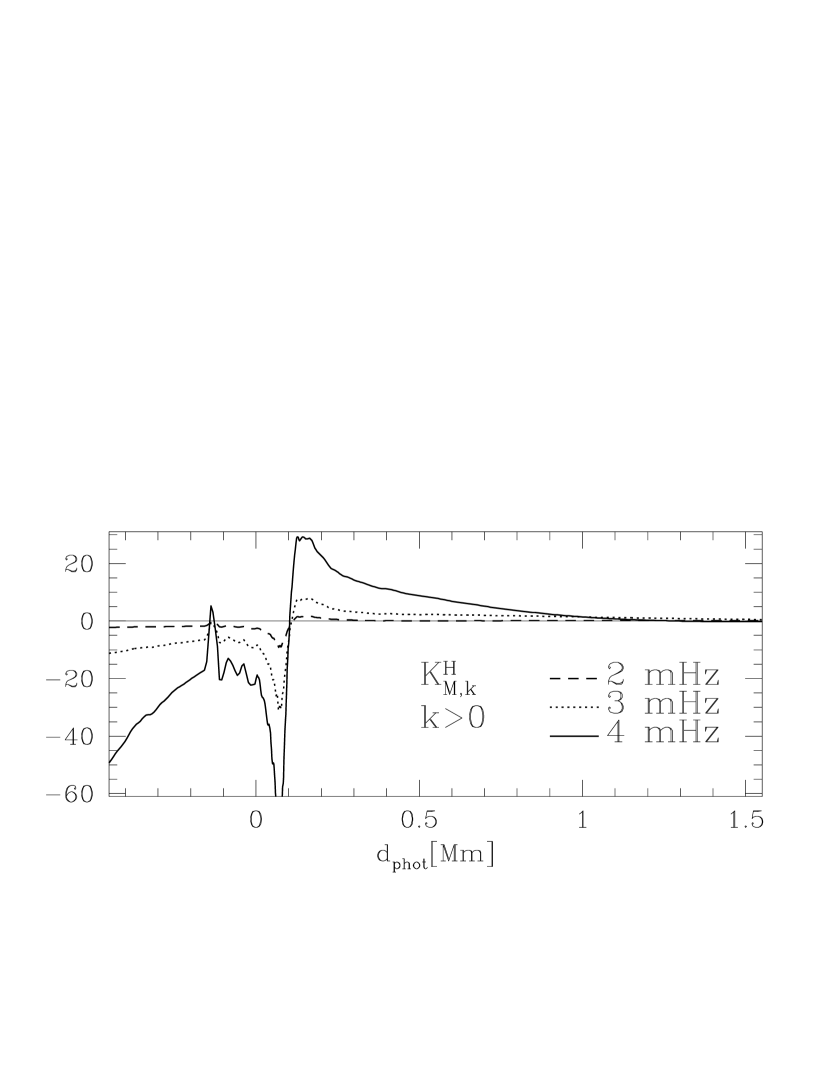
In Fig.1, we show examples of the $K_{v}$ kernels that are important for evaluating the p-mode $\gamma$’s due to the perturbation of the turbulent pressure. Although the general trend is consistent with the asymptotic formulae (eqs. [55] and [58]), there are visible small-scale structures arising from the derivatives of $\Gamma$, which we have ignored in these two asymptotic formulae. The kernels for multiplying the vertical component, have significantly larger absolute values and are negative. Thus, we expect a rise of the $\gamma$’s with a decrease of turbulent velocities. Since the increasing magnetic activity is expected to inhibit turbulence, the trend of the calculated effect in $\gamma$ is consistent with observations.

With the help of Figure 1, we may roughly estimate the required change in the mean turbulent velocity needed to account for the measured $\gamma$’s, under the assumption that this change is the only source of the $\gamma$’s. From numerical simulations, we know (e.g. Abbett et al., 1997) that velocity fluctuations at the level of 1 km/s persist over the whole layer shown in figure, with a maximum of nearly 3 km/s at $d_{\rm phot}\approx 0.1$. The frequency averaged value of $\gamma_{0}\approx 0.3\mu Hz$ (DGS) requires a fraction (0.2 - 0.5) of one percent decrease in the radial component of velocity fluctuations. The largest $\gamma_{k}$ ($k=1$ and 3) require about one percent decrease. Such small changes would not be easy to detect.

Figure 2: Kernels for calculating $\gamma_{v,k}$ for f-modes at three selected $\ell$-values.

Fig. 2 shows that the kernels for the f-modes are very different from those for the p-modes. In this case, the asymptotic expressions for ${\cal R}$ are quite accurate. The kernels scale as $\Lambda/\nu\propto\ell^{1.5}$. All the kernels have similar shapes, and they all negative. The value of the f-mode kernels are comparable to those of the p-modes. The maximum measured values of $\gamma_{0}$ for f-modes are about twice that for p-modes, but the errors are large. The uncertainty for $k>0$ is even higher.

More detailed analyses of the $\gamma_{k}(\nu)$ dependence reflecting the kernels frequency dependence seen in Figs. 1 and 2 are needed to say more about the nature of the required change in the turbulent velocity. However, at this stage we may already conclude that this change must be regarded as important, perhaps the dominant contributor to solar p-mode and f-mode frequency changes over the activity cycle. The sign of the observed changes agrees with the expected inhibiting effect of the field on convection.

7 Frequency change due to varying small-scale, near-surface magnetic field

With the random field being described by a single $P_{2k}$-component (see eq. [35]), the three terms in the integrand of eq. [16] are transformed as follows

$$\overline{|(\mbox{\boldmath{$B$}}\cdot\mbox{\boldmath{$\nabla$}})\mbox{\boldmath{$\xi$}}|^{2}}\rightarrow$$

$$\left[{\cal M}_{k}^{V}(\lambda^{2}+2\Lambda z\lambda+\Lambda{\cal E})+{\cal M}_{k}^{H}{\Lambda\over 2}{\cal E}\right]Q_{k},$$

$$-2\overline{\mbox{\rm div}\mbox{\boldmath{$\xi$}}^{*}\mbox{\boldmath{$B$}}\cdot(\mbox{\boldmath{$B$}}\cdot\mbox{\boldmath{$\nabla$}})\mbox{\boldmath{$\xi$}}}\rightarrow$$

$$-[2{\cal M}_{k}^{V}\lambda(\lambda+\Lambda z)-{\cal M}_{k}^{H}\Lambda z\lambda]Q_{k},$$

and

$${1\over 2}\overline{|\mbox{\boldmath{$B$}}|^{2}}(\Xi+|\mbox{\rm div}\mbox{\boldmath{$\xi$}}|^{2})\rightarrow$$

$$({\cal M}_{k}^{V}+{\cal M}_{k}^{H})[\lambda^{2}+\Lambda(z\lambda+{\cal E})]Q_{k}.$$

The transformations use integration by parts over the surface, our approximations regarding the eigenfunctions, and the angular dependence of the averaged fields. Note that the first term is fully analogous to the integrand in $D_{v}$ that was considered in the previous section.

With the above expression, we get from eq. [16]

$$D_{M,k} = {Q_{k}\over 4\pi}\int drr^{2}\{\delta{\cal M}_{k}^{V}\Lambda(z\lambda+2{\cal E})+$$

$$\delta{\cal M}_{k}^{H}[\lambda^{2}+\Lambda(2z\lambda+1.5{\cal E})]\}.$$

For the spherically symmetric part of $\Delta D_{s}$, we use eq. [41], ignoring here again the temperature and radius changes. This combined with eq. [36], yields

$$\Delta D_{\rm isoth}={1\over 8\pi}\int drr^{2}{\cal D}_{\rm ad}({\cal M}_{0}^{H}-{\cal M_{0}}^{V}).$$ (61)

Using last two expressions in eq. [19], we get

$$(\Delta\omega)_{M,{\rm isoth}} = {1\over 16\pi\omega I}\int drr^{2}({\cal R}_{M,{\rm isoth}}^{V}{\cal M}_{0}^{V}$$ (62)

$$+{\cal R}_{M,{\rm isoth}}^{V}{\cal M}_{0}^{H}),$$

where

$${\cal R}_{M,{\rm isoth}}^{V}=2\Lambda(z\lambda+2{\cal E})-{\cal D}_{\rm isoth}$$

and

$${\cal R}_{M,{\rm isoth}}^{H}=2\lambda^{2}+\Lambda(4z\lambda+3{\cal E})+{\cal D}_{\rm isoth},$$

with ${\cal D}_{s,{\rm isoth}}$ is given in eq. [42]. The complete expressions for the ${\cal R}$’s are in the Appendix (eqs. [A3] and [A4]). The asymptotic expressions for the p-modes are

$${\cal R}_{M,{\rm isoth}}^{V}\approx\left(\Gamma+{\Gamma\over\chi_{\rho}}\right)\lambda^{2}$$

and

$${\cal R}_{M,{\rm isoth}}^{H}\approx\left(2-\Gamma-{\Gamma\over\chi_{\rho}}\right)\lambda^{2}.$$ (63)

The adiabatic kernels, equivalent to those found by GMWK, are obtained by replacing $\chi_{\rho}$ with $\Gamma^{-1}$. In both cases the equations imply that an increase in the vertical component leads to a decrease in the frequencies, while the opposite is true for the horizontal component. The sign of frequency shift due to the horizontal field is opposite to what one might have naively expected because the dominant effect of such field arises through the perturbation of the equilibrium structure (the $D_{s}$ term) and not by the direct effect of the field on oscillations (the $D_{M}$ term). The former term is negative because the horizontal field causes a local expansion, hence an increase of the sound propagation time. The vertical field has an opposite effect. An isotropic (${\cal M}_{0}^{H}=2{\cal M}_{0}^{V}$) field increase implies a net frequency increase but the required increase to account for the observed frequency changes is large.

For the f-modes, the ${\cal D}_{s,{\rm isoth}}$ may be neglected and we have

$${\cal R}_{M,{\rm isoth}}^{V}\approx{\cal R}_{M,{\rm isoth}}^{H}\approx{4\over 3}\Lambda{\cal E}.$$ (64)

Thus, an increase of either component of the magnetic field implies a frequency increase for f-modes.

For $k>0$ we have from eqs. [49] and [36]

$$\Delta D_{s,k} = {Q_{k}\over 8\pi}\int drr^{2}[({\cal D}_{s}^{H}-{\cal D}_{s}^{V}){\cal M}_{k}^{V}$$

$$+{\cal D}_{s}^{V}{\cal M}_{k}^{H})]$$

and

$$(\Delta\omega)_{M,k} = {Q_{k}\over 16\pi\omega I}\int drr^{2}({\cal R}_{M}^{V}{\cal M}_{k}^{V}$$ (65)

$$+{\cal R}_{M}^{H}{\cal M}_{k}^{H}),$$

where

$${\cal R}_{M,k}^{V}={\cal D}_{s}^{H}-{\cal D}_{s}^{V}+2\Lambda(z\lambda+2{\cal E})$$

and

$${\cal R}_{M,k}^{H}={\cal D}_{s}^{V}+2\lambda^{2}+\Lambda(4z\lambda+3{\cal E}).$$

Expressions for ${\cal D}_{s}^{V}$ and ${\cal D}_{s}^{H}$ are given in eqs. [50] and [51], respectively. The complete expressions for the ${\cal R}$’s are in the Appendix (eqs. [A7] and [A8]). Again kernels ${\cal R}_{M,k}$ are the same for all $k>0$. The The asymptotic expressions for p-modes are

$${\cal R}_{M,k}^{V}\approx 4\zeta-\Gamma\lambda^{2},\qquad{\cal R}_{M,k}^{H}\approx-2\zeta+2\lambda^{2}.$$ (66)

For the f-modes, we now have

$${\cal R}_{M,k}^{V}\approx 6\Lambda{\cal E},\qquad{\cal R}_{M,k}^{H}\approx\Lambda{\cal E}.$$ (67)

Now we have for $\gamma$’s

$$\gamma_{M,k} = \int d\left({d_{\rm phot}\over\mbox{ 1 Mm}}\right)\left[K_{M,k}^{V}\left({\delta{\cal M}_{k}^{V}\over\mbox{1 kG}}\right)^{2}\right.$$ (68)

$$\left.+K_{M,k}^{H}\left({\delta{\cal M}_{k}^{H}\over\mbox{1 kG}}\right)^{2}\right]\quad\mbox{$\mu$ Hz},$$

where

$$K_{M,k}^{V,H}=1.06\times 10^{-13}{\mbox{1 mHz}\over\nu}x^{2}{\cal R}_{M,k}^{V,H}.$$

Figure 3: Kernels for calculating centroid frequency shifts due to a small-scale magnetic for p-modes at the three selected frequencies.

Figure 4: The same as Fig.3 but for calculating the even-$a$ part of the frequency splitting

In Figs. 3 and 4, we show kernels for calculating $\gamma_{M}$ according to eq.[68]. Note the strong sensitivity to the frequency, which emphasizes the probing power of the $\gamma(\nu)$ dependence. Further, note that the kernels imply that an increase in the radial field in outer layers will lead to an increase in the mean frequency, while that of the horizontal field has the opposite effect. The growth of the vertical field also leads to an increase of $\gamma$’s at $k>0$, but the effect of the horizontal field growth is impossible to predict as it depends a lot on the depth where it takes place. Also in the case of magnetic fields the kernels for f-modes differ significantly from those for p-modes as we may see comparing Fig. 5 with those in Figs. 3 and 4. For f-modes, the effect of the horizontal components of the field is similar to the vertical ones but smaller.

Figure 5: Kernels for calculating the centroid shifts (upper panel) and splittings due to vertical components of the field for f-mode modes at three selected degrees. The kernels due to the horizontal components have similar shapes but smaller (factor $\approx 3$ at $k=0$ and $\approx 6$ at $k>0$).

Again, we may use the plots shown in these figures to assess the required magnetic field changes needed to account for the measured $\gamma$’s. Let us first consider $\gamma_{0}$. For p-modes, the minimum requirement for the field increase is obtained, if we assume that only radial component increases and it is $\sim 100$ G (DGS). The number rises to above 200 G if we assume an isotropic field increase (GMWK, DGS). This latter value is unacceptably high. Also, there is a higher requirement to account for f-mode $\gamma_{0}$’s. Though the observational accuracy is poorer than in case of p-modes, this may be regarded as a piece of evidence against the direct effect of a changing magnetic field as the sole cause of the frequency changes. Also accounting for the even-$a$ coefficients sets more stringent requirements on the near-surface magnetic field, which may be difficult to reconcile with the measurements.

8 Temperature and radius variation

GMWK were first to considered the role of temperature variations in the p-mode frequency changes. They correctly observed that the temperature decrease at constant pressure results in frequency decrease because the effect of local expansion exceeds that of sound speed increase. However, they excluded the effect of temperature change as a primary source of the measured frequency changes. Here we reconsider the effect using our formulation presented in Section 5.1. With eqs. [20],[19], [41], and [43] we obtain the following expression for the temperature contribution to $\gamma_{0}$.

$$\gamma_{T,0} = \int d\left({d_{\rm phot}\over\mbox{ 1 Mm}}\right)K_{T}$$ (69)

$${\delta T\over T}\quad\mu{\rm Hz},$$

where

$$K_{T}=-0.72{\nu\over\mbox{1 mHz}}\left({c\over\omega r}\right)^{2}x^{4}\tilde{\rho}{\chi_{T}\over\chi_{\rho}}{\cal R}_{T}$$

and

$${\cal R}_{T}=(1+\Gamma_{\rho})\lambda^{2}+2\Lambda z\lambda.$$

For p-modes the first term is dominant in ${\cal R}_{T}$. Except for our taking into account the derivative of $\Gamma$, it is the same as in GMWK. For f-modes the second term is much greater but the entire kernels are much smaller than for p-modes, as we may see in Fig. 6. Thus, we will consider the effect of temperature only for the p-modes. With the plots in the upper panel, we may estimate that the fractional temperature increase in the outer layers at a $10^{-4}$ level implies decrease of $\gamma_{0}$ at a $10^{-1}\mu$Hz level, which is significant. The question arises whether such temperature changes during the solar cycle are feasible.

Figure 6: Kernels for calculating the frequency shifts due to temperature increase for p-modes at the selected frequencies (upper panel) and f-mode modes at the selected degrees (lower panel).

Temperature variation correlated with magnetic variations are expected. However even the sign of it is a matter of debate. Gray & Livingston (1997) put forward evidence that there an increase of $T_{\rm eff}$ between the activity minimum and maximum by some 1.5K, that is $\delta T_{\rm eff}/T_{\rm eff}\approx 2.6\times 10^{-4}$, which would account for the observed variation in the solar constant. Since the optical depth increases with temperature increases, $\delta T$ at $d_{\rm phot}=0$ is somewhat greater than $\delta T_{\rm eff}$. An estimate using the Eddington approximation yields $\delta T(d_{\rm phot})=1.4\delta T_{\rm eff}$. The result of Gray & Livingston is not generally accepted. Spruit(1991) argues that the dominant effect of the magnetic field on temperature is through inhibition of convection and hence it implies cooler layer outer layers at high activity. If this indeed the case, then the induced temperature variation contribute to frequency increase. Spruit (1991) explains the irradiance increase correlated with the activity as a result of an increased corregation of the photosphere.

In a crude manner, the expected temperature change may be linked to the change in the turbulent velocity. In Section 6, we found that $(2-5)\times 10^{-3}$ change in turbulent velocity suffices to explain the maximum value of $\gamma_{0}\approx 0.3\mu$Hz. Our aim is to estimate the values of $\delta T/T$ in the subphotospheric layer extending down to (say) 1 Mm associated with such a change in the velocity. To this aim, we rely on the mixing-length approximation (MLT) and we mimic the inhibiting effect of the field by varying the MLT parameter $\alpha$. While perturbing $\alpha$, we keep both $R$ and entropy constant in the adiabatic part of the convective zone. Adopting $\delta v/v=-3\times 10^{-3}$, we find $\delta T/T=-1\times 10^{-3},-2\times 10^{-4},\mbox{ and}-1\times 10^{-4}$ at $d_{\rm phot}=0$, 0.5, and 1 Mm, respectively. The implied 4 K decrease of $T_{\rm phot}$ between solar minimum and maximum seems unacceptably large. This, however, should not be regarded as a case against changes in turbulent velocities being the primary source of the frequency changes because our treatment of energy transport was very crude indeed. Rather, we want to emphasize here that temperature changes in the subphotospheric layers must be considered as significant contributor to the observed frequency changes over the solar cycle.

The aspherical part of the temperature perturbation is fixed by the condition of mechanical equilibrium. Eq. [29] expresses $\delta_{k}T$ in terms of the expansion coefficients ${\cal V}_{k}$ and ${\cal H}_{k}$, which in turn are linked to the expansion coefficients for turbulent pressure (eq. [34]) and magnetic field (eq. [36]). We may see that any inference on temperature depends on the derivative of the perturbing force, and thus requires a detailed analysis of the $\gamma(\nu)$ dependence. Currently available data are probably not accurate enough for this.

In contrast to the effect temperature, which may only be important for p-modes, the effect of radius perturbation is likely to play a role only in f-mode frequency changes. Considering in eq. [41] only the effect of radius perturbation and adopting the approximation $2\Lambda yz\approx{\ell\cal E}$, which is valid for f-modes, we get from eq. [19]

$$\left({\delta\nu\over\nu}\right)_{r,0}=-{3\ell\over 2\omega^{2}I}\int dI{g\over r}{\delta r\over r}.$$

This expression was used by DGS, who argued that the part of the frequency increase which is proportional to $\nu$ may be explained by the part of $\delta r$ which is common to all modes in the f-mode set. Their set contained modes with $\ell$’s from 137 to 300. The common part must originate below the outer part of the sun sampled by all these modes, that is below radius $r=0.988R_{\odot}$. They argued that its likely cause is an increase in the radial component of the magnetic field by few kG. It is ironic that the best evidence for deep seated magnetic field changes may come from modes which do not directly probe the region where the field is located. Unfortunately, what we get with these modes is only an integral constraint on the field. Of course, it would be advantageous to have a direct probe for the deep seated field.

9 Frequency perturbation due the horizontal field in deep layers

It has been argued (see, e.g., D’Silva & Howard 1993) that a horizontal field of $B\sim 10^{5}$ G is present in the region near the base of the convective envelope. Seismic evidence for the presence of such a field is still controversial.

First, we consider a large-scale toroidal field of the form given in eq. [37], and truncated at $j=2$. The consecutive terms in $D_{M}$(see eq. [16]) are calculated under the same approximation as used in §3. The three integrands become

$$|(\mbox{\boldmath{$B$}}\cdot\mbox{\boldmath{$\nabla$}})\mbox{\boldmath{$\xi$}}|^{2}=Wm^{2}(y^{2}|Y_{\ell}^{m}|^{2}+z^{2}|\mbox{\boldmath{$\nabla$}}_{H}Y_{\ell}^{m}|^{2}),$$

$$-2\mbox{\rm div}\mbox{\boldmath{$\xi$}}^{*}\mbox{\boldmath{$B$}}\cdot(\mbox{\boldmath{$B$}}\cdot\mbox{\boldmath{$\nabla$}})\mbox{\boldmath{$\xi$}}=-2Wm^{2}|Y_{\ell}^{m}|^{2}z\lambda,$$

and

$${1\over 2}|\mbox{\boldmath{$B$}}|^{2}(\Xi+|\mbox{\rm div}\mbox{\boldmath{$\xi$}}|^{2}) = W(1-\mu^{2})|Y_{\ell}^{m}|^{2}$$

$$[\lambda^{2}+\Lambda({\cal E}+z\lambda)],$$

where we denoted

$$W\equiv{3\over 4}B^{1}_{t,2}+{15\over 4}B^{2}_{t,2}\mu^{2}+{3\over 2}\sqrt{5}B^{1}_{t,2}B^{2}_{t,2}\mu.$$

Note that the last term in $W$ cancels out upon integration. Calculating the surface integrals first two terms in $D_{M}$, we rely on the following recursion relation (DG 91).

$$q_{k} = {2k-1\over k(4\Lambda+1-4k^{2})}\{q_{k-1}[2\Lambda-$$

$$(2k-1)^{2}-2m^{2}+q_{k-2}(2k-3)(k-1)\},$$

where

$$q_{k}=\int_{-1}^{1}d\mu\int_{0}^{2\pi}d\phi\mu^{2k}|Y_{\ell}^{m}|^{2}.$$

With this relation, assuming $\Lambda\gg 1$ and using explicit expressions for $P_{2k}$ the surface integral becomes

$$m^{2}\int_{-1}^{1}d\mu\int_{0}^{2\pi}d\phi\mu^{2}|Y_{\ell}^{m}|^{2} \approx$$

$$\Lambda\left({1\over 15}-{2\over 21}Q_{1}-{32\over 105}Q_{2}\right).$$

We could assume $\Lambda\gg 1$ because for low degree modes the third terms dominates. The surface integral in this term is easily expressible in terms of $Q_{1}$ and $Q_{2}$. Combining all the three terms in eq. [16], we obtain

$$D_{M} = {1\over 4\pi}\int drr^{2}\bigg{\{}B_{t,1}^{2}\bigg{[}{1\over 4}(2\lambda^{2}+3\Lambda{\cal E})$$

$$-{Q_{1}\over 2}(\lambda^{2}+3\Lambda{\cal E}-3\Lambda z\lambda)\bigg{]}+B_{t,2}^{2}$$

$$\bigg{[}{1\over 4}(2\lambda^{2}+3\Lambda{\cal E})+{5Q_{1}\over 14}(\lambda^{2}+3\Lambda z\lambda)$$

$$-{2Q_{2}\over 7}(3\lambda^{2}+7\Lambda{\cal E}-5\Lambda z\lambda)\bigg{]}\bigg{\}}$$

We now proceed to calculate the contribution to the centroid frequency changes due to the induced adiabatic pressure change. The adiabatic approximation is now well-justified on the grounds that the layer where the field is expected is located deep enough. Setting $\delta S=0$ in eq. [45] and using eq. [38], to express ${\cal V}_{0}$, we obtain

$$\Delta D_{s,0}={1\over 16\pi}\int drr^{2}{\cal D}_{\rm ad}(B_{t,1}^{2}+B_{t,2}^{2}).$$

Eq. [46] gives an explicit form of ${\cal D}_{s,{\rm ad}}$ in terms of the eigenfunctions.

The corresponding contribution to the splittings is obtained from inserting eqs. [39] and [40] into eq. [49] yields

$$D_{s,k} = {Q_{k}\over 8\pi}\int drr^{2}\bigg{\{}B_{t,1}^{2}\bigg{[}-{1\over 2}({\cal D}_{s}^{V}+)\delta_{k1}\bigg{]}$$

$$2{\cal D}_{s}^{H}+B_{t,2}^{2}\bigg{[}{1\over 14}(5{\cal D}_{s}^{V}-10{\cal D}_{s}^{H})\delta_{k1}$$

$$-{3\over 7}(2{\cal D}_{s}^{V}+3{\cal D}_{s}^{H})\delta_{k2}\bigg{]}\bigg{\}}.$$

Combining all three $D$ integrals into a single expression for the frequency shift due the $j^{\rm th}$-component of the toroidal field, we have

$$(\Delta\omega)_{t,j}={1\over 8\pi I\omega}\sum_{k=0}^{j}Q_{k}\int drr^{2}B_{t,j}^{2}{\cal R}_{t,kj}.$$ (70)

The $j^{\rm th}$ component generates all the $\gamma$’s from $k=0$ up to $j$. From the $D$’s calculated above, we get for the following expressions for the ${\cal R}$’s at $j=1$ and 2

$${\cal R}_{t,01}={\cal R}_{t,02}={1\over 2}{\cal D}_{\rm ad}+\lambda^{2}+{3\over 2}\Lambda{\cal E},$$

$${\cal R}_{t,11}=-{1\over 2}[{\cal D}_{s}^{V}+2{\cal D}_{s}^{H}+2\lambda^{2}+6\Lambda({\cal E}-z\lambda)],$$

$${\cal R}_{t,12}={5\over 14}({\cal D}_{s}^{V}-2{\cal D}_{s}^{H}+2\lambda^{2}+6\Lambda z\lambda)$$

$${\cal R}_{t,22} = -{1\over 7}[6{\cal D}_{s}^{V}+9{\cal D}_{s}^{H}+12\lambda^{2}+$$

$$4\Lambda(7{\cal E}-5z\lambda)]$$

The quantities ${\cal D}_{\rm ad}$, ${\cal D}_{s}^{V}$, and ${\cal D}_{s}^{H}$, are given in eqs. [46], [50] and [51], respectively. In these equations, one may make use of yet another approximation that is valid for p-modes in the acoustic propagation zone and beneath. For solar p-modes (the f-modes are irrelevant here), we have $\lambda\approx-\Lambda\eta z$, where

$$\eta\equiv\left({\omega\over{\cal L}_{\ell}}\right)^{2}={1\over\Lambda}\left({\omega r\over c}\right)^{2}$$

is the square of the ratio of the mode to Lamb frequencies. At the inner turning point, we have $\eta=1$. With the above expression for $\lambda$, we will obtain a more explicit form of the ${\cal R}$’s. The products of the eigenfunctions occurring in the ${\cal R}$’s may now be expressed as follows

$$z\lambda=-\eta{\cal E}^{H},\quad\lambda^{2}=\Lambda\eta^{2}{\cal E}^{H},\quad{\cal E}^{H}\equiv\Lambda z^{2},$$ (71)

$$\zeta={\Lambda\omega^{2}r\over g}yz(2-\eta)={c^{2}\over gr}\Lambda^{2}\eta(2-\eta)yz.$$ (72)

Finally, we assume the ideal gas law, which is a fully adequate approximation in the region considered, to obtain

$${\cal R}_{t,01} = {\cal R}_{t,02}\approx\Lambda\bigg{[}{11\over 12}{\cal E}-\bigg{(}{\eta^{2}\over 3}-2\eta$$

$$+{3\over 5}\bigg{)}{\cal E}^{H}\bigg{]}$$

$${\cal R}_{t,11}\approx-\zeta-\Lambda\left[{\cal E}+\eta\left(5-{2\eta\over 3}\right){\cal E}^{H}\right]$$

$${\cal R}_{t,12}\approx-{15\over 7}\zeta+{5\over 7}\Lambda\left[2{\cal E}+\eta\left({8\over 3}\eta-5\right){\cal E}^{H}\right]$$

$${\cal R}_{t,22}\approx-{6\zeta\over 7}-{\Lambda\over 7}[10{\cal E}-\eta(3\eta+38){\cal E}^{H}]$$

We now rewrite eq. [70] in the following convenient form, specialized for the sun

$$\gamma_{t,k}=\sum_{j\geq k}\int_{0}^{1}dxK_{t,kj}\left({B_{t,j}\over\mbox{1 MG}}\right)^{2}\quad\mbox{$\mu$Hz},$$ (73)

with $x=r/R_{\odot}$

$$K_{t,kj}=1.48\times 10^{-4}{\mbox{1 mHz}\over\nu}x^{2}{\cal R}_{t,k}.$$

Figure 7: Kernels for calculating the values of $\gamma_{t,0}$ according to eq. [73], and arising from dipolar ($j=1$) and quadrupolar ($j=2$) toroidal magnetic fields, for four $\ell=30$ modes of indicated orders $n$ in the zone near the bottom of the convective envelope ($x=r/R_{\odot}=0.71$).

The modes that are most sensitive to the field in the vicinity of the base of the convective envelope are those of moderate degree with turning points located there. This is illustrated in Figs. 7 and 8, where we show the kernels $K_{t,k}(x)$ for three $\ell=30$ modes. The modes have frequencies in the 1.95 to 2.63 mHz range. The lower turning points range, accordingly, from $x=0.742$ to 0.654. The $n$=6 mode, which has its inner turning point at $x=0.721$ that is above the base of the convective zone, probes the field not only within the convective envelope, but also the region immediately beneath, which is below its inner turning point! This latter fact is in contrast to the ray approximation in which this mode would know nothing about the region beneath its inner turning point. The turning of the $n=8$ mode is at $x=0.68$ and this mode is the best probe of the bulk of the overshooting zone that extends down to about 0.70. Similar results would apply for different $\ell$-values, after an appropriate re-scaling of the frequencies so that the $\eta\propto\ell/\nu$ ratio is preserved. We see that the toroidal field increase leads to a corresponding increase in $\gamma_{0}$ and that the effect is mostly of the opposite sign for $k>0$.

Figure 8: The same as Fig.7 but for the even-$a$ splittings ($k>0$).

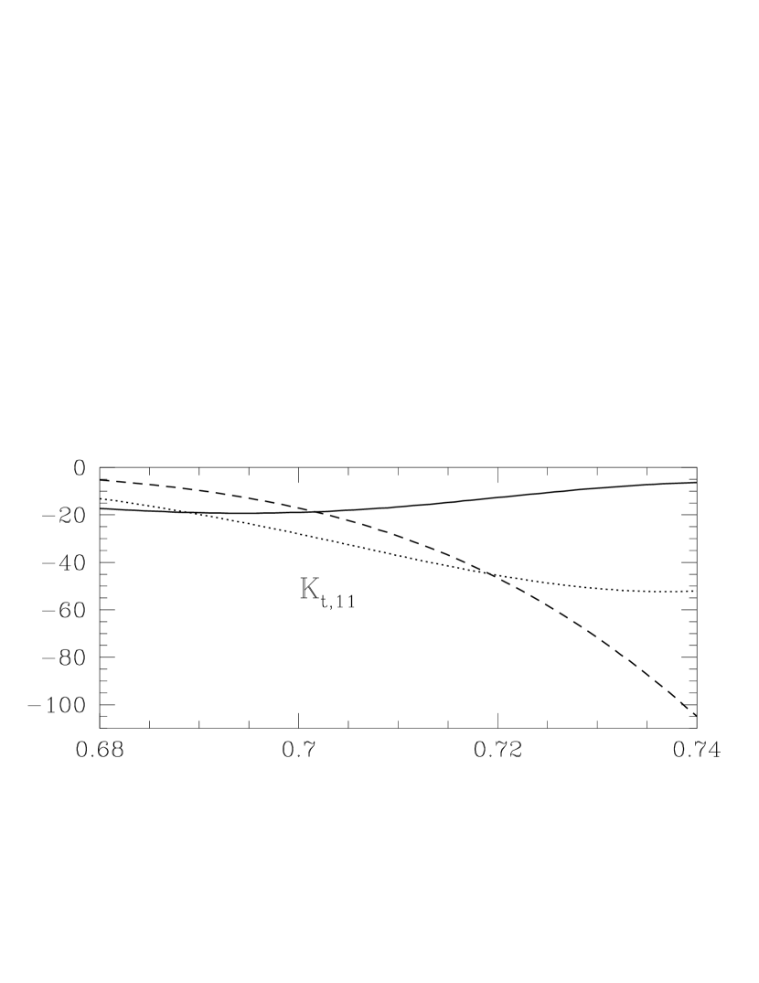
If a toroidal field of 1 MG would prevail in the layer between $x=0.68$ and 0.74, that is over a distance comparable to one pressure scale height, which is about 0.08, then the value of $\gamma_{0}$ would reach up to $0.8\mu$Hz, that of $\gamma_{1}$ would be negative, reaching to -2.6, and that of $\gamma_{2}$ would also be negative reaching $-2.9\mu$Hz. Clearly, such values are very significant and the field would be easily detectable. Detection of the signal corresponding to a putative 0.1 MG field is problematic at present day accuracy. The best chance is to see it is in the even-$a$ coefficients, if indeed the field were dominated by the low-$j$ polynomials. If the 1 MG field were present only within the overshoot zone, extending from (say) x=0.65 to the base of the convective zone, then the corresponding extreme values would be -0.31, -0.95, and -1.1 $\mu$Hz. Thus, somewhat stronger than 0.1 MG fields are required for detection. However, stronger fields may be anticipated in the overshoot layer.

Chou and Serebryanskyi (2002) found evidence for a 0.4-0.7 MG field at the base of the convective envelope from time-distance seismology. Such a field, if it persists over a distance to comparable to that assumed by us, should be detectable by means of global seismology. However, the effort made so far did not result in the detection of a significant signal (Basu, 2002).

Figure 9: Kernels for calculating the $\gamma$’s arising from small-scale horizontal magnetic field near the base of the solar convective zone.

It is possible that the magnetic field in the deep part of the convection envelope, and in the overshoot zone forms azimuthal ropes, and thus is better represented as a small-scale field with its mean value being a slowly varying function of latitude. In this case, the frequency perturbation is described by the adiabatic version of eqs. [62], at $k=0$, and by [65], at $k>0$, with only the horizontal components included. For the $\gamma$’s, we use an expression that is similar to that given in eq. [68]

$$\gamma_{k}^{H}=\int_{0}^{1}dxK_{k}^{H}\left({B_{t,j}\over\mbox{1 MG}}\right)^{2}\quad\mbox{$\mu$Hz},$$ (74)

with $x=r/R_{\odot}$

$$K_{k}^{H}=1.48\times 10^{-4}{\mbox{1 mHz}\over\nu}x^{2}{\cal R}^{H}_{M,k}.$$

With the approximation for the eigenfunctions, which is valid for p-modes in the zone considered as given in Eqs. [71] and [72], we have

$${\cal R}^{H}_{M,0}\approx\Lambda\left[{11\over 5}{\cal E}-\left({2\over 3}\eta^{2}+{6\over 5}\right){\cal E}^{H}\right]$$

$${\cal R}^{H}_{M,k}\approx\Lambda\left[3{\cal E}+2\eta(\eta-2){\cal E}^{H}\right]-2\zeta.$$

Both kernels change sign in the region of interest. In Fig. 9, we show examples of the kernels for the same modes and in the same layer, as in Fig. 8. Differences between the figures are apparent. Note in particular, the sign changes within the layer. With a 1MG field in the layer, we get $\gamma_{0}$ of about 0.8 $\mu$Hz for the $n=8$ and 10 modes. The absolute values at $k>0$ are somewhat lower. So that a 0.4-0.7 MG field should be easily detectable in the frequency shifts. The expected signal in the even-$a$’s would be somewhat weaker, but should also be detectable.

10 Conclusions

We surveyed various effects that may explain the increase of the mean frequencies of solar oscillations and the changes in the fine structure of the multiplets correlated with the rise of activity. Beyond any doubt is the fact that the seismic changes reflect temporal and longitudinal evolution of the sun’s activity and that the main part of these changes has its source close to photosphere, perhaps within 1 to 1.5 Mm. The question that remains to be answered is how the changes are related to magnetic field variations and associated variation of the velocity field and the temperature in the atmosphere, and in the subphotospheric layers. The answer is important because only after we know it, we will be able to make a full use of seismic data as a probe of the large-scale variability of the sun over its activity cycle.

Another open question is whether current frequency data reveal changes in the deep interior. Assessing the intensity of the magnetic field in the lower convective envelope and in the outer radiative interior, just beneath, would be of great importance for understanding the physics of magnetic activity.

With these questions in mind, we developed integral formulae expressing shifts in oscillation frequencies in terms of changes in magnetic and velocity fields and temperature. We made certain approximations, which are well-justified both for solar p- and f-modes. Small scale-fields were represented by the square-averaged values of vertical and horizontal components. These values were expressed in terms of the Legendre-polynomial series. We showed the coefficients at $P_{2k}$ in these series contribute only to $a_{2k}$ coefficients of the frequency splitting. The connecting expressions were given in the form of integrals over the depth with explicit expressions for the kernels. We also provided kernels linking the mean frequency shifts and the $a_{2k}$ coefficients to a low-order expansion of a putative large-scale toroidal field near the base of the convective envelope.

Plots of the kernels allowed us to make a simple assessment of the changes needed to explain the measured shifts. We found that the increase of the mean frequencies and the changes in $a_{2k}$-coefficients are most easily explained in terms of a decrease of turbulent velocities associated with the increase of the magnetic field with growing activity. The required decrease in the turbulent velocity needed to explain the data constitutes only a fraction of a percent. A decrease in turbulent velocity is expected to result in a temperature decrease in outer layers of the sun. Our estimate showed that the resulting temperature decrease should give a significant contribution to the mean frequency increase, which reduces requirement on the size of the decrease of the turbulent velocity. Accounting for the seismic changes by the sole direct effect magnetic field is more difficult. An increase of the surface-averaged r.m.s. value of the vertical field component by about 0.1 kG between the minimum and maximum of the activity would be needed to account for the mean frequency increase of the p-modes. The measured changes in the even $a$ coefficient for p-mode require about twice as large field increase at most active latitudes. Also a larger field seems to be needed to account for the systematic increase of the f-mode frequencies.

Considering the influence of the field near the base of the convective envelope, we found that there is a chance for detecting such a field directly from the frequency data. Evidence, from time-distance seismology, for the presence there of the $(0.4-0.7)$ MG field was recently put forward by Chou & Serebryanskyi (2002). We showed that such a field, if extends over a layer of thickness comparable with one pressure distance scale, should be detectable also by means of global seismology.

11 Kernels for the $\gamma$’s

Here we summarize the expressions for the kernels for evaluating the $\gamma$’s due to small-scale velocity and magnetic fields. We begin by recalling the definition of the radial eigenfunctions:

$$\mbox{\boldmath{$\xi$}}=r[y(r)\mbox{\boldmath{$e$}}_{r}+z(r)\mbox{\boldmath{$\nabla$}}_{H}]Y_{\ell}^{m}(\theta,\phi)\exp(-{\rm i}\omega t).$$

We also define

$$\lambda=y{gr\over c^{2}}-z{\omega^{2}r^{2}\over c^{2}}$$

and

$${\cal E}=y^{2}+\Lambda z^{2}.$$

The kernels for centroid shifts ($\gamma_{0}$) due to turbulent velocity are

$${\cal R}_{v,{\rm isoth}}^{V}={\cal D}_{\rm isoth}-(\lambda^{2}+2\Lambda z\lambda+\Lambda{\cal E})$$

$${\cal R}_{v,0}^{H}=-{\Lambda\over 2}{\cal E}.$$

and those due to a small-scale magnetic fields are

$${\cal R}_{M,{\rm isoth}}^{V}=2\Lambda(z\lambda+2{\cal E})-{\cal D}_{\rm isoth}$$

$${\cal R}_{M,{\rm isoth}}^{H}=2\lambda^{2}+\Lambda(4z\lambda+3{\cal E})+{\cal D}_{\rm isoth}.$$

where

$${\cal D}_{\rm isoth} = -\Gamma\bigg{[}\bigg{(}1+\Gamma_{p}+{1+\Gamma_{\rho}\over\chi_{\rho}}\bigg{)}\lambda^{2}$$

$$+{2\Lambda z\lambda\over\chi_{\rho}}\bigg{]}$$

The kernels for the even-$a$ coefficients ($\gamma_{k}$, $k>0$) due to turbulent velocity are

$${\cal R}_{v,k}^{V}=-(2\zeta-\psi+\lambda^{2}+2\Lambda z\lambda+\Lambda{\cal E}),$$

$${\cal R}_{v,k}^{H}=\zeta-{1\over 2}[\psi-\Gamma(1+\Gamma_{p})\lambda^{2}+2\Lambda z\lambda+3\Lambda{\cal E}].$$

and those due small-scale magnetic fields

$${\cal R}_{M,k}^{V}=4\zeta-2\psi-\Gamma(1+\Gamma_{p})\lambda^{2}+2\Lambda{\cal E},$$

$${\cal R}_{M,k}^{H}=-2\zeta+\psi+2\lambda^{2},$$

where

$$\zeta={\omega^{2}r\over g}(y\lambda+2\Lambda zy)$$

and

$$\psi \equiv \Gamma_{\rho}\bigg{[}\bigg{(}2-\Gamma{d\ln c^{2}\over d\ln p}\bigg{)}\lambda^{2}+2\lambda\bigg{(}\Lambda z$$

$$-{\omega^{2}r\over g}y\bigg{)}\bigg{]}-\Gamma{d\Gamma_{\rho}\over d\ln p}\lambda^{2}.$$

References

- Abbet (1997) Abbet, W.B, Beaver, M., Davids, B., Georgobiani, D., Rathbin, P., & Stein, R.F. 1997, ApJ, 480, 395
- Basu (2002) Basu, S. 2002, in From Solar Min to Max: Half a Solar Cycle with SOHO, Proceedings of the SOHO 11 Symposium, ed. A. Wilson, ESA SP-508, p. 6
- Chou (2002) Chou, D.-Y. &Serebryanskiy, 2002, ApJ, 578, L157
- D’Silva & Choudhuri (1993) D’Silva ,S.& Choudhuri , A.R. 1993, A&A, 272, 621
- Dewar (1970) Dewar, R. L. 1970, Phys. Fluids, 13, 2710
- Dziembowski & Goode (1991) Dziembowski, W.A. & Goode, P. R. 1991, ApJ, 376, 782
- Dziembowski & Goode (1992) Dziembowski, W. A. & Goode, P. R. 1992, ApJ, 394, 670
- Dziembowski & Goode (2002) Dziembowski, W. A. & Goode, P. R. 2002, in Radial and non-radial pulsations as probes of stellar physics, Proceedings of IAU Symp. 185, eds. C. Aerts & T. Bedding, PASP, p.476
- Goldreich et al. (1991) Goldreich, P., Murray, N., Willette, G., & Kumar, P. 1991, ApJ, 370,752
- Goode & Dziembowski (2002) Goode, P. R. & Dziembowski, W. A. 2002, in From Solar Min to Max: Half a Solar Cycle with SOHO, Proceedings of the SOHO 11 Symposium, ed. A. Wilson, ESA SP-508, p. 15
- Gough & Thompson (1990) Gough, D.O., Thompson, M.J. 1990, MNRAS, 242, 25
- Gray& Livingston (1997) Gray, D.F. & Livingston, W.C. 1997, ApJ, 474, 802
- Kuhn (2000) Kuhn, J.R. 2000, Space Sci.Rev., 94, 177
- Lynden-Bell & Ostriker (1967) Lynden-Bell, D. & Ostriker, J. P. 1967, MNRAS, 136, 293
- Ritzwoller & Lavely (1991) Ritzwoller, M. H. & Lavely, E. M. 1991, ApJ, 369, 557
- Schou et al. (1994) Schou, J., Christensen-Dalsgaard, J. & Thompson, M. J. 1994, ApJ, 433, 289
- Spruit (1991) Spruit, H.C. 1991 in The Sun The Time, eds. Sonett, C.P., Giampappa, M.P., & Matthews, M.S., University of Arizona Press, p. 118