Global, Exact Cosmic Microwave Background Data Analysis Using Gibbs Sampling

Abstract

We describe an efficient and exact method that enables global Bayesian analysis of cosmic microwave background (CMB) data. The method reveals the joint posterior density (or likelihood for flat priors) of the power spectrum $C_{\ell}$ and the CMB signal. Foregrounds and instrumental parameters can be simultaneously inferred from the data. The method allows the specification of a wide range of foreground priors. We explicitly show how to propagate the non-Gaussian dependency structure of the $C_{\ell}$ posterior through to the posterior density of the parameters. If desired, the analysis can be coupled to theoretical (cosmological) priors and can yield the posterior density of cosmological parameter estimates directly from the time-ordered data. The method does not hinge on special assumptions about the survey geometry or noise properties, etc. It is based on a Monte Carlo approach and hence parallelizes trivially. No trace or determinant evaluations are necessary. The feasibility of this approach rests on the ability to solve the systems of linear equations which arise. These are of the same size and computational complexity as the map-making equations. We describe a pre-conditioned conjugate gradient technique that solves this problem and demonstrate in a numerical example that the computational time required for each Monte Carlo sample scales as $n_{p}^{3/2}$ with the number of pixels $n_{p}$. We test our method using the COBE-DMR data and explore the non-Gaussian joint posterior density of the COBE-DMR $C_{\ell}$ in several projections.

I Introduction

The observation and analysis of cosmic microwave background (CMB) anisotropies have attracted a great deal of attention in recent years due to their unique relevance for cosmological theory (see review for a recent review). A slew of observational results have been published during the last two yearscmbobs . These were obtained from maps of the microwave sky at ever increasing sensitivity and resolution. Since the recent release of the first year WMAP data, an all-sky microwave survey has been available down to angular scales of 12 minutes of arc mapresults . By the end of the decade the Planck satellite is expected to generate 1 Terabyte of high resolution, high sensitivity all-sky data.

The basic assumption is that the CMB anisotropy signal and the instrumental noise are Gaussian and that the signal statistics are isotropic on the sky. Contact between theory and observation is then best made by extracting the angular power spectrum $C_{\ell}$ from the dataBondEfstathiou ; Tegmark ; BJK . Methods for efficiently estimating the power spectrum have been investigated since the computational unfeasiblity of using the brute-force approach was realized Gorski ; BCJK ; Borrill . This effort has yielded two classes of methods: exact methods, applicable only to two narrowly defined classes of observational strategies OSH ; WH , and approximate but more broadly applicable methods pseudocl ; MASTER ; szapudi .

We will describe here a solution to the problem of inference from microwave background data which combines the advantages of exact methods with the practicality of the approximate methods. The computational cost of our method scales like the best approximate method for the same experiment, albeit with a larger pre-factor. Power spectrum estimates and any desired characterization of the (multivariate) statistical uncertainty in the estimates can be computed free from any approximations in the estimator which could lead to sub-optimality or biases.

The solution we propose is to sample the power spectrum (as well as other desired quantities, such as the underlying CMB signal, foregrounds or the noise properties of the instrument) directly from the joint likelihood (or posterior) density given the data. We can efficiently sample from this multi-million dimensional density using the Gibbs sampler. This approach obviates the need to evaluate the likelihood or its derivatives in order to analyze CMB data.

Our approach shares certain algorithmic features with the approach independently discovered in Jewell which describes a maximum likelihood estimator of the power spectrum using Bayesian Monte Carlo methods. However, our goal from the outset was to design a method that allows a full exploration of the multivariate probability density of the power spectrum and the parameter estimates, given the data.

Our method seamlessly integrates with parameter estimation without recourse to semi-analytic Gaussian, offset log-normal RadPack , $\chi^{2}$ Bartlett or hybrid WMAPverde approximation schemes. If desired, theoretical priors can be applied in the analysis by restricting the space of power spectra to those which arise from a physical model of the CMB anisotropy.

By design, the sample of power spectra and reconstructed sky maps will reflect the statistical uncertainty given the data through the full non-Gaussian statistical dependence structure of the $C_{\ell}$ estimates. This information can be propagated losslessly to the cosmological parameter estimates.

One aspect of our method which is of general interest in astrophysics beyond CMB analysis is that it generalizes the results on globally optimal interpolation, filtering and reconstruction of noisy and censored data sets in rybickipress to self-consistently include inference of the signal covariance structure. This defines a generalized Wiener filter that does not need a priori specification of the signal covariance. A byproduct of our method is a prescription for “unbiasing” the Wiener filter which clearly reveals the tight relation between Wiener filtering and power spectrum estimation.

Our methods differ from traditional methods of CMB analysis in a fundamental aspect. Traditional methods consider the analysis task as a set of steps, each of which arrives at intermediate outputs which are then fed as inputs to the next step in the pipeline. Our approach is a truly global analysis, in the sense that the statistics of all the science products are computed jointly, respecting and exploiting the full statistical dependence structure between the various components.

In summary, our method is a Monte Carlo technique which samples power spectra and other science products from their exact, multivariate a posteriori probability density, and which does so without explicitly evaluating it. The result is a detailed characterization of the statistics of the CMB signal on the sky, reconstructed foregrounds, the CMB power spectrum, and the cosmological parameters inferred from it with a cost which is proportional to the cost of a least squares map-making algorithm for the same set of observations.

In section II we introduce notation and a general statistical model of CMB observations. Our method is described in detail in section III. In section IV we comment on the perspective our Bayesian approach offers on cosmic variance. We discuss the numerical and computational techniques used to implement our method in section V and apply it to the COBE-DMR data in section VI. We reflect on where we stand and conclude with comments on further work to be done in section VII.

II Model and Notation

We begin by defining our model of CMB observations and introduce our notation. We imagine that the actual CMB sky $s$ is observed with some optical system and according to some observing strategy encoded in a pointing matrix $A$, which maps the signal on the sky into a collection of $n_{o}$ time-ordered observations of the sky. This results in the “raw” data $d$, represented by a vector with $n_{o}$ elements (an $n_{o}$–vector). Our model of this process is encoded in the model equation

$$d=A(s+f)+n^{tod},$$ (1)

where $n^{tod}$ is a realization of Gaussian instrumental noise added to the data and $f=\sum_{i}f_{i}$ is the sum of a collection of foregrounds (assumed spatially varying and constant in time). We represent maps on the sky with $n_{p}$ resolution elements (pixels) as $n_{p}$–vectors. Note that while we do not explicitly consider multi-channel data, the model is easily generalized to that case by adding a frequency index to $d$, $A$, $n^{tod}$ and $f$.

The “map” vector $m$ is the least squares estimate of the signal $s+f$ from $d$. Because we assume Gaussian noise with zero mean this is also the maximum likelihood estimate (or maximum a posteriori estimate assuming a flat prior). It can be found as the solution of the normal equation

$$A^{T}N_{tod}^{-1}Am=A^{T}N_{tod}^{-1}d.$$ (2)

Here the matrix $N_{tod}$ is the covariance matrix of the noise in the time ordered data space $N_{tod}=\langle n^{tod}n^{tod\;T}\rangle$. Then $m=s+f+n$ where $n$ describes the residual noise on the map estimate with covariance matrix $N=\langle nn^{T}\rangle=(A^{T}N_{tod}^{-1}A)^{-1}$.

The cosmological model specifies the signal covariance matrix $S$. For isotropic theories $S$ is diagonal in the spherical harmonic basis, with the special form $S_{\ell m\ell^{\prime}m^{\prime}}=C_{\ell}\delta_{\ell\ell^{\prime}}\delta_{mm^{\prime}}$.

In keeping with the majority of the literature in the field, we restrict our discussion to theories which predict a Gaussian CMB signal $s$. It will be convenient to abbreviate Gaussian multivariate densities as

$$G(m,C)\equiv\frac{1}{\sqrt{|2\pi C|}}\exp\left(\frac{1}{2}m^{T}C^{-1}m\right).$$ (3)

III Method

III.1 Overview

For a cleaner exposition of the method, we will ignore the foregrounds $f$ for now and return to their inclusion later. We are trying to explore the a posteriori density

$$P(C_{\ell}|m)\propto G(m,S(C_{\ell})+N)P(C_{\ell})$$ (4)

where $P(C_{\ell})$ is the density encoding prior information on the $C_{\ell}$. Up to normalization this can be obtained by marginalizing the joint density

$$P(C_{\ell},s,m)=P(m|s)P(s|C_{\ell})P(C_{\ell})$$ (5)

over the signal $s$. Setting $P(C_{\ell})=const$ makes this analysis equivalent to an exact frequentist likelihood analysis. We will discuss other choices of prior later.

Traditionally, the approach to exploring the a posteriori density has been to define an estimator, such as the least squares quadratic (LSQ) estimator Tegmark or the maximum likelihood (ML) estimator BJK . Then some measure of uncertainty in the values of this estimator was defined, for instance by approximating the shape of $P(C_{\ell}|m)$ around the maximum by a multivariate Gaussian and evaluating elements of the curvature matrix at the extremum.

Evaluating the LSQ or ML estimators is a very costly operation, taking $O(n_{p}^{3})$ operations. In general, evaluating the curvature matrix is even more costly because it has $O(n_{p})$ elements each of which requires $O(n_{p}^{3})$ operations, making the overall operation count of order $O(n_{p}^{4})$. In addition a Gaussian approximation fails at low $\ell$ where the small number of degrees of freedom makes the posterior significantly non-Gaussian, and also at high $\ell$ in the regime of small signal-to-noise ($S/N\lesssim 1$).

Instead, we propose to sample parameter values $C_{\ell}$ from the posterior directly. There is no known way to directly sample from Eq.4, but if a way can be found to sample $s$ and $C_{\ell}$ from the joint distribution Eq. (5) then the $C_{\ell}$ taken by themselves are exact samples from the marginalized distribution.

At first, sampling from the joint distribution seems even less feasible. But powerful theorems can be proved tanner that show that if it is possible to sample from the conditional distributions $P(s|C_{\ell},m)$ and $P(C_{\ell}|s,m)\propto P(C_{\ell}|s)$ then one can sample from the joint distribution in an iterative fashion. Begin with some starting guess $C_{\ell}^{0}$. Then iterate the following equations

$$s^{i+1}\leftarrow P(s|C_{\ell}^{i},m)$$ (6)

$$C_{\ell}^{i+1}\leftarrow P(C_{\ell}|s^{i+1})$$ (7)

then after some “burn-in” the $(C_{\ell}^{i},s^{i})$ converge to being samples from the joint distribution Eq. (5). This technique of sampling from the joint distribution is called the Gibbs sampler.

III.2 Sampling Techniques

To implement these ideas one needs the forms of the conditional densities and recipes for sampling from these distributions. These follow now.

The conditional density of the signal given the most recent $C_{\ell}$ sample is just a multivariate Gaussian

$$P(s|C_{\ell}^{i},m)\propto G\left(S^{i}(S^{i}+N)^{-1}m,((S^{i})^{-1}+N^{-1})^{-1}\right),$$ (8)

where $S^{i}\equiv S(C_{\ell}^{i})$. This will be recognized as the posterior density of the Wiener Filter given the most recent power spectrum estimate.

The density for the power spectrum coefficients $C_{\ell}$ factorizes due to the special form of $S$.

$$P(C_{\ell}|s^{i})\propto P(C_{\ell})\prod_{l}\frac{1}{\sqrt{C_{\ell}^{2\ell+1}}}\exp\left(-\frac{1}{2C_{\ell}}\sum_{m=-l}^{+l}|s^{i}_{\ell m}|^{2}\right)$$ (9)

The $s^{i}_{\ell m}$ are the spherical harmonic coefficients of $s^{i}$. This density is known as the inverse Gamma distribution of order $2\ell-1$. This result has interesting implications for cosmic variance in this Bayesian framework, which we will discuss below.

To sample from Eq. (8) we need to generate a Gaussian variate with the given mean and covariance. A numerically convenient choice (see section V) of the equation for the mean $x$ is

$$(1+S^{i\;\frac{1}{2}}N^{-1}S^{i\;\frac{1}{2}})S^{i\;-\frac{1}{2}}x=S^{i\;\frac{1}{2}}N^{-1}m.$$ (10)

In fact it is easier to solve for $z=S^{i\;-\frac{1}{2}}x$ and to then solve for x trivially. Note from its definition above that $N^{-1}x$ is easier to compute than $Nx$. If $N_{tod}$ is circulant (stationary noise) or block-circulant (a popular choice for non-stationary noise), $N_{tod}^{-1}x$ can be computed using FFTs. If $N$ is diagonal to very good accuracy then computing $N^{-1}$ easy. We will drop the $i$ superscript in what follows.

We chose to write the equation in terms of the map made from the data. It easy to see from Eq. (2) and from $N=(A^{T}N_{tod}^{-1}A)^{-1}$ that writing Eq. (10) in terms of the TOD saves some computations: $N^{-1}m=A^{T}N_{tod}^{-1}d$. This replacement can be made throughout in the equations that follow in the remainder of this paper.

Then we need to add a fluctuation term to this mean to get a random variate. This is non-trivial, because we need to simulate a map with covariance $(S^{-1}+N^{-1})^{-1}$ without being able to compute square roots of this matrix. We can, however, compute the square root of $S$ because it is diagonal in spherical harmonic space and we can compute $N^{-\frac{1}{2}}\equiv A^{T}N_{tod}^{\frac{1}{2}}$ by using FFTs on the time-ordered data. This leads to the following solution: generate two p-vectors $\xi$ and $\chi$ of independent Gaussian random variates, with zero mean and unit variance (these are called normal variates). Then solve the linear set of equations

$$\left(1+S^{\frac{1}{2}}N^{-1}S^{\frac{1}{2}}\right)S^{-\frac{1}{2}}y=\xi+S^{\frac{1}{2}}N^{-\frac{1}{2}}\chi$$ (11)

for y. It is easy to verify that this does give the right covariance by computing $\langle yy^{T}\rangle$. The final result is then

$$s^{i+1}=x+y,$$ (12)

where we have re-introduced the superscript.

Note that each $s$ is a perfect pure signal sky (up to the assumed band-limit) with covariance $S$. While $x$ is the Wiener filter, whose power spectrum would be a biased estimator of the $C_{\ell}$, $s$ is “unbiased”. The addition of the fluctuating term $y$ has replaced filtered noise fluctuations with synthetic signal fluctuations.

Drawing the $C_{\ell}^{i+1}$ from the inverse Gamma distribution, Eq. (9), is very simple. For each $\ell$, compute $\sigma_{\ell}=\sum_{m=-\ell}^{+\ell}|s^{i}_{\ell m}|^{2}$ and generate a $(2\ell-1)$-vector $\rho_{\ell}$ of Gaussian random variates with zero mean and unit variance. Then

$$C_{\ell}^{i+1}=\frac{\sigma_{\ell}}{|\rho_{\ell}|^{2}},$$ (13)

where the denominator is the square norm of $\rho_{\ell}$.

III.3 Foregrounds

Traditionally, regions on the sky are excised if the residual error after foreground subtraction is large. However, modeling the signal on the remainder of the sky after foreground cuts complicates the structure of the signal covariance matrix $S$. Instead, we choose to model foregrounds as an additional component in the model equation, as shown in Eq. (1). Then the joint density in Eq. (5) becomes

$$P(C_{\ell},s,\{f_{j}\},d)=P(d|s,\{f_{j}\})P(s|C_{\ell})P(C_{\ell})\prod_{k}P(f_{k})$$ (14)

where each $P(f_{k})$ contains prior information about the $k$th foreground.

Following the Gibbs sampler approach we draw from the foreground components given the data. We group different logically separate foregrounds by adding in additional steps in the sampling chain

$${\rm~{}for~{}every~{}}j:~{}f_{j}^{i+1} \leftarrow P(f_{j}|C_{\ell}^{i},s^{i},\{f_{k<j}\}^{i+1},\{f_{k>j}\}^{i})$$

$$s^{i+1} \leftarrow P(s|C_{\ell}^{i},\{f_{j}\}^{i+1})$$ (15)

$$C_{\ell}^{i+1} \leftarrow P(C_{\ell}|s^{i+1})$$

Where appropriate, different foreground components may be grouped together into one $f_{j}$. The algorithm to sample from the conditional foreground densities is analogous to the signal sampling algorithm described in the previous subsection. We will return to algorithmic issues after discussing the foreground prior $\prod_{j}P(f_{j})$.

How do we specify the foreground prior? For instance, we might want to be completely insensitive to certain foreground terms $\{f_{i}\}$. This would mean setting $P(f)=G(f,FF^{T})$, where $FF^{T}\equiv\sigma_{f}^{2}\sum_{i}f_{i}f_{i}^{T}$ and each vector $f_{i}$ represents a foreground contribution we would like to project out. The matrix $F$ is just constructed by columns from the $f_{i}$. The variance $\sigma_{f}^{2}$ is numerically “infinite”, i.e. large compared to any other noise source. This specifies maximal ignorance about the amplitude of this foreground component. As an example, $f_{i}$ could be the monopole and the three dipole components. Or, if the foreground contribution in a pixel $j$ was completely unknown, the $f_{i}=1_{j}$ where $1_{j}$ is the vector representing the map which is zero everywhere except in the pixel $j$. Essentially any spatial template to which we want the power spectrum estimation to be insensitive can be added in here, and they can be grouped in computationally convenient ways in Eq. (15).

It is important to note that even though we may have specified “infinite” variance in our prior, the foreground samples produced will be constrained by the data and hence will be informative about the level of the foreground contribution supported by the data. For example, the sample of the three dipole components generated during the iteration of Eq. (15) in the example above would be informative about the direction and amplitude of the CMB dipole, and could be used to calibrate the experiment.

Different choices for the foreground prior $P(f)$ are possible. It could include information on foreground templates as well as a specification of our uncertainty in these templates. For example if the template is $\bar{f}$ and our uncertainty could be described by a Gaussian centered on $\bar{f}$ with covariance $FF^{T}$ then $P(f)=G(f-\bar{f},FF^{T})$. One way to specify $\bar{f}$ and $FF^{T}$ would be to simulate a set of possible theoretical foreground models $f_{i}$ with weights $w_{i}$, such that $\sum w_{i}=1$, and to then set $\bar{f}=\sum w_{i}f_{i}$ and $FF^{T}\equiv\sum_{i}w_{i}(f_{i}-\bar{f})(f_{i}-\bar{f})^{T}$.

Note that the assumption of a Gaussian prior $P(f)$ only assumes that our ignorance of the foreground contribution can be expressed through a Gaussian covariance structure—the foregrounds are not assumed to have Gaussian statistics. Non-Gaussianity can be explicitly assumed by choosing a non-Gaussian template $\bar{f}$. For the case of multi-frequency data, $P(f)$ could encode what is known about the dependence of certain physical foreground components on the frequency.

Returning to the mechanics of sampling Eq. (15) we write ${\cal F}_{j}=F_{j}F^{T}_{j}$, and solve at the $j$th step

$$({\cal F}_{j}+{\cal F}_{j}N^{-1}{\cal F}_{j})x_{j}=\bar{f}_{j}+{\cal F}_{j}N^{-1}(m-s-\sum_{k\neq j}f_{j}),$$ (16)

and

$$\left({\cal F}_{j}+{\cal F}_{j}N^{-1}{\cal F}_{j}\right)y_{j}=F_{j}\xi+{\cal F}_{j}N^{-\frac{1}{2}}\chi.$$ (17)

Then $f_{j}={\cal F}_{j}(x_{j}+y_{j})$. Since ${\cal F}_{j}$ may not be full rank in $n_{p}$ dimensions, the equations here may be understood as shorthand for the projected equations in the subspace on which ${\cal F}_{j}$ has full rank.

Note that when foregrounds are considered, the $m$ on the right hand side of Eq. (10) has to be replaced with $(m-\sum_{j}f_{j})$.

In special cases it may be desirable to perform the marginalization over $f$ analytically. Appendix A gives techniques for doing so.

III.4 Noise model

It is straightforward to extend our methods to include estimation of the noise covariance from the data themselves. In the case that $N_{tod}$ is non-stationary and block-diagonal with circulant blocks (the standard assumption in CMB analysis), we can easily add a sampling step symbolically written as

$$N_{j}^{i+1}\leftarrow P(N|\{N_{k\neq j}\}^{i},s,C_{\ell},\{f_{j}\})=P(N|s,\{f_{j}\}).$$ (18)

The second equality expresses two facts: (1) for a block diagonal noise matrix the conditional density of one block does not depend on the other blocks and (2) $N$ is conditionally independent of the $C_{\ell}$ given $s$; that is given $s$ the $C_{\ell}$ do not add more information about the $N$.

In practice, the noise model would assume smoothness of the noise power spectra. If we write $N_{jk}$ for the $k$th band power spectral coefficient of the $j$th block of the noise covariance of the TOD simply involves computing the FFT of the $j$th segment of $d-A(s+\sum f)$, adding the power in bands of width $d$ and then sampling $N_{jk}$ from the inverse Gamma distributions of order $d-2$.

More general noise models can be implemented. We will explore the effect of more sophisticated modeling of non-stationary noise in future work.

III.5 Parameter estimation

Currently power spectrum estimation algorithms rely on approximate representations of the posterior density $P(C_{\ell}|d)$ , for example in terms of multivariate Gaussian, shifted log-normal or hybrid representations. These approximations have to be fitted to sets of Monte Carlo simulations WMAPverde . Since they take simple analytical forms they can only be expected to be accurate near the peak of the posterior density. In order to faithfully propagate all the information in the $C_{\ell}$ estimates through to the parameter estimation step, efficient ways must be found to accurately represent and communicate $P(C_{\ell}|d)$.

The Bayesian estimation technique described in this paper provides a natural answer to this problem. The method generates a set of samples from $P(C_{\ell}|d)$ which can simply be published electronically. Meaningful summaries of the properties of $P(C_{\ell}|d)$ can all be calculated arbitrarily exactly, given a sufficient number of samples.

The disadvantage of using this sample set for parameter estimation is that it does not lend itself easily to computing a numerical probability density for a theoretical $C_{\ell}$ power spectrum computed from a set of cosmological parameters $\theta$.

However, a fortunate circumstance solves the problem of finding an arbitrarily exact numerical representation of $P(C_{\ell}|d)$. At each iteration of the Gibbs sampler the $C_{\ell}$ are drawn from $P(C_{\ell}|s)$ which is in fact $P(C_{\ell}|\sigma_{\ell})$ where $\sigma_{\ell}=\sum_{m}|s_{\ell m}|^{2}$. We can therefore write

$$P(C_{\ell}|d) = \int dsP(C_{\ell},s|d)=\int dsP(C_{\ell}|s)P(s|d)$$

$$= \int D\sigma_{\ell}P(C_{\ell}|\sigma_{\ell})P(\sigma_{\ell}|d)\approx\frac{1}{n_{G}}\sum_{i}P(C_{\ell}|\sigma^{i}_{\ell}).$$

The sum (where the index runs over $n_{G}$ Gibbs samples) becomes an arbitrarily exact approximation to the integral as the number of samples increases. It is called the Blackwell-Rao estimator for the density and can be shown to be superior to binned representations. This sum yields a numerical representation of the posterior density of the power spectrum given the signal samples. All the information about $P(C_{\ell}|d)$ is contained in the ${\sigma^{i}_{\ell}}$, which generate a data set of size $O(\ell_{max}n_{G})$.

It is noteworthy that in the limit of perfect data, using Eq. (LABEL:BlackwellRao) returns the exact posterior density after only one iteration of the Gibbs sampling algorithm.

In addition to being a faithful representation of $P(C_{\ell}|d)$ it is also a computationally efficient representation. Evaluating the Gaussian or the shifted log-normal approximations to $P(C_{\ell}|d)$ takes $O(\ell_{max}^{3})$ operations, while our approach requires only $O(\ell_{max}n_{G})$ operations. Note also that any moments of $P(C_{\ell}|d)$ can be calculated through

$$\langle C_{\ell}C_{\ell^{\prime}}\dots C_{\ell^{\prime\prime}}\rangle|_{P(C_{\ell}|d)}\approx\frac{1}{n_{G}}\sum_{i}\langle C_{\ell}C_{\ell^{\prime}}\dots C_{\ell^{\prime\prime}}\rangle|_{P(C_{\ell}|\sigma^{i}_{\ell})}.$$ (20)

This is a far more efficient representation than would be afforded by a Monte Carlo sample of a pseudo-$C_{\ell}$ estimator since each of the terms on the right hand side can be computed analytically.

Another feature of this framework is that is possible to include cosmological parameter estimation in the joint analysis of the data. If we assume a class of theoretical models, we can solve the estimation problem of power spectrum and cosmological parameters concurrently. The assumption of such a class of models which amounts to choosing a prior for the power spectra which excludes spectra that could not possibly be the result from a solution of the Boltzmann equation for any combination of the parameters about which we wish to make inferences.

With such an assumed class of models the relationship between $C_{\ell}$ and the cosmological parameters $\theta$ is a non-stochastic one, $C_{\ell}=C_{\ell}(\theta)$, and $P(C_{\ell}|\theta)$ is a delta function. We can integrate out this delta function in the posterior and then obtain the conditional density for sampling the cosmological parameters given the data. This procedure results in removal of the $C_{\ell}$ sampling step and the addition of the following step to the list in Eq. (15):

$$\theta^{i+1}\leftarrow P(C_{\ell}(\theta)|s^{i+1}).$$ (21)

Here $P(C_{\ell}(\theta)|s^{i+1})$ denotes the inverse Gamma distribution, Eq. (9), and $C_{\ell}(\theta)$ is defined through cosmological theory. Instead of sampling from the $\ell_{max}$ power spectrum coefficients given the $\sigma_{\ell}$ we sample from $\theta$ assuming that we just measured the $\sigma_{\ell}$ on a perfect signal sky (the last draw). In practice, that can be achieved by running a Markov Chain using the Metropolis Hastings algorithm until one independent $\theta$ sample is produced.

If we believe strongly in the theoretical framework, using this prior information is desirable: it reduces the number of parameters in the problem and therefore improves the signal and hence also the foreground reconstruction from the data. The set of $C_{\ell}$ for the draws of $\theta$ represents stochastically what is known about the theoretical power spectrum. This method defines an optimal non-linear filter which returns the best power spectrum and a characterization of the error while including physical constraints on the analysis (for example the smoothness of the $C_{\ell}$ which is related to the natural frequency of oscillations modes in the primordial plasma).

However, just as we are interested in making maps from the data without inputting information about the foregrounds and the statistical properties (e.g. isotropy) of the CMB, we are also interested in the model independent power spectrum constraints.

Figure 1: Computing time averaged over 30 iterations of the Gibbs sampler required for solving Eq. (10) and Eq. (11) as a function of the number of pixels in the map. These timings are for a single AthlonXP 1800+ CPU. Solid line: actual timings. Dashed lines show $n_{p}^{x}$ for $x\in\{3,5/2,2,3/2\}$ from the top to the bottom on the right side of the figure.

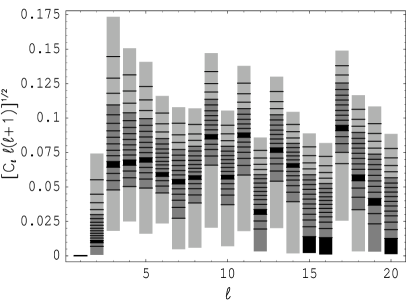
Figure 2: The COBE-DMR power spectrum. The vertical bands display the marginalized densities at each $\ell$. Horizontal bars mark off bins of constant probability. These bins are assigned their color in $C_{\ell}$ space and then projected into the diagram. The bin with the highest probability density is shown in black. The dark and light shaded regions are the 1-$\sigma$ and 2-$\sigma$ highest posterior density regions, respectively. The $C_{\ell}$ are measured in units $mK^{2}$ in this and all subsequent figures.

Figure 3: Marginalized posterior densities for each individual $C_{\ell}$ from the COBE-DMR data. At each $\ell$ the fluctuations in the $C_{\ell}$ at all other $\ell$ were integrated out. The axis ranges are the same for all panels.

IV Cosmic variance

In Eq. (9) we have written down the conditional posterior $P(C_{\ell}|s)$. This encodes what we know about the $C_{\ell}$ if we have perfect knowledge of the signal on the sky. The full posterior distribution $P(C_{\ell}|d)$ would reduce to this if we had perfect (noiseless, all-sky) data.

As shown in Eq. (9) the $C_{\ell}$ only depend on the data through $\sigma_{\ell}=\sum_{m=-\ell}^{+\ell}|s^{i}_{\ell m}|^{2}$. These $\sigma_{\ell}$ have a physical interpretation. They measure the actual fluctuation power on our sky. Therefore, if we had perfect data it would be possible to measure the $\sigma_{l}$ with zero variance.

The residual uncertainty in $C_{\ell}$ even for perfect data is a well known fact, known as cosmic variance. It is the consequence of having only one sky at our disposal, which means that there are a limited number of degrees of freedom for each $C_{\ell}$. Hence we cannot measure the $C_{\ell}$ arbitrarily precisely.

In this Bayesian treatment the functional form of the conditional posterior density may be unexpected. In the frequentist approach where the true underlying theory (i.e. the $C_{\ell}$) is thought of as fixed and the data as random, the variances on our sky $\sigma_{\ell}=\sum_{m}|s_{\ell m}|^{2}$ are thought of as $\chi^{2}$ variates with $2\ell+1$ degrees of freedom.

From a Bayesian perspective the data is fixed and our knowledge of the underlying theory is uncertain—so our knowledge about the $C_{\ell}$ is encoded in the inverse Gamma distributions $(2\ell-1)$, Eq. (9).

The mean and variance of the inverse Gamma distribution of order $d$ are

$$\langle C_{\ell}\rangle=\frac{\sigma_{\ell}}{d-2}\quad d>2,$$ (22)

and

$$\langle\Delta C_{\ell}^{2}\rangle=\frac{2\,\sigma_{\ell}^{2}}{\left(d-4\right)\,{\left(d-2\right)}^{2}}\quad d>4.$$ (23)

For the case of a flat prior $P(C_{\ell})=const$ we obtain $d=2\ell-1$. In this case the variance only becomes finite for $\ell>2$. This is a result of having chosen a flat prior for a variance measurement. There are in fact no arguments for doing so —when measuring a variance (which is a scale parameter) a flat prior does not correspond to maximal ignorance.

The Jeffrey ignorance prior for this case is $P(C_{\ell})=1/C_{\ell}$. This would lead to $d=2\ell+1$ and finite variance for $\ell>1$. In this case $\langle C_{\ell}\rangle=\frac{\sigma_{\ell}}{2\ell-1}$ and $\langle\Delta C_{\ell}^{2}\rangle=\frac{2\,\sigma_{\ell}^{2}}{\left(2\ell-3\right)\,{\left(2\ell-1\right)}^{2}}$.

In order to obtain the frequentist expectation $\langle C_{\ell}\rangle=\frac{\sigma_{\ell}}{2\ell+1}$ the prior $P(C_{\ell})=1/C_{\ell}^{2}$ would have to be used. In this case we still obtain a variance for the estimator which is larger by a factor $\frac{2\ell+1}{2\ell-1}$ than the frequentist chi-square variance knox1995 . So the mean of $P(C_{\ell}|d)$ is an unbiased estimator of $C_{\ell}$ for perfect data and hence has the same expectation as the maximum likelihood estimator Jewell .

These considerations are potentially relevant to the discussion about the statistical significance of the low $\ell$ $C_{\ell}$ estimates in the WMAP data in the Bayesian approach (e.g., EfstathiouQP and references therein). We will explore this issue in more detail in a future publication.

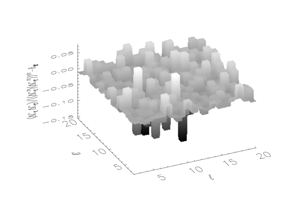
Figure 4: Correlation matrix of $C_{\ell}$ estimates from the COBE-DMR data. The diagonal components have been set to zero to enhance the contrast of the off-diagonal components. The surface is shaded according to height. We see that correlations between the power spectrum estimates vary between $8$% correlation at $(\ell,\ell^{\prime})=(6,10)$ and $15$% anti-correlation at $(\ell,\ell^{\prime})=(8,12)$. See Figure 5.

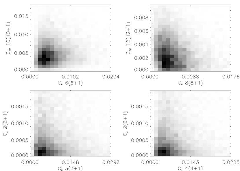
Figure 5: 2-D marginalized posterior densities. Each plot shows the full joint posterior of the data, integrated over all dimensions except for the two shown. From bottom left anti-clockwise: $P(C_{2},C_{3})$, $P(C_{2},C_{4})$, $P(C_{8},C_{12})$, and $P(C_{6},C_{10})$. The latter two were chosen because these $C_{\ell}$ pairs were maximally anti-correlated and correlated, respectively.

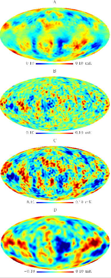
Figure 6: Reconstructed signal maps in Galactic coordinates. A: The signal component of the COBE-DMR data marginalized over the power spectrum: $\langle x\rangle|_{P(x|m)}$. This is a generalized Wiener filter which does not require knowing the signal covariance a priori. B: The solution $y$ of Eq. (11) at one Gibbs iteration. C: The sample pure signal sky $s=x+y$ at the same iteration (band-limited at $\ell_{max}=50$). D: The WMAP internal linear combination map smoothed to an FWHM of 5 degrees. The corresponding features in parts A and D are clearly visible. Note that in this map low galactic latitudes are not masked, which leads to some artifacts that are not visible in the masked COBE-DMR data.

V Computational Considerations

The computationally most demanding part of implementing this method is solving Eq. (10) and Eq. (11) at each iteration of the Gibbs sampler. Each of these is a linear system of equations of the form $Mv=w$, where $M=(1+S^{\frac{1}{2}}N^{-1}S^{\frac{1}{2}})$. It should be noted that these systems are of the same size as the map-making equation, Eq. (2). Maps also have to be made for approximate estimators. Therefore we expect the computational complexity of the Gibbs sampler to be no worse than the computational complexity of an approximate method.

For large $n_{p}$ $(n_{p}>10^{5})$ on the largest supercomputers available at the time of writing), direct solution of either of these equations becomes infeasible, because neither of them are sparse. This means the operation count scales as $n_{p}^{3}$ and because the memory requirements for storing the coefficient matrices scales as $n_{p}^{2}$. Therefore large systems of this type are usually solved using iterative techniques, such as the conjugate gradient (CG) technique numrec . The memory savings can be very large: the components of $M$ do not have to be stored as long as matrix vector products $Mv$ can be computed somehow. In terms of CPU time, iterative techniques outperform direct techniques if either $Mv$ can be computed in less than $n_{p}^{2}$ operations or the number of iterations required to converge to a solution of sufficient accuracy is much less than $n_{p}$.

We chose to write Eq. (10) and Eq. (11) in a form which satisfies all of theses requirements. The memory required is of order $n_{p}$ since we never need to store the components of the coefficient matrix.

The action of any power of $S$ on a vector can be computed in much less than $n_{p}^{2}$ operations using spherical harmonic transforms (or FFTs in the flat sky approximation). The action of $N^{-1}=A^{T}N^{-1}_{tod}A$ on a vector is generally easier to compute than the action of $N$ on a vector. As long as noise correlations can be modeled in a simple way in the time-domain (e.g. as piecewise stationary) the time required for applying $N^{-1}$ to a vector is similar to that required for a forward simulation of the data.

The number of CG iterations until convergence can be reduced far below the theoretical maximum $n_{p}$ if $M$ is nearly proportional to the unit matrix. This goal can be approached by finding an approximate inverse for $M$, a preconditioner.

If $N^{-1}$ were diagonal in the spherical harmonic basis, $M$ would be, too. Therefore, as long as this is approximately true on scales where $S\gg N$, a good preconditioner for this system would be the inverse of the diagonal part of $M$ in the spherical harmonic basis. These are easy to compute if we approximate the diagonal components of $N^{-1}$ by counting the number of $TOD$ samples in each pixel and weighting by the current noise temperature of the detector. Due to the way Eq. (10) and Eq. (11) have been written, the structure of $N^{-1}$ in the noise dominated regime does not matter, since if $S\ll N$, $M\approx 1$.

This preconditioner can be computed in $O(n_{p}^{\frac{3}{2}})$ operations. Figure 1 shows the results of a timing study for simulated data sets of varying size with WMAP-like scanning strategy and uncorrelated noise. The preconditioner performs well. The number of iterations does not increase with problem size over three orders of magnitude in $n_{p}$ and the computing time is is dominated by the spherical harmonic transforms.

VI Application to the COBE data

In order to test our method we applied to the well-studied COBE-DMR data. The exact maximum likelihood estimator gorskidmr ; gorskimoriond ; BJK and the least square quadratic estimator Tegmark have been computed for this data set. However, even for this small data set, the marginalized probability densities of each individual $C_{\ell}$, or the joint posterior density of pairs of $C_{\ell}$ have not been computed because doing so would require numerical integration over $\sim 20$ dimensions. We will show these densities here for the first time.

The COBE-DMR data COBE is published in the quadcube data structure, at a resolution which has 6144 pixels on the sphere. We use a noise-weighted average of the 53GHz and 90GHz maps. Because much of our code was already written for a HealPix data structure, we put the COBE data into a HealPix pixelization at resolution $n_{side}=64$ with $49152$ pixels. HealPix pixels whose centers lie within the same quadcube pixel get the same data (temperature) value.

Because the noise is completely correlated between sets of HealPix pixels in the same quadcube pixel, the noise covariance matrix $N$ is block diagonal, where each element of the block is $\sigma^{2}$, the published (noise) variance of that quadcube pixel. This means that $N$ is not strictly invertible, so we have to use a pseudo-inverse for $N^{-1}$. Our pseudo-inverse is also block diagonal, with constant-valued blocks, and correctly inverts the action of $N$ on a vector that is constant valued on the same blocks as $N$.

We project out the mean and dipoles from the uncut region of the COBE-DMR map, and model the data within the custom galactic cut as Gaussian random white noise with large variance. This corresponds to claiming complete ignorance of the foregrounds at low galactic latitudes (within the custom cut) and assuming that no residual foregrounds are present at high latitudes (outside the cut region). This is the simplest possible way of treating the monopole, dipole, and galactic foregrounds.

Our noise matrix has values published by the COBE team, but with the $\sigma^{2}$ noise variance increased to $1000\;mK^{2}$ in the galactic cut region, a numerically large value that exceeds any other variance in the problem.

For the first iteration of the Gibbs sampler we choose

$$C_{0}=C_{1}=10^{-30}\;\mbox{mK}^{2}\hskip 28.45274ptC_{\ell}=\frac{10^{-4}}{\ell(\ell+1)}\;\mbox{mK}^{2}.$$ (24)

We chose these values because they very roughly approximate the true $C_{\ell}$ values to reduce burn-in time. The first two are numerically small, because we consider the monopole and dipole to be non-cosmological. During the $C_{\ell}$ estimation step of the Gibbs sampler, the $C_{0}$ and $C_{1}$ values are not changed. This corresponds to enforcing the prior that the cosmological signal does not contain such components.

The Gibbs sampler is run through $10,000$ iterations (sets of $C_{\ell}$ values). This takes approximately 24 hours on an Athlon XP1800+ workstation. We ignore the first $1000$ iterations to ensure that the Gibbs sampler has converged to the true distribution. This is very conservative—in fact by computing correlations of our $C_{\ell}$ draws along the chain we infer that about every 20^th sample is uncorrelated.

We plot the power spectrum in figure 2. For each $\ell$ value, we display vertically a binned representation of the marginalized posterior densities $P(C_{\ell}|m)$. The bins all hold an equal number of points. The bins that are thinnest (points are densest in $C_{\ell}$ space) are colored more darkly. The top 68% are dark gray; from 68% to 95% are lighter gray, and the rest are white. The highest density bin is shown in black.

To explore the marginalized posterior $C_{\ell}$ distribution in more detail we plot their histograms in Figure 3. It is noteworthy that not a single one of these is even nearly Gaussian. Within the context of the discussion of the lack of large scale power in the CMB, it is worth pointing out that all inferences about $C_{2}$ from COBE-DMR can be based on the $P(C_{2}|d)$ shown here.

The correlation structure of the estimates contains information about how well we were able to account for the effects of the galactic cut. It is clear from figure 4 that the residual correlations are at most of order $10\%$ even at very small $\ell$.

However, since the posterior densities are non-Gaussian, the two-point correlations do not contain all the information. We therefore show the marginalized posteriors for four pairs of $C_{\ell}$s in figure 5. Again, all four of these densities are strongly non-Gaussian.

Lastly, we show the reconstructed signals. Figure 6A shows the expectation of the signal component (the solution of Eq. (10) at each iteration of the Gibbs sampler) of the COBE-DMR data with respect to the posterior density marginalized over the power spectrum: $\langle x\rangle|_{P(x|m)}$. This is a generalized Wiener filter (GWF) which does not require knowing the signal covariance a priori. The smoothing of the map autmatically adapts locally depending on how much detail the data support. The more strongly smoothed central horizontal band was obscured by the galaxy. Still the GWF reconstructs large scale modes in the galactic cut.

The power spectrum of figure 6A would be biased low, since the Wiener filter removes everything that could be noise. At each iteration of the Gibbs sampler the solution to Eq. (11) (shown in figure 6B) adds in a fluctuating term that replaces filtered noise with synthetic signal. It is noticable that this fill-in signal is larger in the regions of the map where the Galaxy obscures the CMB. The resulting draw $s$ from Eq. (6) is shown in figure 6C. Every $s$ draw is one possible pure signal sky that could have given rise to the data. Since we know that the COBE data has no statistical power above an $\ell_{max}$ of about 20, we imposed a bandlimit of $\ell_{max}=50$.

For comparison with the inferences we draw from the COBE-DMR data, we show in figure 6D the internal linear combination map from the WMAP satellite mapresults smoothed down to five degrees FWHM, an intermediate scale between the slightly larger average smoothing of panel A and the somewhat smaller smoothing of panel B and C due to the bandlimit of $\ell_{max}=50$. Nearly every hot and cold spot that is identified by the GWF can be found in the high signal-to-noise WMAP data. Figure 6C fills in signal very plausibly up to the imposed bandlimit. Even more striking is the similarity of our figure 6A to the combination of Q and V band WMAP data shown in figure 8 of mapresults , which is intended to mimic the COBE-DMR 53GHz map.

VII Conclusions and Future Work

We have described a framework for global and lossless analysis of cosmic microwave background data. This framework is based on a Bayesian analysis of CMB data. It has several advantages compared to traditional methods. It is computationally feasible. It is optimal and exact under the assumption of Gaussian fields and the ability to encode our prior knowledge about foreground components in terms of multivariate Gaussian densities. It uses controlled approximations (e.g. the number of samples of the Gibbs sampler controls the accuracy of the result but this can be increased by spending more computing time). It allows joint analysis of the CMB signal, foregrounds and noise properties of the instrument, while modeling and exploiting the statistical dependence between these different inferences.

Traditional methods of inference from CMB data divide the data analysis into several steps: map-making from TOD, component separation, power spectrum estimation from the CMB signal and cosmological parameter estimation. Our method allows treating all these inferences jointly and self-consistently, if desired. The traditional results can be understood as special cases of our method for certain uninformative prior choices. For example, pure map-making could be viewed as applying this framework with $P(s|C_{l})P(f)P(C_{l})=const$.

In spite of this generality, the framework for analyzing CMB data described here is very modular: the structure of the Gibbs sampling scheme separates the different steps of the inference process focusing on each component in turn. The framework described here therefore holds the promise of making more data analysis steps part of a self-consistent framework rather than sequential stages in a data pipeline.

Our method turns out to give an unbiased Wiener filter and generalizes the global filtering and reconstruction methods in rybickipress to include power spectrum estimation, obviating the need for a priori knowledge of the signal covariance.

We require the use of iterative techniques to solve the most computationally demanding step in this method. We find that our simple-minded preconditioned gradient iteration works well over 3 orders of magnitude in problem size. It remains to be studied whether other preconditioners may be even more effective (e.g. pen ).

We applied our formalism to the well-studied COBE-DMR data set. We demonstrate that our methods enable new analyses for even such a small data set. We quote posterior densities for individual $C_{\ell}$ as well as posterior densities for pairs of $C_{\ell}$ as examples of results that would be prohibitively expensive to obtain with traditional algorithms. Our results are consistent with the most sophisticated brute force $O(n_{p}^{3})$ analyses available in the literature.

The approach can be extended straightforwardly to polarized maps, data that spans different frequency bands and joint estimation of different data sets. There is nothing that prevents the application of these ideas to random fields on manifolds other than the sphere, such as one-, two- or three-dimensional Euclidean space. We are investigating the formalism for joint inference from CMB data about the power spectrum and map of the pure CMB sky with the power spectrum and map of the projected gravitational potential. We will report on these developments in a future publication.

Appendix A Analytic Marginalization Over Foregrounds

From a statistical point of view we consider the a posteriori distribution to be a function of the CMB signal, $C_{\ell}$ and the foregrounds. Then we marginalize over the foregrounds $f$. This can be done either implicitly through Gibbs sampling from the joint posterior density including $f$ (as described in the main text) and then marginalizing over $f$ in the generated samples or explicitly through analytic marginalization of the posterior over $f$. Then the ignorance about the foreground is included in additional terms in the noise covariance matrix. The first route is more general, but there may be occasions where the second is preferable; for example if the main goal is to make the CMB analysis insensitive to a small number of known foreground templates $f_{i}$.

The effect of analytic marginalization is that the new noise covariance matrix $N^{\prime}$ including the foreground term becomes

$$N^{\prime}\equiv N+\sigma_{f}^{2}FF^{T}\equiv N+\sigma_{f}^{2}\sum_{i}f_{i}f_{i}^{T}.$$ (25)

In order to implement the Gibbs sampler including this new term we need to be able to apply ${N^{\prime}}^{-1}$ to vectors. If only a small number (up to $\sim 1,000$) of foreground templates need to be projected out this can best be done by grouping all the vectors using the following limit of the Sherman-Morrison-Woodbury formula rybickipress

$$N^{\prime-1}\equiv\lim_{\sigma_{f}^{2}\rightarrow\infty}(N + \sigma_{f}^{2}FF^{T})^{-1}=$$ (26)

$$N^{-1} - \left[N^{-1}F\left(F^{T}N^{-1}F)^{-1}F^{T}N^{-1}\right)\right].$$

This operation will project out the directions in $N^{-1}$ corresponding to the foreground contributions. The action of this new inverse noise covariance matrix on a vector can be computed using methods similar to those described in Eqs. (2.7.16ff) in numrec .

Alternatively one can solve iteratively the set of equations

$$\left(N+\sigma_{f}^{2}FF^{T}\right)x=v$$ (27)

every time $x=N^{\prime-1}v$ is required on the LHS of Eq. (10) and Eq. (11). When $N^{\prime-\frac{1}{2}}$ is required for the RHS of Eq. (11) we solve

$$\left(N+\sigma_{f}^{2}FF^{T}\right)y=N^{\frac{1}{2}}\xi+\sigma_{f}F\chi.$$ (28)

The term $N^{\frac{1}{2}}\xi$ is obtained by simulating a noise-only map solving Eq. (2) with $d=n_{tod}$. In both of these equations one can choose $\sigma_{f}$ numerically large.

However, the method in the main text is more flexible, since it allows grouping different foregrounds together in ways that are computationally convenient.

References

- (1) W. Hu and S. Dodelson, Ann. Rev. Astron. Astrophys. 40, 171 (2002)
- (2) A. D. Milleret al. 1999 Astrophys.J. 524 (1999) L1-L4; N. W. Halverson et al. 2001, astro-ph/0104489; S. Hanany et al. Ap. J. 545 (2000) L5; K. Grainge et al. Mon. Not. R. Astron. Soc. 000, 1 5 (2002); Kuo, C. L. et al. 2002, Ap. J., astro-ph/0212289; J. E. Ruhl et al. (2002), astro-ph/0212229; S., Padin et. al., Ap. J. 549, L1, (2001)
- (3) C. L. Bennett et al., astro-ph/0302208, Ap. J., in press.
- (4) J. R. Bond and G. Efstathiou, MNRAS 226, 655 (1987)
- (5) M. Tegmark, Phys. Rev. D55, 5895 (1997)
- (6) J. R. Bond, A. H. Jaffe, and L. Knox, Physical Review D 57, 2117 (1998)
- (7) K. M. Górski, E. Hivon, B. D. Wandelt, Evolution of large scale structure : from recombination to Garching /edited by A. J. Banday, R. K. Sheth, L. N. da Costa. Garching, Germany : European Southern Observatory, 37 (1999)
- (8) J. R. Bond, R. Crittenden, A. Jaffe, L. Knox, Comput.Sci.Eng.1, 21 (1999)
- (9) J. Borrill, Phys.Rev.D 59, 027302 (1999)
- (10) S. P. Oh, D. N. Spergel, G. Hinshaw, Ap. J. 510, 551 (1999)
- (11) B. D. Wandelt, F. Hansen, astro-ph/0106515, Phys. Rev. D 67, 023001 (2003)
- (12) B. D. Wandelt, E. Hivon, and K. M. Górski, Phys. Rev. D 64, 083003 (2001)
- (13) E. Hivon et al., Ap. J. 567, 2 (2002)
- (14) Szapudi et al.,, Ap. J. 548, L115 (2001)
- (15) G. P. Efstathiou, astro-ph/0307515, submitted to MNRAS.
- (16) G. P. Efstathiou, astro-ph/0306431, submitted to MNRAS.
- (17) J. Jewell, S. Levin, and C. H. Anderson, astro-ph-0209560, submitted to Astrophysical Journal.
- (18) J. R. Bond, A. H. Jaffe, and L. Knox, Astrophysical Journal 533, 19 (2000)
- (19) J. Bartlett et al, Astrophysical Letters and Communications, 37, 321 (2000)
- (20) L. Verde et al 2003, astro-ph/0302218, Ap. J., in press.
- (21) L. Knox, Phys. Rev. D 52, 4307 (1995)
- (22) K. M. Gorski, et al., Ap. J. 464, L11 (1996)
- (23) K.M. Górski, Cosmic Microwave Background Anisotropy in the COBE DMR 4-yr Sky Maps, Proceedings of the XXXIst Recontres de Moriond, ’Microwave Background Anisotropies’, astro-ph/9701191 (1998)
- (24) C. L. Bennett et al., Ap. J. 464, L1 (1996)
- (25) G. B. Rybicki and W. H. Press, Astrophysical Journal 398, 169 (1992)
- (26) Tanner, Tools for Statistical Inference: Methods for the Exploration of Posterior Distributions and Likelihood Functions, 3rd Edition. Springer Verlag, Heidelberg, Germany. (1996)
- (27) W. H. Press, et al., Numerical Recipes. Cambridge University Press, Cambridge, England. (1992)
- (28) U. L. Pen, astro-ph/0304513, MNRAS in press.