Arecibo 430 MHz Pulsar Polarimetry: Faraday Rotation Measures and Morphological Classifications

Abstract

We have measured Faraday Rotation Measures $(RM)$ at Arecibo Observatory for 36 pulsars, 17 of them new. We combine these and earlier measurements to study the galactic magnetic field and its possible temporal variations. Many $RM$ values have changed significantly on several–year timescales, but these variations probably do not reflect interstellar magnetic field changes. By studying the distribution of pulsar $RM$s near the plane in conjunction with the new NE2001 electron density model, we note the following structures in the first galactic longitude quadrant: (1) The local field reversal can be traced as a null in $RM$ in a 0.5–kpc wide strip interior to the Solar Circle, extending $\sim 7$ kpc around the Galaxy. (2) Steadily increasing $RM$s in a 1–kpc wide strip interior to the local field reversal, and also in the wedge bounded by $42<l<52\arcdeg$, indicate that the large–scale field is approximately steady from the local reversal in to the Sagittarius arm. (3) The $RM$s in the 1–kpc wide strip interior to the Sagittarius arm indicate another field reversal in this strip. (4) The $RM$s in a final 1–kpc wide interior strip, straddling the Scutum arm, also support a second field reversal interior to the Sun, between the Sagittarius and Scutum arms. (5) Exterior to the nearby reversal, $RM$s from $60<l<78\arcdeg$ show evidence for two reversals, on the near and far side of the Perseus arm. (6) In general, the maxima in the large–scale fields tend to lie along the spiral arms, while the field minima tend to be found between them.

We have also determined polarized profiles of 48 pulsars at 430 MHz. We present morphological pulse profile classifications (Rankin, 1983) of the pulsars, based on our new measurements and previously published data.

1 INTRODUCTION

We have determined full–polarization properties of 48 pulsars at 430 MHz from Arecibo Observatory. This paper presents the principal results of these measurements–Faraday rotation and interstellar magnetic field determinations, and polarized profiles and pulsar morphological classifications. The plan of the paper is as follows: In the remainder of the Introduction, we summarize the background on these two primary results. The second section of the paper describes the observations and our analyses of them. The third section discusses our Faraday rotation and galactic magnetic field results in detail, while the fourth describes the polarized profiles and morphological classifications. Conclusions are given in the fifth section.

1.1 Faraday Rotation and Interstellar Magnetic Field Measurements

Pulsars are ideal probes of the galactic magnetic field. Faraday Rotation measurements of pulsars’ linearly polarized emissions yield the Rotation Measure, $RM$, which is a path integral along the line of sight involving the magnetic field $B$ and electron density $n_{e}$:

$$RM=0.81\int\limits_{PSR}^{\earth}{n_{e}{\bf B}\cdot d{\bf s}};$$ (1)

while pulse timing measurements determine the Dispersion Measure, $DM$, which is another path integral along the line of sight involving electron density $n_{e}$ alone:

$$DM=\int\limits_{PSR}^{\earth}{n_{e}ds}.$$ (2)

Consequently the mean value of the component of the magnetic field along the line of sight, $<B_{||}>$, is given by:

$$\left\langle{B_{||}}\right\rangle=\int\limits_{PSR}^{\earth}{n_{e}{\bf B}\cdot d{\bf s}\;}/\int\limits_{PSR}^{\earth}{n_{e}ds\;}=RM/(0.81DM).$$ (3)

The galactic magnetic field structure is particularly amenable to study with pulsars because of this relationship, which can be evaluated with pulsars at various distances along a particular line of sight. Indrani & Deshpande (1998) and Han et al (1999) provide recent comprehensive analyses of the galactic magnetic field.

1.2 Pulsar Morphological Classifications

Rankin (1983) proposed a morphological pulsar classification scheme that was based on examination of multifrequency, polarized pulse profiles. Rankin found that there are two principal classes of emission beams – core and conal, whose properties are distinguishable through careful analysis of polarized properties as a function of frequency. She and others have applied her classification criteria to large number of pulsars in subsequent papers (Rankin 1986, 1990, 1993; Rankin, Stinebring, & Weisberg 1989; Weisberg et al 1999). In the current paper, we measure a large number of polarized profiles at 430 MHz, and use them and earlier multifrequency measurements to make new morphological classifications and to improve old ones.

2 OBSERVATIONS AND ANALYSIS

The data were gathered with the dual–circularly polarized 430 MHz linefeed at Arecibo Observatory. A 5 MHz band centered at 430 MHz was fed into the Arecibo correlator, and 32 lags of auto– and cross–correlation functions were formed every $400~{}\mu s$. Using an ephemeris for the apparent pulsar period generated by program TEMPO (Taylor & Weisberg, 1989) to calculate the pulsar rotational phase at the epoch of each such sample, we selected one of 1024 pulse longitude bins to accumulate the resulting four correlation functions. This procedure continued for 120 seconds of observing. Off–line, the four correlation functions at each longitude bin were three–level corrected and Fourier transformed to form pulse profiles in the four Stokes parameters. This procedure was essentially identical to that used in the 21 cm observations of Weisberg et al (1999), except that the 430 MHz linefeed limited the bandwidth to a narrower range. At this point in the processing, the data consisted of a cube of 1024 longitude bins x 4 Stokes parameters x 32 frequency channels of 156.25 kHz bandwidth, representing a two minute integration or “scan.”

2.1 Faraday Rotation Measurements

Observationally speaking, the Faraday Rotation Measure $RM$ is conventionally expressed as a rotation of the linearly polarized position angle $\psi$ as a function of wavelength $\lambda$:

$$\psi-\psi_{0}=RM\;\lambda^{2};$$ (4)

where $RM$ has units of rad m^-2. The rate of rotation with wavelength is then

$${d\psi\over d\lambda}=2\;RM\;\lambda$$ (5)

It is more convenient for us initially to measure it as a position angle rotation rate with frequency:

$${d\psi\over d\nu}=-{2\;RM\;c^{2}\;\over\;\nu^{3}}$$ (6)

At our center frequency of 430 MHz, then, the conversion between rotation rate $d\psi/d\nu$ and $RM$ is simply

$${d\psi\over d\nu}=-0.12953\;{RM\over{\rm rad\;m}^{-2}}\;{\rm deg\over MHz};$$ (7)

so we will use the two quantities interchangeably in what follows.

The linearly polarized position angle $\psi$ suffers a significant net rotation across the 32 frequency channels owing to interstellar and ionospheric Faraday rotation plus an instrumental position angle rotation term, respectively:

$${d\psi\over d\nu}|_{net}={d\psi\over d\nu}|_{ISM}+{d\psi\over d\nu}|_{Iono}+{d\psi\over d\nu}|_{Instr}.$$ (8)

In order to determine the interstellar component of the rotation and hence the interstellar magnetic field, and also to produce polarized pulse profiles not suffering significant linear depolarization, we next determined the net position angle rotation rate across the bandpass $d\psi/d\nu|_{net}$ and derotated the linear polarization at each frequency by this amount.

To measure this position angle rotation rate with frequency, we performed two successively finer grid searches at a given longitude bin, as follows (see Fig. 1). First we chose each of 260 trial $\psi$ derotation rates corresponding to $RM$s between $\pm 2000$ rad m^-2, and then summed the derotated linear Stokes parameters $Q$ and $U$ across the 32 frequency channels. Our first estimate of net derotation rate of position angle with frequency was the one that maximized $L$ in this first trial process. Then we recentered the search on this first estimate; and did 11 trial $\psi$ derotation rates corresponding to $RM$s within $\pm 15$ rad m^-2 of this value. We then fitted a parabola to the peak of the latter curve. The adopted derotation rate of position angle with frequency, $-d\psi/d\nu|_{net}$, was the one that maximized $L$ in this process. The procedure was repeated at every longitude bin for which there was significant linearly polarized power (typically $L\geq 3\sigma_{L}$), and a weighted average derotation for the two–minute scan, $<-d\psi/d\nu>|_{net}$, was then computed from the results at each longitude (see Fig. 2). The uncertainty was taken to be the standard deviation of the mean.

To extract the interstellar Faraday rotation from the measured $<d\psi/d\nu>|_{net}$, it is necessary to subtract the ionospheric and instrumental contributions (cf. Eqn. 8). To estimate the ionospheric Rotation Measure, we integrated a time–dependent model of the ionospheric electron density [International Reference Ionosphere 1995; (Bilitza , 1997)] and geomagnetic field [International Geomagnetic Reference Field 1995; (Barton , 1997)] through the ionosphere along the Arecibo–pulsar line of sight, yielding typical $RM|_{Iono}\sim(0.5-4)$ rad m^-2.

The instrumental rotation rate across the bandpass was assumed to be constant during each given daily session, and was taken as the weighted difference between our measured Rotation Measures and the published values for six “$RM$ calibrator pulsars.” (The uncertainty in this quantity is the standard deviation of the mean difference.) Consequently our values depend on the correctness of previously published results and their constancy over time. Our calibrator list initially included every one of our pulsars that additionally had a published $RM$ value. It quickly became clear that most of the published values were not correct at our observing epoch, as they did not yield an instumental rotation consistent with other pulsars. We finally arrived at our final list of only six “$RM$ calibrator pulsars” (see Table 1) whose published $RM$’s could be reconciled with our observations.

After determining the ionospheric and instrumental rotation rates as described above, we derived interstellar Rotation Measures for each 2–minute scan for all of our pulsars via Eqn. 8. Our final measured interstellar $RM$ for each pulsar was the weighted average of these results.

Comparison of our resulting “measured” interstellar $RM$’s with the published values for the Calibrator pulsars constitutes a closed-loop test of our calibration system, as we processed these pulsars identically as the others we observed. Note that our “measured” values indeed agree with the published values for these pulsars to within the errors. (See Table 1.) The many other pulsars’ published $RM$’s that disagree with our measurements will be discussed below.

2.2 Final Polarized Pulse Profiles

The weighted average position angle derotation $<-d\psi/d\nu>|_{net}$ was applied to the Stokes parameter profiles at each of the 32 contiguous frequencies, and they were then summed to form a polarized profile for the scan. Each scan on a given pulsar was crosscorrelated in two dimensions with a high $S/N$ full–Stokes profile template, in order to shift it in time and position angle before accumulating it into a “grand average.” Specifically, we first cross–correlated the total power $(I)$ scan and template as a function of longitude to obtain the time offset of each scan with respect to the template, and we rotated the scan’s polarized profile in time by this amount. Next, we crosscorrelated the linearly polarized $Q+iU$ scan and template profiles as a function of position angle offset to determine the best offset in $\psi$ between them, and we then rotated the scan’s linearly polarized position angle by this amount. Finally, the time– and position angle–registered profile was accumulated into a grand average waveform, as shown in Figs. 10–22. We use the IEEE convention for defining circular polarization (Kraus, 1966), in which left circularly polarized radiation is defined as that which is transmitted and received by a left-handed helix. The Stokes parameter $V=S_{\rm left}-S_{\rm right}$.

We estimate that in the worst cases, $V$ could be systematically in error by $\pm 5\%$ of $I$ due to the difficulty in calibrating left– versus right– circularly polarized radiometer channels via standard source observations in crowded fields. Additional possible errors in $V$ of up to $\pm 0.15L$ due to instrumental polarization were averaged down in most cases by multiple observations.

These data were gathered in seven daily observing sessions from 1991 December through 1992 December. The profile resolution is $1/1024$ of the pulse period, or $0\fdg 3516$. For the weaker pulsars, the profile is boxcar–smoothed. If such smoothing was done, the number of channels in the boxcar is listed in the figure caption.

For those pulsars exhibiting little or no linear polarization, it is possible that an incorrectly determined rotation measure has depolarized any intrinsic linear polarization. However, our rotation measure finding algorithm should have found the correct $RM$ if indeed there was sufficient $S/N$ in $L$.

3 ROTATION MEASURES AND INTERSTELLAR MAGNETIC FIELDS

In the following sections, we present our new $RM$ measurements. We then study both time variations in $RM$, and the large–scale structure of galactic magnetic fields.

3.1 Measured RMs and Time Variations

Table 2 lists our rotation measures, previously published values (where available), and the difference between them. Note that many of our determinations differ from earlier measurements by more than the joint uncertainties, suggesting that time variations are common. van Ommen et al (1997) and Han et al (1999) also list several pulsars having $RM$s varying by several rad m^-2 on timescales of years.

Eq. 3 shows that $RM$ variations might result either from magnetic field or electron density variations (or both). It is possible to test for the level of electron density variations if multiepoch dispersion measure ($DM$) values are available. While some pulsar $DM$s show very small time variations (Phillips & Wolszczan 1991; Backer et al 1993), others vary by several percent on these timescales (D’Alessandro et al., 1993). van Ommen et al (1997) found that $RM$s and $DM$s tended to vary in a correlated fashion, while Manchester (1974) detected a change in the $RM$ of PSR B0329+54 without accompanying $DM$ variations.

Fortunately, we are able to investigate possible sources for the $RM$ changes in our pulsars because Hankins & Rankin (2003) measured $DM$s of many of them at approximately the same epoch as we gathered our $RM$ data. Table 3 displays their and earlier $DM$ measurements on many of our $RM$ pulsars. It is clear from comparison of the percentage changes in Tables 2 and 3 that $RM$s tend to vary far more on a several–year timescale than do $DM$s. Consequently it is evident that electron density variations are not responsible for the bulk of the $RM$ changes.

Of course pulsars embedded in supernova remnants such as Vela and the Crab Nebula, show large variations of both $RM$ and $DM$ (Hamilton et al 1985; Rankin et al 1988). The largest difference in Table 2 between previously published and our measured $RM$s is for PSR J1532+2745=B1530+27, which does not lie in an SNR. We have no other explanation for the discrepancy. Multiple observations at several of our observing epochs confirm our $RM$ result on this pulsar.

While it appears from the above arguments that the temporal changes in $RM$ must result from interstellar magnetic field variations, caution is required. Recent work by Ramachandran et al. (2003) shows that large variations in $RM$ as a function of pulse phase are seen in some pulsars. (Our error analysis procedure accounts for these variations, so that our tabulated values and uncertainties in $RM$s reflect this phenomenon.) Ramachandran et al. (2003) also demonstrate that this (spurious) apparent $RM$ variation with pulse phase can result from average–pulse measurements of a pulsar having a quasi–orthogonal polarization mode emission process. Time variations in apparent $RM$ could then result from the balance of the two modes shifting slightly over time, rather than from interstellar magnetic field changes.

3.2 The Galactic Magnetic Field in Selected Directions

In the following sections, we use our new pulsar $RM$ data in conjunction with previously measured values [summarized in Manchester (2002) and supplemented by recent measurements of Mitra et al (2003)] to probe the galactic magnetic field structure in selected directions. Global analyses can be found in Han et al (1999) and Indrani & Deshpande (1998). While the random component of the field is comparable to or even larger than the systematic structure (Ohno & Shibata, 1993); we focus here on the systematic part. In order to investigate the field as a function of location in the Galaxy, we use the NE2001 electron density model (Cordes & Lazio, 2002) and the pulsar dispersion measure $DM$ to determine the distance to each pulsar studied. In most cases, we select wedges of longitude along the galactic plane for our studies, setting the longitude boundaries to isolate global magnetic field structures. (In all cases we have limited our studies to those pulsars with galactic latitudes $|b|<9\arcdeg$). In one case where a wedge cannot segregate the desired magnetic structure, we instead select a region lying within a given distance range of a particular spiral arm. While the NE2001 model yields distances with typical uncertainties of some tens of percent, the relative distances of various pulsars should be roughly correct within sufficiently small zones. Since the rotation measure $RM$ is a path integral of the magnetic field, a steady large–scale field will tend to appear as a constant slope (modulo changes in $n_{e}$) in plots of $RM$ versus distance, and a magnetic field reversal will lead to a change in the sign of the slope. Note also from Eq. (1) that a positive (negative) $RM$ indicates that the radio signal is propagating parallel (antiparallel) to the field.

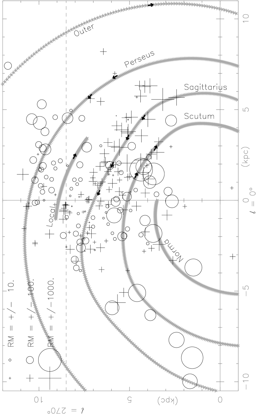
Figure 3: $RM$s of low–latitude pulsars in the Galaxy, from Manchester (2002), Mitra et al (2003), and this work. The horizontal dashed line intersects the y–axis at the Sun, at coordinates $(0.0,8.5)$ kpc. The arrows indicate schematically the direction of the field as ascertained from this work (see Figs. 4 – 9 and text for further discussion). The spiral arms are generated from routines provided by Cordes & Lazio (2002).

To set the overall context while invesigating particular zones, the reader may examine a map of the galactic plane plotting all known low–latitude pulsar $RM$s (see Fig. 3), with superposed global field directions deduced from this work. This figure also displays the spiral arms as presented by Cordes & Lazio (2002).

3.2.1 Field Reversal Just Inside the Solar Circle

It is difficult to analyze a magnetic field reversal when the reversal lies along a line oriented close to, but not parallel to, the line of sight. Looking at pulsar $RM$s within a longitude wedge in this situation can be misleading because the reversal does not lie at a unique longitude. Pulsars at similar longitudes and distances from the Sun, but on opposite sides of a reversal, may have drastically different $RM$s. Consequently in this situation we use different selection criteria than longitude. It is useful to select pulsars within some given distance range from the nearest spiral arm in order to examine whether the magnetic field reversal follows the galactic spiral pattern. With suitable adjustment of this distance window, we can see magnetic field effects for a very narrow and precise region of the interstellar medium near the spiral arms. For example we can investigate whether a reversal does indeed lie at a constant distance from a spiral arm.

The rotation measure depends upon four quantities, as seen from Eq. (1) – distance, $n_{e},B$, and the angle between the propagation vector and the magnetic field. Hence it is important to note that plots of $RM$ against distance cannot by themselves discriminate among the several factors that may affect $RM$. This conclusion holds whether one selects pulsars within either a wedge or a strip of the Galaxy.

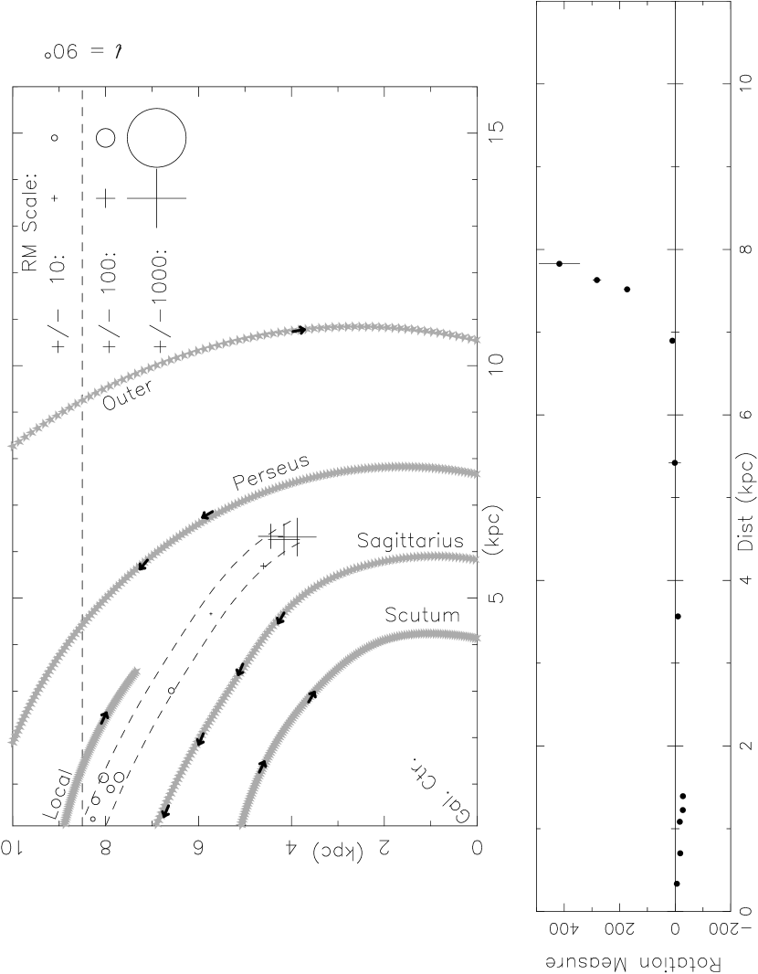
Figure 4: $RM$s of pulsars lying from 1.0 to 1.5 kpc outside the Sagittarius arm (the first arm inside the Solar Circle), roughly in the $l\sim 60\arcdeg$ direction and near the galactic plane $(|b|<9\arcdeg)$. Top: The selected region is delineated by curving dashed lines. See Fig. 3 caption for additional details. Bottom: $RM$ versus distance in the selected region. Note that there is a clear null in the magnetic field all the way from the solar vicinity out to $d\sim 7$ kpc.

The field reversal thought to exist several hundred pc inside the Solar Circle (Thomson & Nelson 1980; Han & Qiao 1994; Rand & Lyne 1994) is such a case. The field is clockwise near the Sun when viewed from above; inside the reversal it changes to counterclockwise from above (see Fig. 3). Rand & Lyne (1994) found negligible $RM$s throughout the wedge $60<l<80\arcdeg$ for all pulsars within about 5 kpc of the Sun, and attributed the null to a large–scale field reversal. Their result is no longer supportable with the larger number of measurements accumulated since then. In fact we find that there is no unique longitude range in this vicinity that traces the null for great distances. However, for the strip lying approximately midway between the Local arm and the Sagittarius (next inner) arm toward $l\sim 60\arcdeg$– specifically from (1.0–1.5) kpc outside the Sagittarius arm (see Fig. 4), we find that $RM$s cluster near zero for the first 7 kpc from the Sun. Because these pulsars are at varying distances from the Sun (from 0.3 to nearly 7 kpc), we must be looking along an actual null in the magnetic field extending for $\sim 7$ kpc. In this case, instead of surmising the existence of a reversal on the basis of trends in the sign of $RM$, we clearly see the reversal itself. We also find that if we widen the zone much beyond our current limits, the $RM$s tend systematically away from zero as expected on opposite sides of a reversal. (See below for details.) Therefore it appears that the null is confined to a width of less than 0.5 kpc over the 7 kpc range. It is important to emphasize that this null, whose location is now by far the best–known for any large–scale field reversal in the Galaxy, clearly lies midway between arms rather than along one.

The rapid, systematic rise in $RM$ for $d>7$ kpc signals that the null no longer lies $\sim 1$ kpc outside the Sagittarius arm here. Unfortunately, there are not enough pulsars with measured $RM$s near and beyond here to map out exactly what is happening in this vicinity, but we note that the Local arm is presumed to end and the Perseus (next outer) arm also approaches closer to the Sagittarius arm near here. Presumably these global galactic structures are perturbing the well–behaved pattern that we were able to trace out for a considerable distance up to this location. $RM$ measurements of additional, more distant pulsars in this direction will help to clarify the situation.

We have also investigated the local reversal in the opposite direction, i.e., toward $l\sim 270\arcdeg$. The reversal is not nearly as well–defined, but in general the trend is consistent with what is found toward $l\sim 60\arcdeg$ (see Fig. 3): The local field reversal midway between the Local arm and the next arm interior to it (Sagittarius) separates clockwise fields near the Local arm from counterclockwise fields near the next interior one; causing predominantly positive $RM$s in the former case and negative ones in the latter. The few counterexamples probably result from Faraday screens along particular lines of sight, a point emphasized by Mitra et al (2003). The overall field structure at large distances toward $l\sim 280\arcdeg$ is unknown because of perturbations caused by the Gum Nebula.

3.2.2 Field Structure Interior to the Nearby Field Reversal

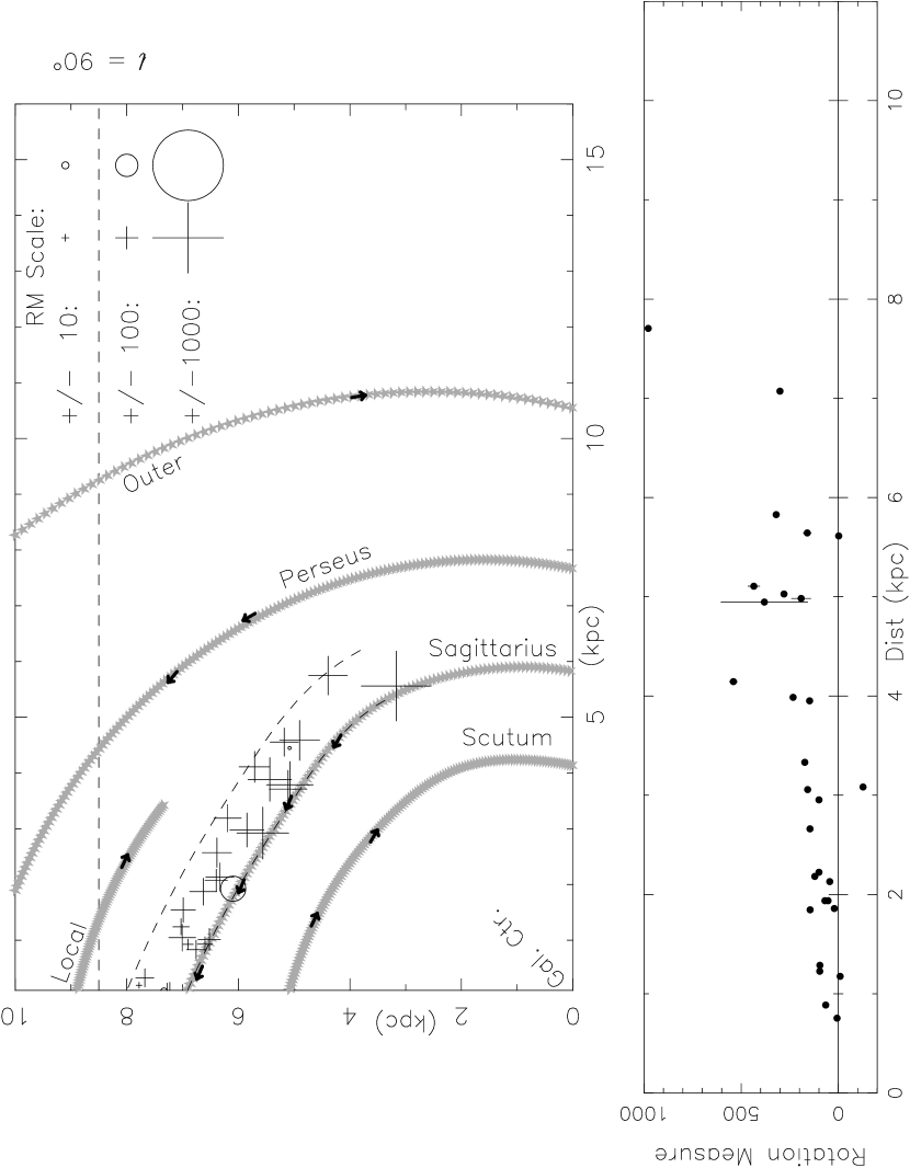
Figure 5: $RM$s of pulsars lying in the region between the Sagittarious arm and 1.0 kpc exterior to it near the galactic plane $(|b|<9\arcdeg)$. Top: The selected region is delineated by curving dashed lines. See Fig. 3 caption for additional details. Bottom: $RM$ versus distance in the selected region. Note that a constant magnetic field would lead to a constant slope (modulo variations in $n_{e}$) in this plot, since $RM$ is a path integral quantity.

We next investigate the field lying in three 1–kpc wide strips interior to the nearby field reversal. The first segment selects pulsars from the reversal inward to the Sagittarius arm. (See Fig. 5.) Note the clear trend of increasing $RM$ with distance, which indicates that the field is relatively steady in this region. The narrow wedge from $42\arcdeg<l<52\arcdeg$, whose inner edge cuts just inside the Sagittarius arm (see Fig. 6), also illustrates that the field from the local reversal in to Sagittarius arm is approximately steady, as there is again a regular trend of increasing $RM$ with distance. Most extragalactic sources in this direction exhibit $RM\sim 500$ rad m^-2 (Clegg et al, 1992), so there is no evidence for additional major reversals beyond the pulsars.

The second strip interior to the local field reversal selects pulsars from the Sagittarius arm to 1 kpc on its interior side. (See Fig. 7.) The general trend of $RM$ with distance in this strip is similar to that in the first region. As $RM$ is a path integral quantity, this similarity suggests that a second low–field region (i.e., a second reversal) is being traversed somewhat interior to the Sagittarius arm. The farther pulsars in these two strips tend to show higher $RM$s because their signals propagate more nearly parallel to the field.

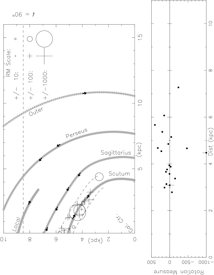
Figure 8: $RM$s of pulsars lying in the region between 1 and 2 kpc interior to the Sagittarious arm, roughly atop the Scutum arm, near the galactic plane $(|b|<9\arcdeg)$. Top: The selected region is delineated by curving dashed lines. See Fig. 3 caption for additional details. Bottom: $RM$ versus distance in the selected region.

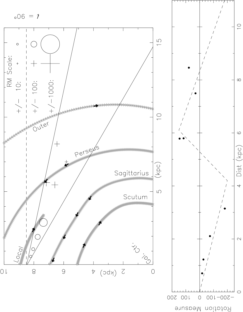
Figure 9: $RM$s of pulsars lying in the range $60<l<78\arcdeg$ near the galactic plane $(|b|<9\arcdeg)$. Top: The selected region is delineated by a wedge. See Fig. 3 caption for additional details. Bottom: $RM$ versus distance in the selected region. Extragalactic Source $RM$s in this direction are negative (Clegg et al, 1992). The dashed line illustrates schematically the trends in $RM$ versus $d$, suggesting field reversals before and after the Perseus arm. (Note that a field reversal leads to a change in the sign of the slope of $RM$ versus distance, since $RM$ is a path integral quantity.)

The third strip interior to the local reversal, (see Fig. 8), which encompasses the Scutum arm, shows more negative $RM$s than the first and second strips, especially at larger distances. This indicates that these pulsars’ signals begin their journey through a sufficiently long region of clockwise field near the pulsar, before reaching the second reversal described above, to approximately nullify the opposite field along much of the rest of the path. (See the arrows on Fig. 9, which sketch the deduced field directions).

It is interesting to note that our work suggests that both of the nulls/reversals lie between arms, while Indrani & Deshpande (1998), Han et al (1999), and Han et al (2002) indicate maximal field magnitude in these regions. Much of the discrepancy can be attributed to the new NE2001 electron density model bringing most pulsars closer to Earth, while some of the change is due to adjustments in the location of the spiral arms themselves. [Han et al (2002) find yet another (third) reversal even farther in, also near an arm – the Norma arm. The latter $RM$s have not yet been published so we are not able to study them with the aid of the new NE2001 model – determined distances.]

3.2.3 Field Reversals External to the Solar Circle

We next investigate the longitude range $l\sim(60-78)\arcdeg$ [see Fig. 9]. The lower longitude limit of this wedge ensures that lines of sight remain exterior to the local reversal which lies just inside to the Solar Circle. The nearest several kpc of the wedge skim near or along the Local arm. The $RM$s near the Sun grow more negative with distance out to $d\sim 3$ kpc, as expected from a clockwise local magnetic field. Yet in the range 6 $\lesssim$ $d$ $\lesssim$ 8 kpc, $RM$s are positive; while extragalactic $RM$s are again negative (Clegg et al, 1992). Consequently two field reversals, each corresponding to a change of slope in $RM$ versus distance, are required at $d\sim 4.5\pm 1$ kpc and $d\gtrsim 6$ kpc, as indicated schematically on the Figure. The nearer reversal is located interior to the Perseus (next outer) arm; the farther reversal somewhere beyond it. As in the interior Galaxy, we find that reversals/nulls tend to occur between arms. (The field between these two exterior reversals, near the Perseus arm, is counterclockwise [see Fig. 3].) Han et al (1999)also suggested that there may be two reversals exterior to the Sun; our contribution rests in providing several new measurements and in the application of the NE2001 model to estimate distances, both of which refine the arguments for two exterior reversals, at least in this direction. Note however that there is no clear evidence for reversals toward or beyond the Perseus arm at higher longitudes (Brown & Taylor 2001; Mitra et al 2002).

4 POLARIZED PROFILES AND MORPHOLOGICAL CLASSIFICATIONS

Figures 10 – 22 show the full polarization profile for each pulsar. (In a few instances, linear $(L)$ and/or circular $(V)$ polarization is not displayed because it is too weak.) We discuss each profile and its classification below. The classifications are based on the Rankin (1983) morphological model, which has recently been further elucidated (Mitra & Rankin 2002; Rankin & Ramachandran 2003).

4.1 PSR B0045+33 = J0048+3412;     P = 1$\fs$217;        Fig. 10

Gould & Lyne (1998) show this pulsar at 408, 606, and 1420 MHz. Our 430 MHz profile is similar to the first of these, although with higher $S/N$. There is significant negative circular, and little linear polarization. Kuz’min & Losovskii (1999) show a similar profile in total power at 102.5 MHz. This appears to be a core single ($S_{t}$) based on its frequency evolution and circular polarization.

4.2 PSR B0301+19 = J0304+1932;     P = 1$\fs$388;        Fig. 10

Weisberg et al (1999) cite extensive multifrequency observations on this pulsar and classify it as a classic conal double $(D)$. Everett & Weisberg (2001) successfully fitted a rotating vector model (RVM) to the 21 cm position angle data, further supporting a conal classification since Rankin’s model indicates that only conal emission is expected to exhibit the RVM. Kuz’min & Losovskii (1999) show that a central component appears at 102.5 MHz, as expected of a core. The circular polarization in our measurements and those of Gould & Lyne (1998) switches sign toward the latter of the two principal components. The Rankin (1983) 430 MHz Arecibo observations show positive circular polarization throughout the profile, as do measurements at higher frequencies starting at 610 MHz (Gould & Lyne, 1998). It is unclear whether the changes are due to instrumental polarization or temporal variations. Ramachandran et al. (2002) note that some of the early Arecibo polarimetry was flawed by the use of Gaussian–shaped, rather than square, filters.

4.3 PSR B0523+11 = J0525+1115;     P = 0$\fs$354;        Fig. 10

Rankin et al (1989) suggested that the sign–changing circular polarization under the leading components at 21 cm indicated a possibly merged leading cone and core. This circular polarization signature is also seen at 1.6 GHz (Gould & Lyne, 1998). However, our 430 MHz profile shows essentially no circular polarization under the leading (and trailing) components, and only positive $V$ through the middle regions. Our linear polarization is significantly higher under the bridge than is seen at 21 cm. The position angle sweeps down under the bridge, and then jumps discontinuously at a null in $L$, finally settling at a constant value in a small trailing component that is also barely evident at 21 cm (Weisberg et al, 1999). According to the Rankin model, the central position angle traverse results from conal emission, which would indicate that our line of sight is tangent to the edge of a cone there. Then the leading and (weak) trailing components could be emission from a second cone, although their linear polarization properties are not consonant with expected conal emission. Kuz’min & Losovskii (1999) show two principal components separated by $\sim 8\arcdeg$ at 102.5 MHz, less than at higher frequencies. Consequently, the pulsar now fits less clearly into any Rankin class.

4.4 PSR B0525+21 = J0528+2200;     P = 3$\fs$746;        Fig. 10

Our profile differs from the 430 MHz profile of Rankin (1983) in that we see substantially more circular polarization under the second peak. Weisberg et al (1999) note that the central bridge has some core–like properties, but they still support the Rankin et al (1989) double $(D)$ classification. The sucessful RVM fit of Everett & Weisberg (2001) further supports this classification.

4.5 PSR B0540+23 = J0543+2329;     P = 0$\fs$246;        Fig. 11

Most earlier work [summarized in Weisberg et al (1999)] suggests that this is a core single $(S_{t})$. Our profile has the opposite sign of circular polarization as do Rankin & Benson (1981) at the same frequency. Recent 408 MHz polarized profiles by Gould & Lyne (1998) are similar to ours, so it appears that the sign of circular polarization is the same up through at least 10 GHz.

4.6 PSR B0609+37 = J0612+3721;     P = 0$\fs$298;        Fig. 11

Our linear position angle shows three well–defined values under what appear to be three different pulse components. There is no evidence of an RVM–style position angle sweep. The Gould & Lyne (1998) 1.4 GHz linear profile shows a similar form in linear polarization and position angle sweep, though with larger amplitude in $L$. [Weisberg et al (1999) were unable to measure $L$ in this pulsar at 1.4 GHz.]

The Gould & Lyne (1998) 410 MHz profile shows significantly more negative circular polarization past the profile peak than does ours. It is not clear if this discrepancy is due to calibration errors or to temporal changes in one of the profiles. (Both profiles were measured roughly contemporaneously.) However, it is interesting to note that the multifrequency circular measurements of Gould & Lyne (1998) appear self–consistent up through 1.4 GHz, yet our measurements indicating negligible circular polarization also appear roughly self–consistent with our contemporaneous 1.4 GHz observations (Weisberg et al, 1999).

The best profiles at 0.4 and 1.4 GHz exhibit three distinct linearly polarized components, edge depolarization, and hints of sign–changing circular polarization under the (not very prominent) central component, arguing for a triple $(T)$ classification. At 102 MHz, Kuz’min & Losovskii (1999) show two principal components separated by $\sim 20\arcdeg$, with a possible third trailing one at a similar separation. These data support the $T$ classification, as the outermost (conal) components have spread and the central (core) component dominates, as expected at low frequency.

4.7 PSR B0611+22 = J0614+2229;     P = 0$\fs$335;        Fig. 11

This pulsar is clearly a core single $(S_{t})$. See Weisberg et al (1999) for a summary of multifrequency observations. New 102.5 MHz observations by Kuz’min & Losovskii (1999) also display a single form, although the resolution is rather coarse. The current observations show polarized profiles similar to the 0.4 GHz measurements of Rankin & Benson (1981) and Gould & Lyne (1998). It is interesting to note that the circular polarization feature migrates to later longitudes at higher frequencies.

4.8 PSR B0626+24 = J0629+2415;     P = 0$\fs$476;        Fig. 11

Weisberg et al (1999) summarize measurements at other frequencies and conclude that the classification is a core single $(S_{t})$, possibly with a merged core and leading conal component. Our observations and those of Gould & Lyne (1998) represent the first 0.4 GHz polarimetry on this source. The current measurements display polarization quite similar to higher frequencies. Note particularly the very high fractional $L$ and sign–changing $V$ in the leading part of the profile. We reclassify this pulsar as Triple $(T)$, while concurring with the earlier suggestion of merged leading components.

Surprisingly, 102 MHz measurements by Kuz’min & Losovskii (1999) do not verify the profile broadening measured by Izvekova et al (1989). This new observation does not rule out conal components, however. While the original Rankin (1983) classification scheme indicated that low frequency profile broadening was a general property of conal emission, recent work by Mitra & Rankin (2002) shows that inner conal pair spacing remains roughly constant with frequency.

The reclassification is not unexpected. Earlier efforts had indeed noted the three components, but the lack of 0.4 GHz polarimetry at that time made it less apparent that all were sufficiently distinct at this frequency, where the classification is supposed to originate.

4.9 PSR B0656+14 = J0659+1414;     P = 0$\fs$385;        Fig. 12

The profile shows almost $100\%$ fractional $L$ and moderate $V$ over longitudes between $\sim\pm 20\arcdeg$, strongly indicating core emission. There is low–level, less polarized, emission before and after this component, which was first identified at 1.4 GHz (Rankin et al 1989; Weisberg et al. 1999) and ascribed to possible conal emission. However, as pointed out by Weisberg et al (1999), these components are not prominent at $\sim 5$ GHz as expected of conal emission, although the noise level is rather high [Izvekova et al (1994), Seiradakis et al (1995)].The position angle in the skirts appears to smoothly follow the central component’s, also suggesting that they are part of it. The profile is also single at 102.5 MHz (Kuz’min & Losovskii, 1999). Consequently our classification remains core single $(S_{t})$.

4.10 PSR B0751+32 = J0754+3231;     P = 1$\fs$442;        Fig. 12

Our 430 MHz profile is similar to the 21 cm polarized profiles of Rankin et al (1989) and Weisberg et al (1999). There is a classic S–shaped position angle swing and a leading orthogonal mode jump in both. The circular polarization $V$ is somewhat lower at 430 MHz, and the leading notch of linear power at 1400 MHz has declined significantly. Our data support the earlier conclusions that there is no evidence for core emission, and we support the conal double $(D)$ classification.

4.11 PSR B1133+16 = J1136+1551;    P = 1$\fs$188;        Fig. 12

Our 430 MHz linearly polarized profile is significantly different than the 408 MHz profile of Gould & Lyne (1998), in that the relative intensity of the two primary peaks is reversed. As our observations are roughly contemporaneous with theirs, the variation probably represents a short–term change. The $V$ profiles are also somewhat different, but this may represent the effects of instrumental polarization.

We see measurable linearly polarized emission out to $-10\arcdeg$ longitude, well down on the leading skirt. This faint emission was first discovered in the 21 cm observations of Weisberg et al (1999).

As summarized in Weisberg et al (1999), most evidence points to a double ($D$) classification. Our sign–changing circular and high linear polarization in the saddle might argue for a central core. However, the smooth, S–shaped position angle swing seen here and in single pulse 21 cm observations [Stinebring et al (1984); Gangadhara et al. (1999)] argues for conal emission alone.

4.12 PSR B1237+25 = J1239+2453;    P = 1$\fs$382;        Fig. 12

Multifrequency polarimetry and classification are summarized in Weisberg et al (1999). Our 430 MHz profile agrees with the 408 MHz profile of Gould & Lyne (1998), except that our finer resolution enables us to distinguish the inner and outer conal emission much better. The 430 MHz polarimetry of Rankin (1983) is similar except that her $V$ is significantly different. This is a classic multiple $(M)$ profile. Note that the very high $L$ in the second component is unusual for a cone and may suggest blended core and conal emission. The third component, however, has all the markings of a core, including sign–changing circular polarization and particular prominence at 200 MHz (Rankin, 1983).

4.13 PSR B1530+27 = J1532+2745;    P = 1$\fs$124;        Fig. 13

We have measured the Stokes parameters of the postcursor [discovered by Weisberg et al. (1981)] for the first time. It is virtually $100\%$ linearly polarized, with a rather constant position angle that contrasts with the sweep of the main components’ $\psi$. Our profile has better $S/N$ than Blaskiewicz et. al. (1991), which also represents Arecibo 430 MHz polarimetry. The 408 MHz profile of Gould & Lyne (1998) is similar to our main pulse profile, although its $V$ is closer to zero. Careful analysis of our individual scans suggests that our $V$ may be influenced by instrumental polarization, so that the Gould & Lyne (1998) $V$ may be superior. We agree with earlier conal single $(S_{d})$ classifications, especially since the profile exhibits edge depolarization and becomes clearly double at lower frequencies. The nature of the postcursor emission remains unclear.

4.14 PSR B1541+09 = J1543+0929;    P = 0$\fs$749;        Fig. 13

Weisberg et al (1999) observed this pulsar at 21 cm and summarized extensive multifrequency observations. Everett & Weisberg (2001) successfully fitted an $RVM$ curve to 21 cm position angle data after unweighting an anomalous central region. Our 430 MHz polarimetry is similar to that of Rankin (1983), except that she found higher fractional $L$ in the two outer, conal components. We also note that our total power component at $-25\arcdeg$ longitude appears more distinct than in 430 MHz Arecibo observations of Rankin (1983) and Hankins & Rickett (1986). We confirm the earlier $T$ classifications.

4.15 PSR B1612+07 = J1614+0737;    P = 1$\fs$206;        Fig. 13

Weisberg et al (1999) presented 21 cm polarimetry and summarized observations from 100 MHz to 5 GHz. They found that it was not possible to unambiguously classify this pulsar, and called for polarimetry at more frequencies. Our 430 MHz profile shows a systematically sweeping position angle, unlike the rather flat curve at 21 cm. According to classification criteria of the Rankin (1983) model, the position angle sweep suggests conal emission, adding support to a tentative classification as conal single $(S_{d})$. We emphasize that the pulsar still does not fit neatly into this classification, however, because of its behavior at very low and very high frequencies.

4.16 PSR B1737+13 = J1740+1311;    P = 0$\fs$803;        Fig. 14

The multifrequency properties of this multiple $(M)$ pulsar between 100 MHz and 5 GHz are summarized in Weisberg et al (1999). With few exceptions, this pulsar matches the canonical behavior predicted for core and conal emission by Rankin (1983), including conal spreading and edge depolarization, and a prominent core at low frequencies. Based on its spectral behavior, our component at $0\arcdeg$ longitude is clearly a core: It is the most prominent component at low frequencies but comparable to other components at higher frequencies up to 2.3 GHz (Hankins & Rickett, 1986). There are two conal components on each side of it. In our profile, the first trailing conal component is barely distinguishable from the core in total power, but is clearly seen in $L$. At 5 GHz, a central component that appears to be the core becomes prominent (Kijak et al, 1998), contrary to what is expected in the Rankin (1983) model.

4.17 PSR B1822+00 = J1825+0004;    P = 0$\fs$779;        Fig. 14

There are two components trailing our main component at 430 MHz: one about $6\arcdeg$ later, and a faint one trailing the main component by $10\arcdeg$. Both trailing components can be seen at most frequencies ranging from 610 to 1642 MHz [Gould & Lyne (1998); Weisberg et al (1999)]. The principal component has moderate $L$ with a flat position angle and strong $V$. The fainter trailing components do not have measurable polarization. The classification is uncertain.

4.18 PSR B1853+01 = J1856+0113;    P = 0$\fs$267;        Fig. 14

This pulsar is associated with the SNR W44. We detect linear polarization with a rather constant position angle under the primary component in our 430 MHz profile. The 410 MHz profile of Gould & Lyne (1998) appears to be smeared, as it is twice as wide as ours. Our 430 MHz polarized profile is rather similar to the 606 MHz profile of Gould & Lyne (1998). We detect a weak, unpolarized trailing component at $7\arcdeg$ longitude. Profiles up to 1642 MHz reveal a single form in total power, with unmeasurable polarization [Gould & Lyne (1998); Weisberg et al (1999)]. The classification is uncertain.

4.19 PSR B1854+00 = J1857+0057;    P = 0$\fs$357;        Fig. 14

We observe moderate circular and linear polarization, edge depolarization, and a systematically rotating position angle at 430 MHz. These results are similar to what was found by Weisberg et al (1999) at 1418 MHz, who tentatively classified it as a conal single $(S_{d})$ on the basis of these properties. The 430 MHz profile is somewhat wider than the 1418 profile, as expected of conal emission. Observations at even lower frequencies should reveal the bifurcation of the profile into the usual leading and trailing conal components. Note that there is evidence in our profile for multiple components. Higher $S/N$ observations will help to specify the exact classification. At present the classification is unknown, although it should almost certainly include conal emission of some type.

4.20 PSR B1859+07 = J1901+0716;    P = 0$\fs$644;        Fig. 15

The profile is an asymmetric single, with low–level leading and trailing shoulders of emission. The main component retains essentially the same form in total power at frequencies up to 1.6 and 4.85 GHz [Gould & Lyne (1998); Kijak et al (1998)]. Marginal detections of linear polarization are reported at intermediate frequencies by Gould & Lyne (1998). Neither Gould & Lyne (1998) nor we detect significant polarization near 430 MHz.

4.21 PSR B1906+09 = J1908+0916;    P = 0$\fs$830;        Fig. 15

There are clearly two principal components with a separation of $\sim 30\arcdeg$. Circular polarization changes sign between these two components, arguing for a core in the saddle. There is even the possibility of an additional faint component at $\sim 50\arcdeg$ longitude although it is only marginally above the noise. The 606 and 1408 MHz profiles of Gould & Lyne (1998) appear to show only the leading component; presumably because the others are too weak for them to detect. We tentatively assign this to the Triple $(T)$ class.

4.22 PSR B1907+12 = J1910+1231;    P = 1$\fs$442;        Fig. 15

The profile shows an apparent scattering tail at 430 MHz, whereas it appears symmetric at 1420 MHz (Seiradakis et al, 1995). Some linear polarization and a disordered position angle are apparent near the pulse centroid.

4.23 PSR B1913+167 = J1915+1647;   P = 1$\fs$616;        Fig. 15

We observe a double form with moderate linear and circular polarization,edge depolarization, and a systematically sweeping position angle. Other observations up to 1.6 GHz show the double form. This is a double $(D)$ profile. The Gould & Lyne (1998) profile at a similar frequency (410 MHz) shows the same form in total power but negligible polarization. Their polarized profile at 606 MHz actually looks more similar to our 430 MHz result. The 430 MHz polarimetry of Rankin & Benson (1981) is quite similar to ours except that they show a notch in $L$ just after the main component. It is hard to ascribe the difference to anything other than temporal variations through the intervening decade.

4.24 PSR B1915+22 = J1917+2224;    P = 0$\fs$426;        Fig. 16

Our 430 MHz data show a broad, unremarkable single profile with sweeping (low) linear polarization near the central portions. We are unaware of profiles at other frequencies.

4.25 PSR B1919+20 = J1921+2005;    P = 0$\fs$761;        Fig. 16

This pulsar is a double $(D)$ in form. Linear polarization is unmeasurably weak. There are no measurements at other frequencies.

4.26 PSR B1920+20 = J1922+2018;    P = 1$\fs$173;        Fig. 16

We observe three components in total power, each with significant $L$ but depolarization at the profile outer edges. The classic S–shaped position angle sweep is evident. The 410 and 606 MHz profiles of Gould & Lyne (1998) show the two main components in total power $(I)$ but their $S/N$ is insufficient to show significant polarized power. Their 1408 MHz data appear to show a narrowing of the overall profile to $\sim 10\arcdeg$ width. This is a triple $(T)$.

4.27 PSR B1921+17 = J1923+1705;    P = 0$\fs$547;        Fig. 16

We have detected a three–component profile with low linear and sign–changing circular polarization under the central region. In the absence of profiles at other frequencies, we tentatively classify this as a Triple $(T)$.

4.28 PSR B1922+20 = J1924+2040;    P = 0$\fs$238;        Fig. 17

Our 430 MHz profile is similar to Gould & Lyne (1998) at 610 MHz: a broad single in form, with unmeasurable polarization.

4.29 PSR B1925+18 = J1927+1855;    P = 0$\fs$483;        Fig. 17

We detect two or three distinct components across $>30\arcdeg$ of longitude. Circular polarization changes sign under the central portion. Linear is unmeasurably low. The 610 MHz profile of Gould & Lyne (1998) appears fairly similar, given its lower sensitivity.

4.30 PSR B1926+18 = J1929+1846;    P = 1$\fs$221;        Fig. 17

This pulsar was discovered to be a mode–changer by Ferguson et al. (1981) in 430 MHz Arecibo observations. Our profile displays the normal mode. The only new information is a detection of moderate circular polarization in the first component. The 21 cm profile of Weisberg et al (1999) was also too noisy to help in classification, so we are left with the tentative Triple $(T)$ designation of Rankin (1983).

4.31 PSR B1927+13 = J1930+1316;    P = 0$\fs$760;        Fig. 17

Weisberg et al (1999) tentatively classified this pulsar as a triple $(T)$, based on their low–sensitivity 21 cm observations and early right circularly polarized observations at 430 MHz (Gullahorn & Rankin, 1978). Our 430 MHz observations strengthen this classification, with our clear detection of a leading component. The Gould & Lyne (1998) 610 MHz profile may also show this leading component. There is low linear polarization throughout much of the profile except the leading and trailing edges, with a fairly steady position angle, and some low level of circular polarization as well.

4.32 PSR B1929+10 = J1932+1059;    P = 0$\fs$226;        Fig. 18

This strong pulsar exhibits emission over most longitudes, so we display several regions of its profile in separate panels. Our results are similar to the Arecibo 430 MHz observations of Phillips (1990) and Rankin & Rathnasree (1997), who both have higher $S/N.$

Multifrequency observations and classifications are discussed extensively in Weisberg et al (1999) and need not be repeated here. On the basis of their rotating vector model $(RVM)$ polarization fits, Everett & Weisberg (2001) conclude that its entire profile results from a single, wide emission cone that is almost aligned with the spin axis. In contrast, Rankin & Rathnasree (1997) argue that the pulsar is an orthogonal rotator with main and interpulse emission originating from opposite magnetic poles.

4.33 PSR B1929+15 = J1931+1536;    P = 0$\fs$314;        Fig. 18

We tentatively classify this pulsar as a triple $(T)$. Linear and circular polarization are negligible compared to the noise.

4.34 PSR B1939+17 = J1942+1747;    P = 0$\fs$696;        Fig. 19

We find a broad $(>40\arcdeg$ longitude) profile, with marginally measurable linear polarization.

4.35 PSR B1942+17 = J1944+1757;    P = 1$\fs$997;        Fig. 19

Our measurements show a double $(D)$ profile at 430 MHz. The principal (trailing) component has significant $V$ and $L$, with a relatively constant position angle. The leading component also has large circular polarization.

4.36 PSR B1944+22 = J1946+2244;    P = 1$\fs$334;        Fig. 19

Our 430 MHz observations display two overlapping emission components in total power $(I)$, each having significant $L$ and separated by an orthogonal mode jump in position angle. Circular polarization $V$ is moderate and negative throughout. These measurements roughly reproduce those of Rankin & Benson (1981) except that our $|V|$ is smaller. The rather noisy 1418 MHz profile of Weisberg et al (1999) is similar in total power $I$ and linear $(L)$, but circular $(V)$ has become negligible at the higher frequency. Note that both our 430 MHz profile and the 1418 MHz profile of Weisberg et al (1999) show marginal evidence for an additional emission component at $\sim-10\arcdeg$ longitude. Weisberg et al (1999) classified this object as a core single $(S_{t})$ primarily on the basis of its 430 MHz polarized properties displayed in Rankin & Benson (1981). However, with our current measurements of lower $|V|$ than theirs, a possibly systematically sweeping position angle, and especially edge depolarization; we find that it is more likely a conal single $(S_{d})$.

4.37 PSR B1951+32 = J1952+3252;    P = 0$\fs$040;        Fig. 19

This young pulsar, which is associated with the supernova remnant CTB–80, has been detected at radio, x–ray and $\gamma$–ray energies. Radio polarimetry has previously been presented by Weisberg et al (1999) at 1.4 GHz and by Gould & Lyne (1998) at several frequencies ranging from 0.4 to 1.4 GHz. Neither our strong linear polarization nor our corresponding weak negative circular polarization at 430 MHz are seen in the Gould & Lyne (1998) 408 MHz profile. Indeed their 610 MHz profile resembles our 430 MHz profile much more closely. The Gould & Lyne (1998) and Weisberg et al (1999) 1.4 GHz profiles are similar to one another although the former group measured somewhat higher $L$. The main trend, also remarked upon by Weisberg et al (1999), is that the wide, boxy profile at 1.4 GHz ($10\%$ width $\sim 40\arcdeg$) begins to show an overlapping, leading component that adds another $\sim 20\arcdeg$ of (unpolarized) emission at 430 MHz.

The 102 MHz total power profile of Kuz’min & Losovskii (1999) shows a similar form, rather than bifurcating as expected if it were a “classic” conal single as tentatively suggested by Weisberg et al (1999). The new work of Mitra & Rankin (2002), indicating that inner cones do not spread at low frequency, could explain this one discrepancy among evidence suggesting the conal single classification.

4.38 PSR B2016+28 = J2018+2839;    P = 0$\fs$558;        Fig. 20

See Weisberg et al (1999) for an extensive discussion of multifrequency observations and morphological classification. We concur that this pulsar is a conal single $(S_{d})$, as first proposed by Rankin (1983).

4.39 PSR B2020+28 = J2022+2854;    P = 0$\fs$343;        Fig. 20

Our observations constitute the highest resolution 430 MHz measurements of this pulsar. Note the complicated and interesting polarization behavior near the center of the trailing component, with orthogonal mode transitions and large $V$. Other observations are summarized in Weisberg et al (1999). Those authors support the Triple $(T)$ classification, as do we.

4.40 PSR B2028+22 = J2030+2228;    P = 0$\fs$631;        Fig. 20

We have much finer time resolution than the 430 MHz polarimetric observations of Rankin & Benson (1981), but we are only able to measure a total power $(I)$ profile. As summarized by Weisberg et al (1999), this pulsar appears to be a triple $(T)$, although we find further hints of additional components. The central peak is much stronger at 430 MHz than at 21 cm, as expected of a core.

4.41 PSR B2034+19 = J2037+1942;    P = 2$\fs$075;        Fig. 20

The profile shows multiple components, including some very low–level emission in the leading and trailing edges. At 21 cm, only our two principal components were clearly visible (Weisberg et al, 1999), although those authors commented on a “nascent” third component on the trailing edge. The sign–changing circular polarization in the central portion at both frequencies suggests core emission, while leading and trailing edge depolarization suggests addition conal emission as well. There are several orthogonal mode jumps in position angle in the principal emission component. This is a Triple $(T)$ or Multiple $(M)$ pulsar.

4.42 PSR B2044+15 = J2046+1540;    P = 1$\fs$139;        Fig. 21

Our profile is similar to the 408 MHz result of Gould & Lyne (1998), except that the latter authors measure significant negative $V$ in the first component. (Their 610 MHz profile more cloesly resembles ours.) Circular polarization changes over to slightly positive at 21 cm (Weisberg et al, 1999; Gould & Lyne, 1998). The position angle sweeps systematically across the profile; edge depolarization is also seen. We concur with the earlier classification of Double $(D)$, with evidence summarized in Weisberg et al (1999).

4.43 PSR B2053+21 = J2055+2209;    P = 0$\fs$815;        Fig. 21

The very strong circular polarization in the trailing component detected by Weisberg et al (1999) at 21 cm has essentially disappeared in our 430 MHz profile. The multifrequency polarimetry of Gould & Lyne (1998) shows that $V$ is also significant at intermediate frequencies of 925 and 606 MHz. Linear polarization is stronger at 430 and 606 MHz than at the higher frequencies and edge depolarization is evident in our profile. The principal component separation flares from $5\arcdeg$ at 21 cm through 430 MHz, to $7\arcdeg$ at 102 MHz (Kuz’min & Losovskii, 1999), as expected of conal emission. We classify the pulsar as a Double $(D)$.

As noted by Weisberg et al (1999), however, the strong circular polarization in the trailing component at higher frequencies might suggest core emission as well. However core emission should be most prominent at low frequencies, in contrast to what is observed.

4.44 PSR B2110+27 = J2113+2754;    P = 1$\fs$203;        Fig. 21

We detect moderate linear and strong circular polarization at 430 MHz, as did Gould & Lyne (1998) at 408 MHz. Note also the edge depolarization. The circular remains rather strong at 610 MHz but is fading by 925 MHz (Gould & Lyne, 1998). Interestingly, the position angle sweeps in the opposite direction in our 430 and 610 (Gould & Lyne, 1998) MHz observations than at higher frequencies of 925, 1400, and 1600 MHz (Gould & Lyne 1998; Weisberg et al 1999). In the context of the $RVM$ model, this behavior would require that the emission beam center move from one to the other side of our line of sight as a function of observing frequency. An alternative explanation, supported by the position angle’s irregular trajectory and orthogonal mode jump at 430 MHz, is that the lower frequency sweep is caused by a changing balance in the strengths of two emission modes, rather than resulting from fundamental magnetospheric geometry.

We support the $(S_{d})$ classification; full evidence is presented in Weisberg et al (1999).

4.45 PSR B2113+14 = J2116+1414;    P = 0$\fs$440;        Fig. 21

Our 430 MHz profile is similar to the 21 cm profiles of Rankin et al (1989) and Weisberg et al (1999), although we show the first clear evidence for an orthogonal mode jump in the central, rather highly circularly polarized region. The multifrequency observations of Gould & Lyne (1998) show similar results, given their lower sensitivity. While Izvekova et al (1989) show what appears to be a scattering tail at 102 MHz, Kuz’min & Losovskii (1999) display at that frequency an enhancement of the leading part of the profile, centered $\sim 10\arcdeg$ before the peak, and no scattering tail. This is a core single $(S_{t})$ pulsar, as stated by Rankin et al (1989) and Weisberg et al (1999).

4.46 PSR B2122+13 = J2124+1407;    P = 0$\fs$694;        Fig. 22

Our 430 profile, double in form with a central saddle, appears similar to the 21 cm measurements of Weisberg et al (1999). However, the linear polarization degree is higher at 430 MHz, and we detect moderate negative circular polarization throughout. Edge depolarization is clearly present. This is a conal double $(D)$.

While the 430 MHz linear polarization measurements of Blaskiewicz et. al. (1991) showed a position angle sweep opposite in direction to the 21 cm measurements of Weisberg et al (1999), our 430 MHz measurements show the same sign of sweep as do the Weisberg et al (1999) 21 cm data. (See PSR B22210+29 below for the resolution of a similar discrepancy.)

4.47 PSR B2210+29 = J2212+2933;    P = 1$\fs$005;        Fig. 22

The systematic position angle sweep and edge depolarization indicate the presence of conal emission. Kuz’min & Losovskii (1999) show that only two principal components, separated by $\sim 20\arcdeg$, are present at 102 MHz. Weisberg et al (1999) noted that the strong $L$ and $|V|$ of the final component at 21 cm indicated that it might contain a superposed core. At 430 MHz, $|V|$ has shrunk in this component although it still exhibits another trademark of core emission, namely a change of sign of $V$. Gould & Lyne (1998) present a variety of lower sensitivity profiles from 408 through 1642 MHz, which also illustrate the trends discussed here. We still classify this pulsar as a Multiple $(M)$, while leaving open the question of the location of the core.

As reported above for PSR B2122+13, the 430 MHz linear polarization measurements of Blaskiewicz et. al. (1991) agree with ours except that their position angle sweep is apparently inverted. Our sweep direction agrees with the 21 cm measurements of Weisberg et al (1999).

4.48 PSR B2303+30 = J2305+3100;    P = 1$\fs$576;        Fig. 22

Weisberg et al (1999) summarize the case for conal single $(S_{d})$ classification; especially the observation of edge depolarization, and profile bifurcation at 102.5 MHz (Izvekova et al, 1989). The only inconsistency mentioned by Weisberg et al (1999) was that the sign of circular polarization in the Arecibo 430 MHz measurements of Rankin, Campbell, & Backer (1974) was opposite to that found at 21 cm. Our current observations remove that problem by showing that $V$ is indeed negative at 430 MHz, as at 21 cm. The observations of Gould & Lyne (1998) also show little variation in polarization properties at several frequencies between 410 and 1408 MHz.

5 CONCLUSIONS

We have measured full–Stokes parameter profiles of 48 pulsars at 430 MHz from Arecibo Observatory. We used our polarized data and previously published profiles to classify these pulsars according to the Rankin (1983) morphological scheme. Most of our profiles represent the highest $S/N$ measurements available.

Faraday Rotation Measures determined for most of these pulsars were used to study the spatial and temporal variations of the galactic magnetic field. We used the NE2001 electron density model (Cordes & Lazio, 2002) to provide new $DM$ based distances for all pulsars having measured $RM$s. The resulting significant changes in the estimated locations of many pulsars, along with our new $RM$ measurements, enabled us to have new insights into the galactic magnetic field structure in selected directions. We mapped the nearby magnetic field reversal interior to the Sun as a virtual null in $RM$ extending for $\sim 7$ kpc in a region 0.5 kpc in width. Other large–scale magnetic field structures were delineated. It was found that field maxima tend to occur along spiral arms in the regions we studied, in contrast with earlier work that showed maxima between the arms.

Many $RM$s changed on a several–year timescale. Simultaneous Dispersion Measure $(DM)$ measurements showed that electron density variations were not responsible for these changes. Rather, a newly identified subtlety of pulsar quasi–orthogonal polarization mode emission which leads to large apparent $RM$ variations in average–pulse measurements (Ramachandran et al., 2003), is the most likely explanation.

Figure 1: $RM$ determination algorithm. For a given longitude bin of a two–minute observation, we calculate the linear polarization $L$ as a function of trial position angle derotation rate across our 32 frequency channels, $-d\psi/d\nu|_{net}$, in two passes. First (top), $L$ is calculated for 260 trial derotation rates corresponding to $RM$s between $\pm 2000$ rad m^-2. Next (bottom), we determine eleven trial $L$s at $RM$s lying within $\pm 15$ rad m^-2 of the sweep rate that maximizes $L$ in the first step. We then fit a parabola to the points. The net sweep rate (and $RM$) adopted for this longitude bin correspond to the sweep rate at the peak. In the displayed data, the adopted $-d\psi/d\nu|_{net}=3.75$ deg / MHz.

Figure 2: Measured position angle sweep rate, $d\psi/d\nu|_{net}$, in $RM$ units, as a function of pulsar longitude for a two minute observation of PSR B1541+09. Each data point represents the adopted $d\psi/d\nu|_{net}$ of a single pulse longitude bin (1/1024^th of a full period) for the two minutes of observing, derived as shown in Fig. 1. The error bars, used for weighting individual points, are proportional to $\sigma_{\psi}$, and hence are large at longitudes where there is little linearly polarized power. The solid horizontal line is the weighted average of the individual points and the two dashed lines indicate the standard deviation of the mean (also reported at the top of the figure).

Figure 6: $RM$s of pulsars lying in the range $42<l<52\arcdeg$ near the galactic plane $(|b|<9\arcdeg)$. Top: The selected region is delineated by a wedge. See Fig. 3 caption for additional details. Bottom: $RM$ versus distance in the selected region. Most extragalactic sources in this direction have $RM\sim 500$ rad m^-2 (Clegg et al, 1992). The dashed line illustrates the trend of increasing $RM$ with distance due to a roughly uniform counterclockwise field along the outer edge of the Sagittarius arm.

Figure 7: $RM$s of pulsars lying in the region between the Sagittarious arm and 1.0 kpc interior to it near the galactic plane $(|b|<9\arcdeg)$. Top: The selected region is delineated by curving dashed lines. See Fig. 3 caption for additional details. Bottom: $RM$ versus distance in the selected region.

Figure 10: Polarized profiles for four pulsars at 430 MHz. For each pulsar, the upper panel displays total $(I)$, linearly polarized $(L)$, and circularly polarized $(V=S_{\rm left}-S_{\rm right})$ flux densities, normalized to the peak $I$. Total flux density is always the highest curve. Total and linearly polarized flux density are solid lines. Circularly polarized flux density is dashed, with each dash having a duration of one original sample, which corresponds to 1/1024 pulsar period or $0\fdg 3516$ of longitude. The final instrumental resolution, after boxcar smoothing (if any), is indicated by a horizontal bar labelled “sample.” Dispersion smearing across a single 156 kHz filter is illustrated by a horizontal bar labelled “DM.” The r.m.s. noise level in Stokes parameter $I$ (total power) is shown by a vertical bar labelled “rms I.” The lower panel displays the position angle of linear polarization. The position angle is plotted only at longitudes where $L\geq 2\sigma_{\rm L}$. In the case of some particularly weak pulsars, $L,V,$ and/or the position angle are not plotted.

Figure 11: Polarized profiles for four pulsars at 430 MHz. See Fig. 10 caption for details.

Figure 12: Polarized profiles for four pulsars at 430 MHz. See Fig. 10 caption for details.

Figure 13: Polarized profiles for three pulsars at 430 MHz. The main pulse and postcursor are displayed separately for PSR B1530+27. The position angle scale has the same origin in both panels on this pulsar. See Fig. 10 for additional details.

Figure 14: Polarized profiles for four pulsars at 430 MHz. See Fig. 10 caption for details.

Figure 15: Polarized profiles for four pulsars at 430 MHz. See Fig. 10 caption for details.

Figure 16: Polarized profiles for four pulsars at 430 MHz. See Fig. 10 caption for details.

Figure 17: Polarized profiles for four pulsars at 430 MHz. See Fig. 10 for details.

Figure 18: Polarized profiles for two pulsars at 430 MHz. The main pulse, postcursor, and interpulse are displayed separately for PSR B1929+10. The position angle scale has the same origin in all three panels on this pulsar. See Fig. 10 for additional details.

Figure 19: Polarized profiles for four pulsars at 430 MHz. See Fig. 10 for details.

Figure 20: Polarized profiles for four pulsars at 430 MHz. See Fig. 10 for details.

Figure 21: Polarized profiles for four pulsars at 430 MHz. See Fig. 10 for details.

Figure 22: Polarized profiles for three pulsars at 430 MHz. See Fig. 10 for details.

Table 1: Rotation Measure Calibrators

PSR J	PSR B	Measured RM	$\pm$	Previous RM	$\pm$	Ref.	Difference	$\pm$
		(rad m${}^{-2})$		(rad m${}^{-2})$			(rad m${}^{-2})$
0528+2200	0525+21	-39.2	0.9	-39.6	0.2	Manchester (1972)	0.4	0.9
0614+2229	0611+22	67.0	0.3	67.0	0.7	Hamilton et al (1981)	0.0	0.8
1239+2453	1237+25	-0.4	0.6	-0.33	0.06	Hamilton et al (1981)	-0.1	0.6
1543+0929	1541+09	21.6	0.6	21.0	2.0	Hamilton & Lyne (1987)	0.6	2.1
1932+1059	1929+10	-5.9	0.6	-6.1	1.0	Hamilton et al (1981)	0.2	1.2
2022+2854	2020+28	-73.7	1.6	-74.7	0.3	Manchester (1974)	1.0	1.6

Table 2: Measured Rotation Measures

PSR J	PSR B	Measured RM	$\pm$	Previous RM	$\pm$	Reference	Difference	$\pm$	$|$Difference$|$
		(rad m${}^{-2})$		(rad m${}^{-2})$			(rad m${}^{-2})$		(%)
0304+1932	0301+19	-5.7	1.1	-8.3	0.3	Manchester (1974)	2.6	1.1	31
0525+1115	0523+11	35	3	29	5	Hamilton & Lyne (1987)	6	6	21
0534+2200	0531+21	-58	6	-42.3	0.5	Manchester (1972)	-15	6	36
0543+2329	0540+23	4.4	0.8	8.7	0.7	Hamilton et al (1981)	-4.3	1.1	49
0612+3721	0609+37	23	9
0629+2415	0626+24	69.5	2	82	4	Hamilton & Lyne (1987)	-13	5	16
0659+1414	0656+14	23.5	4	22	5	Hamilton & Lyne (1987)	1.5	6	7
0754+3231	0751+32	4	6	-7	5	Hamilton & Lyne (1987)	11	8	157
1136+1551	1133+16	8.9	0.8	3.9	0.2	Manchester (1972)	5.0	0.8	128
1532+2745	1530+27	1.0	3	54	11	Hamilton & Lyne (1987)	-53	11	98
1537+1155	1534+12	10.6	2
1614+0737	1612+07	35	9	40	4	Hamilton & Lyne (1987)	-5	10	13
1635+2418	1633+24	31	4	31	5	Hamilton & Lyne (1987)	0	7	0
1740+1311	1737+13	64.4	1.6	73	5	Hamilton & Lyne (1987)	-9	5	12
1825+0004	1822+00	21	13
1854+1050	1852+10	502	25
1857+0057	1854+00	104	19
1901+0716	1859+07	321	38	282	13	Rand & Lyne (1994)	39	40	14
1910+1231	1907+12	978	15
1915+1647	1913+167	172	3	161	11	Hamilton & Lyne (1987)	11	11	7
1917+2224	1915+22	192	49
1922+2018	1920+20	301	7
1923+1705	1921+17	380	220
1927+1855	1925+18	417	70
1946+2244	1944+22	2	20
1952+3252	1951+32	-182	8
2018+2839	2016+28	-27.3	2.1	-34.6	1.4	Manchester (1972)	7.3	2.5	21
2030+2228	2028+22	-192	21
2037+1942	2034+19	-97	10
2046+1540	2044+15	-100	5	-101	6	Hamilton & Lyne (1987)	1	8	1
2055+2209	2053+21	-80.5	3
2113+2754	2110+27	-37	7	-65	8	Hamilton & Lyne (1987)	28	11	43
2116+1414	2113+14	-26	11	-25	8	Hamilton & Lyne (1987)	-1	13	4
2124+1407	2122+13	-57	8
2212+2933	2210+29	-168	5
2305+3100	2303+30	-75.5	4	-84	6	Hamilton & Lyne (1987)	9	7	11

Table 3: Selected Dispersion Measures as a function of Time

PSR J	PSR B	Measured  DM	Previous DM	$\pm$	Reference	Difference	$|$Difference$|$
		(pc cm${}^{-3})$	(pc cm${}^{-3})$			(pc cm${}^{-3})$	(%)
J0304+1932	B0301+19	15.650	15.69	0.05	Manchester et al. (1978)	-0.040	0.25
J0528+2200	B0525+21	51.204	50.955	0.003	Craft (1970)	0.249	0.49
J0614+2229	B0611+22	96.86	96.70	0.05	Taylor & Manchester (1975)	0.16	0.17
J0629+2415	B0626+24	84.216	82.9	1.0	Weisberg et al. (1981)	1.316	1.6
J1136+1551	B1133+16	4.8472	4.8479	0.0006	Craft (1970)	-0.0007	0.01
J1239+2453	B1237+25	9.277	9.296	0.005	Craft (1970)	-0.019	0.20
J1532+2745	B1530+27	14.67	13.6	1.0	Weisberg et al. (1981)	1.07	7.9
J1635+2418	B1633+24	24.265	24	3	Shitov et al. (1980)	0.265	1.1
J1740+1311	B1737+13	48.73	48.4	1.0	Ashworth & Lyne (1981)	0.33	0.68
J2018+2839	B2016+28	14.1965	14.176	0.007	Craft (1970)	0.0205	0.14
J2022+2854	B2020+28	24.623	24.62	0.02	Manchester et al. (1972)	0.003	0.01
J2046+1540	B2044+15	39.71	38.8	1.0	Weisberg et al. (1981)	0.91	2.35
J2113+2754	B2110+27	25.122	24	2	Shitov et al. (1980)	1.122	4.7
J2116+1414	B2113+14	56.14	55.1	1.0	Weisberg et al. (1981)	1.04	1.9
J2305+3100	B2303+30	49.575	49.9	0.2	Manchester (1972)	-0.325	0.65

References

- Arzoumanian et al. (1994) Arzoumanian, Z., Nice, D. J., Taylor, J. H., & Thorsett, S. E. 1994, ApJ, 422, 671
- Ashworth & Lyne (1981) Ashworth, M. & Lyne, A. G. 1981, MNRAS, 195, 517
- Backer et al (1993) Backer, D. C., Hama, S., van Hook, S., & Foster, R. S. 1993, ApJ, 404, 636
- Barton (1997) Barton, C.E. 1997, J. Geomag. Geoelectr. 49, 123
- Bilitza (1997) Bilitza, D., 1997, Adv. Space Res. 20, #9, 1751
- Blaskiewicz et. al. (1991) Blaskiewicz, M., Cordes, J.M., Wasserman, I. 1991, ApJ, 370, 643
- Brown & Taylor (2001) Brown, J. C. & Taylor, A. R. 2001, ApJ, 563, L31
- Clegg et al (1992) Clegg, A. W., Cordes, J. M., Simonetti, J. M., & Kulkarni, S. R. 1992, ApJ, 386, 143
- Cordes & Lazio (2002) Cordes, J. M. & Lazio, T. J. W. 2002, astro-ph/0207156, “NE2001”
- Craft (1970) Craft, H. D. J. 1970, Ph.D. Thesis,
- D’Alessandro et al. (1993) D’Alessandro, F., McCulloch, P. M., King, E. A., Hamilton, P. A., & McConnell, D. 1993, MNRAS, 261, 883
- Dewey et al. (1988) Dewey, R. J., Taylor, J. H., Maguire, C. M., & Stokes, G. H. 1988, ApJ, 332, 762
- Everett & Weisberg (2001) Everett, J. E. & Weisberg, J. M. 2001, ApJ, 553, 341
- Ferguson et al. (1981) Ferguson, D. C., Boriakoff, V., Weisberg, J. M., Backus, P. R., & Cordes, J. M. 1981, A&A, 94, L6
- Gangadhara et al. (1999) Gangadhara, R. T., Xilouris, K. M., von Hoensbroech, A., Kramer, M., Jessner, A., & Wielebinski, R. 1999, A&A, 342, 474
- Gould & Lyne (1998) Gould, D. M. & Lyne, A. G. 1998, MNRAS, 301, 235 (See also http://space.mit.edu/pulsar/data/archive.html)
- Gullahorn & Rankin (1978) Gullahorn, G.E., Rankin, J.M. 1978, AJ, 83, 1219
- Hamilton & Lyne (1987) Hamilton, P. A. & Lyne, A. G. 1987, MNRAS, 224, 1073
- Hamilton et al (1981) Hamilton, P. A., McCulloch, P. M., & Manchester, R. N. 1981, unpublished
- Hamilton et al (1985) Hamilton, P. A., Hall, P. J., & Costa, M. E. 1985, MNRAS, 214, 5P
- Han & Qiao (1994) Han, J. L. & Qiao, G. J. 1994, A&A, 288, 759
- Han et al (1999) Han, J. L., Manchester, R. N., & Qiao, G. J. 1999, MNRAS, 306, 371
- Han et al (2002) Han, J. L., Manchester, R. N., Lyne, A. G., & Qiao, G. J. 2002, ApJ, 570, L17
- Hankins & Rickett (1986) Hankins, T. H. & Rickett, B. J. 1986, ApJ, 311, 684
- Hankins (1987) Hankins, T. H. 1987, ApJ, 312, 276
- Hankins & Rankin (2003) Hankins, T. H. & Rankin, J. M. 2003, in preparation
- Indrani & Deshpande (1998) Indrani, C. & Deshpande, A. A. 1998, New Astronomy, 4, 33
- Izvekova et al (1989) Izvekova, V.A., Malofeev, V.M., Shitov, Yu.P. 1989, Soviet Ast., 33, 175
- Izvekova et al (1994) Izvekova, V.A., Jessner, A., Kuzmin, A.D., Malofeev, V.M., Sieber, W., Wielebinski, R. 1994, A&AS, 105, 235
- Kijak et al (1998) Kijak, J., Kramer, M., Wielebinski, R., & Jessner, A. 1998, A&AS, 127, 153
- Kraus (1966) Kraus, J.D., 1966, Radio Astronomy, McGraw–Hill: New York.
- Kuz’min & Losovskii (1999) Kuz’min, A. D. & Losovskii, B. Y. 1999, Astronomy Reports, 43, 288
- Manchester (1972) Manchester, R. N. 1972, ApJ, 172, 43
- Manchester et al. (1972) Manchester, R. N., Taylor, J. H., & Huguenin, G. R. 1972, Nature Physical Science, 240, 74
- Manchester (1974) Manchester, R. N. 1974, ApJ, 188, 637
- Manchester et al. (1978) Manchester, R. N., Lyne, A. G., Taylor, J. H., Durdin, J. M., Large, M. I., & Little, A. G. 1978, MNRAS, 185, 409
- Manchester & Taylor (1981) Manchester, R. N. & Taylor, J. H. 1981, AJ, 86, 1953
- Manchester (2002) Manchester, R. N. 2002, http://www.atnf.csiro.au/research/pulsar/catalogue/
- Mitra & Rankin (2002) Mitra, D. & Rankin, J. M. 2002, ApJ, 577, 322
- Mitra et al (2003) Mitra, D., Wielebinski, R., Kramer, M., & Jessner, A. 2003, A&A, 398, 993
- Ohno & Shibata (1993) Ohno, H. & Shibata, S. 1993, MNRAS, 262, 953
- Perry & Lyne (1985) Perry, T.E., Lyne, A.G. 1985, MNRAS, 212, 489
- Phillips (1990) Phillips, J.A. 1990, ApJL, 361, L57
- Phillips & Wolszczan (1991) Phillips, J. A. & Wolszczan, A. 1991, ApJL, 382, L27
- Ramachandran et al. (2002) Ramachandran, R., Rankin, J. M., Stappers, B. W., Kouwenhoven, M. L. A., & van Leeuwen, A. G. J. 2002, A&A, 381, 993
- Ramachandran et al. (2003) Ramachandran, R., Backer, D. C., Rankin, J. M., Weisberg, J. M., Devine, K. E. 2003, ApJ, submitted
- Rand & Lyne (1994) Rand, R. J. & Lyne, A. G. 1994, MNRAS, 268, 497
- Rankin & Benson (1981) Rankin, J.M., Benson, J.M. 1981, AJ, 86, 418
- Rankin, Campbell, & Backer (1974) Rankin, J. M., Campbell, D. B., Backer, D. C. 1974, ApJ, 188, 609
- Rankin (1983) Rankin, J. M. 1983, ApJ, 274, 333
- Rankin (1986) Rankin, J.M. 1986, ApJ, 301, 901
- Rankin et al (1988) Rankin, J. M., Campbell, D. B., Isaacman, R. B., & Payne, R. R. 1988, A&A, 202, 166
- Rankin et al (1989) Rankin, J.M., Stinebring, D.R., Weisberg, J.M. 1989, ApJ, 346, 869
- Rankin (1990) Rankin, J.M. 1990, ApJ, 352, 247
- Rankin (1993) Rankin, J.M. 1993, ApJS, 85, 145
- Rankin & Rathnasree (1997) Rankin, J.M., Rathnasree, N. 1997, J. Ap. Astr., 18, 91
- Rankin & Ramachandran (2003) Rankin, J. M. & Ramachandran, R. 2003, ApJ, 590, 411
- Seiradakis et al (1995) Seiradakis, J.H., Gil, J.A., Graham, D.A., Jessner, A., Kramer, M., Malofeev, V.M., Sieber, W., Wielebinski, R. 1995, A&AS, 111, 205
- Shitov et al. (1980) Shitov, Y. P., Kuzmin, A. D., Kutuzov, S. M., Ilyasov, Y. P., Alekseev, Y. I., & Alekseev, I. A. 1980, Pis ma Astronomicheskii Zhurnal, 6, 156
- Stinebring et al (1984) Stinebring, D. R., Cordes, J. M., Rankin, J. M., Weisberg, J. M., & Boriakoff, V. 1984, ApJS, 55, 247
- Taylor & Manchester (1975) Taylor, J. H. & Manchester, R. N. 1975, AJ, 80, 794
- Taylor & Weisberg (1989) Taylor, J. H. & Weisberg, J. M. 1989, ApJ, 345, 434
- Thomson & Nelson (1980) Thomson, R. C. & Nelson, A. H. 1980, MNRAS, 191, 863
- van Ommen et al (1997) van Ommen, T. D., D’Alessandro, F., Hamilton, P. A., & McCulloch, P. M. 1997, MNRAS, 287, 307
- Weisberg et al. (1981) Weisberg, J. M., Backus, P. R., Boriakoff, V., Ferguson, D. C., & Cordes, J. M. 1981, AJ, 86, 1098
- Weisberg et al (1999) Weisberg, J. M., Cordes, J. M., Lundgren, S. C., Dawson, B. R., Despotes, J. T., Morgan, J. J., Weitz, K. A., Zink, E. C., Backer, D. C. 1999, ApJS, 121, 171