GALICS III : Predicted Properties for Lyman Break Galaxies at redshift 3

Abstract

This paper illustrates how mock observational samples of high–redshift galaxies with sophisticated selection criteria can be extracted from the predictions of galics, a hybrid model of hierarchical galaxy formation that couples the outputs of large cosmological simulations, and semi–analytic recipes to describe dark matter collapse, and the physics of baryons respectively. As an example of this method, we focus on the properties of Lyman Break Galaxies at redshift $z\sim 3$ (hereafter LBGs) in a $\Lambda$CDM cosmology. With the momaf software package described in a companion paper, we generate a mock observational sample with selection criteria as similar as possible to those implied in the actual observations of $z\sim 3$ LBGs by Steidel et al. (1995). We need to introduce an additional “maturity” criterion to circonvene subtle effects due to mass resolution in the simulation. We predict a number density of 1.15 arcmin^-2 at $R\leq 25.5$, in good agreement with the observed number density 1.2 $\pm 0.18$ arcmin^-2. Our model allows us to study the efficiency of the selection criterion to capture $z\sim 3$ galaxies. We find that the colour contours designed from models of spectrophotometric evolution of stellar populations are able to select more “realistic” galaxies issued from models of hierarchical galaxy formation. We quantify the fraction of interlopers (12 %), and the selection efficiency (85%), and we give estimates of the cosmic variance. We then study the clustering properties of our model LBGs. They are hosted by halos with masses $\sim 1.6\times 10^{12}M_{\odot}$, with a linear bias parameter that decreases with increassing scale from $b=5$ to $3$. The amplitude and slope of the 2D correlation function is in good agreement with the data. We investigate a series of physical properties: UV extinction (a typical factor 6.2 at 1600 Å), stellar masses, metallicities, and Star Formation Rates, and we find them to be in general agreement with observed values. The model also allows us to make predictions at other optical and IR/submm wavelengths, that are easily accessible though queries to a web interfaced relational database. Looking into the future of these LBGs, we predict that 75 % of them end up as massive ellipticals and lenticulars today, even though only 35 % of all our local ellipticals and lenticulars are predicted to have a LBG progenitor. In spite of some shortcomings that come from our simplifying assumptions and the subtle propagation of mass resolution effects, this new ’mock observation’ method clearly represents a first step toward a more accurate comparison between hierarchical models of galaxy formation and real observational surveys.

1 Introduction

Models of hierarchical galaxy formation are now sophisticated enough to produce a host of predictions for the statistical properties of local and high–redshift galaxies. These models have to be tested against observational samples. However, such a comparison is not as straightforward as it might appear at first glance, because observations are affected by selection criteria and observational biases. The difficulty of the comparison is enhanced for samples of high–redshift galaxies that are selected only on the basis of their apparent magnitudes and colours, that is, according to properties that are far from the dynamical quantities models of galaxy formation deal with. In such a case, it is not easy to track back the propagation of the selection criteria and observational biases to the “model” parameter space. At this stage, the best method consists in putting model predictions into the “observation” parameter space, by producing mock galaxy samples that are obtained with selection criteria and observational biases as close as possible to those that affect the real observational samples.

This paper uses the predictions of the galics model of hierarchical galaxy formation (for Galaxies in Cosmological Simulations) that embodies the so–called “hybrid approach” by coupling the description of dark matter collapse by means of cosmological $N$–body simulations, and the description of the physics of baryons with semi–analytic recipes, including the estimate of spectral energy distributions in the UV to sub-millimetre wavelength range (Hatton et al. (2003), hereafter galics i, and Devriendt et al. (2003), hereafter galics ii). We use the momaf package (for Mock Map Facility) described in Blaizot et al. (2003) (hereafter momaf) to produce mock observing cones from which mock samples can be extracted, with selection criteria and biases that mimic those of actual observations.

We hereafter illustrate such a method by addressing the constraints put on models by the so–called Lyman Break Galaxies (hereafter LBGs) at redshift $z\sim 3$ (Steidel et al., 1996). These galaxies are obtained using the UV drop–out technique, first employed for the selection of distant galaxies by Steidel & Hamilton (1993), that simply relies on the shift of the Lyman break through broad–band filters. This break, being mainly due to the absorption of the UV photons by the Hi of the intergalactic medium (IGM), is roughly independent from the galaxies’ intrinsic properties, thus allowing the efficient selection of a complete sample of luminous galaxies at a given redshift, with photometry in only three broad–band filters. In the last years, this technique has led to a tremendous increase in the number of observed objects at $z\sim 3$. Although the set of data is impressively large today, compared to only a few years ago, a theoretical picture has not yet clearly emerged. This is mainly due to a poor understanding of the interplay of star formation, feedback and extinction on cosmological scales within hierarchical clustering, and also to the difficulty to compare “unbiased” and “noiseless” theoretical work with “corrected–for–everything” data. In spite of these difficulties, the predictions of the properties of LBGs obtained from semi–analytic models of hierarchical galaxy formation (Baugh et al. (1998), Somerville et al. (2001), Idzi et al. (2003)) or fully numerical approaches (Nagamine (2002), Weinberg et al. (2002)) are encouraging.

We hereafter produce a mock sample of $z\sim 3$ LBGs from our model of hierarchical galaxy formation, by applying selection criteria and observational biases that are as similar as possible to those involved in the definition of the data gathered by Steidel et al. (1996). The comparison of our mock sample with the actual sample has a three–fold interest. First, it helps us to explore the selection criteria with a plausible model of galaxy formation, whereas the UV–drop out technique has been primarily designed within the paradigm of monolithic galaxy formation. This allows us to get some insight on the efficiency of the selection criteria to capture bona fide galaxies at $z\sim 3$, as well as to assess the number of interlopers, that is, of galaxies that pass through the criteria, but are not at the target redshift $z\sim 3$. In addition we study the field–to–field cosmic variance. Second, we compare predictions of our model of hierarchical galaxy formation with observational properties. Since galics has specific features such as spatial information, multi–wavelength predictions from the (rest-frame) UV to sub-mm, and hierarchical information on the merging history trees, we can address questions such as clustering, optical/IR luminosity budget, and current descendants of $z\sim 3$ LBGs. Third, our predictions can be used as an educated guideline for extensive follow–up observations of LBGs at other optical and IR/submm wavelengths. The overall agreement of the predictions with the data, in spite of obvious shortcomings, encourages us to think that the picture of hierarchical galaxy formation implemented in our galics model gives a good description of optically–bright, star forming galaxies at $z\sim 3$. We note however that not all galaxies at this redshift are correctly reproduced by galics.

This paper is the third in the galics series after paper I (galics i) that presented the global features of our model and a set of properties for local galaxies, and paper II (galics ii) that showed predictions for hierarchical galaxy evolution between redshifts 0 and 3. It is also an illustration of the generic method of mock map making detailed in momaf. Predictions of faint galaxy counts and 2D clustering for the global population will be given in forthcoming paper IV (Devriendt et al. 2003b, hereafter galics iv), and paper V (Blaizot et al. 2003b, hereafter galics v) respectively. These five galics papers, together with the momaf paper, complete the presentation of the first version of the galics project. Results of the model, as well as extensive follow–up predictions at many optical and IR/submm wavelengths, are publicly available from a web interfaced relational database located at the URL http://galics.iap.fr.

This paper is organised as follows. Section 2 gives a brief summary of the features of galics and momaf that are relevant for this study. The selection criteria are applied to our mock observing cone in section 3, where we explore various aspects of the UV–drop out technique. Section 4 gives predictions for the cosmic variance, and compares the predicted clustering with observational data. The UV to IR luminosity budget is studied in section 5, where we try to clarify the controversial issue of extinction in LBGs from a theoretical point of view. An attempt to elucidate the nature of LBGs, and their fate at the present time within the context of hierarchical clustering, is given in section 6. Finally, section 7 gives a summary of the results, and discusses their robustness in light of the shortcomings of the method.

2 Simulating observations

2.1 A brief summary of the galics model

galics is a model of hierarchical galaxy formation which combines high-resolution cosmological simulations to describe the dark matter content of the Universe with semi-analytic prescriptions to deal with the baryonic matter. This hybrid approach is fully described in galics i and galics ii, so we only briefly recall its main characteristics hereafter.

2.1.1 Dark matter simulation

The cosmological N-body simulation we refer to throughout this paper was carried out using the parallel tree-code developed by Ninin (1999). We use a flat Cold Dark Matter model with a cosmological constant ($\Omega_{m}=0.333$, $\Omega_{\Lambda}=0.667$). The simulated volume is a cube of side $L_{box}=100h_{100}^{-1}$Mpc, with $h_{100}^{-1}=0.667$, containing $256^{3}$ particles of mass $8.3\times 10^{9}$M_⊙, with a smoothing length of 29.29 kpc. The power spectrum was set in agreement with the present day abundance of rich clusters ($\sigma_{8}=0.88$), and we followed the DM density field from $z=35.59$ to $z=0$, outputting 100 snapshots spaced logarithmically in the expansion factor.

On each snapshot we use a friend-of-friend algorithm to identify virialised groups of more than 20 particles, thus setting the minimum dark matter halo mass to $1.66\times 10^{11}$ M_⊙. We compute a set of properties of these haloes, including position and velocity of the centre of mass, kinetic and potential energies, and spin parameter. Assuming a singular isothermal sphere density profile for our virialised dark matter haloes, we then compute their virial radius, enforcing conservation of mass and energy.

Once all the haloes are identified in each snapshot, we compute their merging history trees, following the constituent particles from one output to the next. The merging histories we obtain are by far more complex than in semi-analytic approaches as they include evaporation and fragmentation of haloes. The way we deal with these is described in details in galics i.

2.1.2 Baryonic prescriptions

When a halo is first identified, it is assigned a mass of hot gas, assuming a universal baryon to dark matter mass ratio ($\Omega_{B}/\Omega_{0}=0.135$ in our fiducial model). This hot gas is assumed to be shock heated to the virial temperature of the halo, and in hydrostatic equilibrium within the dark matter potential well. The comparison of the cooling time of this gas to its free-fall time, as a function of the radius, yields the mass of gas that can cool to a central disc during a time-step. The size of this exponential disc is given by conservation of specific angular momentum during the gas infall and scales linearly with the spin parameter of the halo. Cold gas is then transformed into stars at a rate inversely proportional to the dynamical timescale, with a constant efficiency $\beta^{-1}$. Newly formed stars are distributed according to the Kennicutt (1983) initial mass function (IMF). These stars are then evolved between timesteps, using a sub-stepping of at most 1 Myr. During each sub-step, a fraction of the stars explode as supernovae, releasing metals into the ISM. Energy is also released, which heats the ISM and may blow part of it away into the IGM, with some efficiency $\epsilon$.

When two haloes merge, the galaxies they contain are placed in the descendant halo. Their initial radial positions in this new halo are obtained through a perturbation of the final radial positions they had in each of the progenitor haloes. Due to subsequent dynamical friction or satellite-satellite encounters, galaxies can then merge in their new host halo. When such events occur, a ’new’ galaxy is then created (which is the descendant of the two progenitor galaxies that have merged) and the stellar and gaseous contents of its three components (disc, bulge and starburst) are deduced from those of its two progenitors using a single free parameter $\chi$. Note that the descendant galaxy can either become elliptical (in shape) or retain a large disc depending on the mass ratio of its progenitors. After a merging, provided gas is available, a nuclear starburst is assumed to take place at the centre of the ’new’ galaxy. The radius of this burst is fixed to be $\kappa$ times the radius of the ’new’ bulge.

The spectral energy distributions (SEDs) of our modelled galaxies are computed by summing the contributions of all the stars they contain, according to their age and metallicity, both of which we keep track of in the simulation. Extinction is computed assuming a random inclination for disc components, and the emission of dust is added to the extinguished stellar spectra in a similar way as prescribed in the stardust code (Devriendt et al., 1999). Finally, a mean intergalactic medium (IGM) extinction correction is implemented following the procedure described in Madau (1995), before we convolve the SEDs with the desired observer frame filters (see momaf).

Thus our model depends only on a few free parameters, which are given the standard values quoted in galics i and galics ii, namely, $\beta^{-1}=0.02$, $\epsilon=0.1$, $\chi=3.333$, $\kappa=0.1$. As it is explained in galics i, the other two free parameters (the normalisation $\psi$ of the frequency of satellite–satellite encounters, and the efficiency $\zeta$ for the recycling of metals ejected into the intergalactic “reservoir”) only have a minor role.

2.2 Resolution effects

The mass resolution of the N-body DM simulation we use has important repercussions on the statistical and physical properties of our modelled galaxies. We outline the main two effects below.

2.2.1 Magnitude completeness limit

The mass resolution of the N-body simulation is, for our concerns, the minimum mass of a halo, that is, the mass of 20 particles ($\sim 1.6\times 10^{11}M_{\odot}$). It is the mass of the smallest structure in which we may form a galaxy. This halo mass corresponds to a galaxy mass $M_{res}=2.2\times 10^{10}M_{\odot}$ assuming that all the gas in the halo can cool. Galaxies with a mass higher than this cannot exist in unresolved haloes, and our sample of such galaxies is thus complete. On the contrary, galaxies with a lower mass can (and do) exist, but our sample is not complete since we miss all those that would lie in unresolved haloes.

It is useful to convert this completeness limit in terms of magnitudes in order to understand in which range of luminosity our predictions are reliable (e.g. for the luminosity functions in section 5.1). To do this, we plot the absolute rest-frame UV magnitude at 1600Å (internal dust absorption included) versus the total baryonic mass of galaxies in Fig. 1, directly from the $z=3$ simulation snapshot. Note that the large scatter on this plot is due to the fact that at this wavelength, we see the combined effects of most recent star formation and dust extinction, which are poorly correlated with the total mass of stars. We define the magnitude completeness limit $M_{AB}^{res}(1600)$ so that 90% of the galaxies brighter than $M_{AB}^{res}(1600)$ have a mass greater than $M_{res}$. As shown in Fig. 1, we expect our sample of galaxies brighter than $M_{AB}^{res}(1600)=-20.3$ to be complete at $z\sim 3$.

The magnitude completeness limit of our simulation is thus comparable to the detection limit for Steidel’s sample of LBGs (absolute magnitude $R\leq-20.2$ in our $\Lambda$CDM cosmology), which allows us to compare our results with their data.

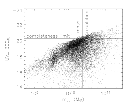
Figure 1: Absolute AB magnitudes of $z=3$ galaxies at rest-frame 1600 Å as a function of baryonic mass. The absolute magnitudes take into account dust absorption. The vertical line indicates our mass resolution, $M_{res}=2.2\ 10^{10}M_{\odot}$, above which our sample of galaxies is complete. The horizontal line represents our completeness limit in terms of magnitude so that galaxies brighter than $M_{AB}^{res}(1600)=-20.3$ also form a complete sample.

2.2.2 History resolution

A more subtle effect of resolution is that missing small structures means missing part of our halo merging histories. As a matter of fact, the impact on our modelled galaxies is twofold :

• we miss small galaxy mergers because galaxies close to the resolution limit are formed smoothly in haloes at the resolution limit, instead of assembled through mergers of smaller objects that would have populated smaller progenitor haloes;

• we cool too much gas in too short a time on new central galaxies in haloes at the resolution limit. Had we resolved their host halo merging histories, part of this cold gas would have been split between smaller progenitors at earlier times and partly processed into stars already.

However, the ’observational’ signature of this resolution effect (physical properties, luminosities of galaxies) tends to disappear after a while. In practice, a galaxy in our standard N-body simulation needs to evolve for about 1 Gyr before we can be sure that its properties have converged. This is irrelevant at $z=0$ (resp. $z=1$), where only 3 (resp. 69) out of 19,372 (resp. 19,257) galaxies above the formal resolution limit $M_{B}=-18.9$ (resp. $M_{B}=-20.2$) are younger than this threshold. However, it becomes problematic at $z=3$, when the age of the Universe is only a couple of gigayears old and roughly 75% of the galaxies are concerned. As a consequence, we introduce in the following study an additional free parameter that we call the maturity age $t_{mat}$, and we discard from our sample any LBG whose first progenitor is younger than $t_{mat}=1.1$ Gyr at the time when this LBG is identified as such. As the need for this kind of selection is one of the most important drawbacks of our study, section 3.2.2 justifies in detail our choice of maturity criterion.

2.3 A typical mock field

Because Lyman Break selection is by definition an observational selection, it is necessary to apply as similar as possible criteria to our modelled galaxies sample before attempting a thorough comparison with the data. We therefore used the momaf package to simulate light-cones from galics outputs, as described in the momaf paper (see also the galics/momaf web-page http://galics.iap.fr/). Basically, the method consists in tiling a time sequence of simulation boxes along a mock line of sight, and computing the apparent properties of galaxies from their positions in this cone-like geometry. It allows us to use as much of the spatial information contained in the N-body simulation as possible in order to produce realistic mock catalogues, which can then be analysed in the same way as real observations.

In Fig. 2, we show a typical result of this work : a mock medium deep field of $3\times 3$ arcmin² seen in the $R$ band (Steidel & Hamilton, 1993). The circles indicate LBGs, which are identified as indicated in section 3.1.

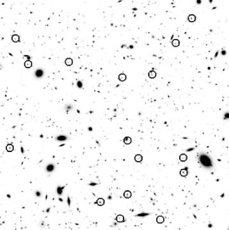
Figure 2: Mock medium deep field, of size $3\times 3$ arcmin², seen in the $R$ band. Circles mark the position of LBGs which were selected using the colour and apparent magnitude criteria given by Eq. 6.

3 LBG selection process

3.1 Colour-colour selection

It is the IGM extinction that makes the Lyman break selection such an efficient technique for selecting high-redshift galaxies. Galaxy evolution, along with dust absorption inside galaxies, also produce a Lyman-break, but its intensity varies from one galaxy to the next, so that galaxies end up scattered all over the colour-colour plane and as a result, colour and redshift would be strongly degenerate. Not only does the IGM attenuation yield a more pronounced Lyman-break, but the fact that it is due to material external to the galaxies makes this break independent from intrinsic properties of the observed objects, allowing the observer to select a whole population of “normal” galaxies at $z\sim 3$.

For a galaxy at this redshift, the Lyman break falls between the $U_{n}$ and $G$ filters (Steidel & Hamilton, 1993). It makes the $U_{n}-G$ colour of galaxies very sensitive to small variations of redshift around this value, as shown by the very steep slope in the colour-colour diagram of Fig. 3. This spread of the galaxy distribution along the $U_{n}-G$ axis leads to a precise selection of galaxies in redshift space. The colour criteria for selecting objects at $z\sim 3$ proposed by Steidel et al. (1995), which we adopt throughout this paper, is the following :

$$\begin{array}[]{lll}R&\leq&25.5\\ G-R&\leq&1.2\\ U_{n}-G&\geq&G-R+1\\ U_{n}-G&\geq&1.6\\ G-R&\geq&0.0.\end{array}$$ (6)

In Fig. 3, we show a colour-colour diagram for a mock catalogue of 360 arcmin². Only galaxies with an apparent AB magnitude lower than $25.5$ in the $R$ band are shown, in order to mimic the detection limit quoted by these authors. We represent galaxies which have redshifts between $2.7$ and $3.4$ as diamonds. Galaxies with other redshifts are marked as simple dots. The colour criterion given by Eq. 6 is shown as the solid line.

Notice that the distribution of galaxies in the colour-colour plane is smooth in Fig. 3. This behaviour stems from distributing galaxies in a mock light-cone, in contrast with previous studies based on pure semi-analytical models (Baugh et al. (1998), Somerville et al. (2001)), where galaxy properties were only computed for a discrete set of time outputs.

Figure 3: $(U_{n}-G)$-$(G-R)$ diagram, for a mock 360 arcmin² field. Only galaxies with apparent magnitude $R_{AB}\leq 25.5$ are shown. Diamonds represent galaxies that have their redshift in the range $[2.7;3.4]$, and points show galaxies out of this range. The solid contour shows the colour criteria for LBGs at $z\sim 3$ (Eqs. 6) , and the dashed contour shows our optimised contour for selecting galaxies at $z\sim 3$ (section 3.4). Notice the very steep rise in $U_{n}-G$ around $z\sim 3$, mainly due to the IGM attenuation. Photometric errors are not added in this plot.

3.2 Data sets

3.2.1 Observations

We choose to compare our modelled LBGs to the sample presented by Steidel and co-workers, for both the variety of results they have published so far (e.g. Giavalisco et al. (1998), Steidel et al. (1999), Shapley et al. (2001)), and the large number of sources it contains. The total area surveyed by these authors amounts to about a thousand arcmin², and contains $\sim$ 1250 LBG candidates (see Giavalisco et al. (1998), table 1, for a summary of observations). The density of observed LBGs on the sky is thus about 1.2 object per square arcminute, among which roughly 20% are estimated to be interlopers. Most of the observations were made using the three filters $U_{n}$, $G$, and $R$, designed to efficiently select objects at $z\sim 3$ (Steidel & Hamilton, 1993).

A point which is still unclear in the literature so far is the definition of interlopers. In principle, these are galaxies which, although selected by the colour criterion, are not at the requested redshift. In practise, it seems that the definition which is used by some authors is somewhat less strict, and objects are only called interlopers when they are galaxies at redshifts lower than $\sim 2.3$ or stars. We follow suit and adopt this broader definition but remark that since there are no foreground stars in our simulation, we do not expect to find many interlopers (see following section).

3.2.2 Simulations

We use the ($U_{n}$, $G$, $R$) filter set from Steidel & Hamilton (1993) to compute the apparent magnitudes of our simulated galaxies. Our standard mock catalogue size is 1 deg², and contains sources up to $z\sim 6.5$. We also use the same apparent magnitude detection limit, that is, $R\leq 25.5$.

As we discuss in momaf, a unique way to build a mock catalogue from the outputs of our simulation does not exist, because the mock light-cone intersects only fractions of each snapshot. We choose to introduce a random process in the generation of cones in order to be able to make independent realisations which are all a priori equally plausible. Because we do not include fluctuations on scales larger than the simulated volume, which is about 1 degree at $z\sim 3$, the dispersion of the number of LBGs found in different cones will yield an under-estimate of the cosmic variance on scales of one square degree (the size of our cones). We further point out that the mean LBG count derived from running a large number of realisation contains the full information available in the simulation.

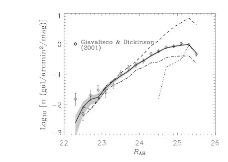
Figure 4: LBG counts from galics, compared to data from Giavalisco & Dickinson (2001) (diamonds with error bars). The solid line and grey area show the mean and 1-$\sigma$ region obtained from 20 mock catalogues of 1 square degree in which we applied the maturity age selection with $t_{mat}=1.1$Gyr. The dashed line shows the LBG number counts for a single cone, without any maturity selection, and the dot-dashed line shows the same counts with $t_{mat}=1.3$ Gyr. The dotted line shows counts from a higher resolution simulation covering a much smaller volume. Its normalisation justifies the value given to $t_{mat}$ (see text for discussion).

We ran 20 different light-cones, and found a mean number of LBGs $<N_{LBGs}>=4133$ per square degree, with a standard deviation of $\sigma_{N_{LBGs}}=183$. The modelled density of LBGs is thus $1.15$ arcmin^-2, consistent with the observed density of $1.22\pm 0.18$ arcmin^-2 (e.g. Giavalisco & Dickinson (2001)). In Fig. 4, we show the mean number counts, obtained from our 20 mock catalogues (solid line), as well as the dispersion, given at 1-$\sigma$ by the grey area. Our counts compare nicely with the data from Giavalisco & Dickinson (2001), over-plotted as diamonds. Note also that, as in real observations, we find very few interlopers (about 0.1%) with $z<2.3$. The dashed line shows counts for our modelled LBGs when we do not apply any maturity selection, and focus on a single example cone. The difference between these counts and the solid line shows that the history resolution mentioned in Sec. 2.2.2 mainly and strongly affects the faint end of the luminosity function (LF). Our most robust results thus concern the bright end of the modelled LBGs, where resolution does not affect galaxy properties. The dot-dashed line shows the counts for the LBGs which are older than 1.3 Gyr. The dotted line shows the counts obtained from a mock observing cone of 0.09 square degrees built with a higher-resolution $\Lambda$CDM simulation. This higher-resolution simulation contains $320^{3}$ particles in a cubic volume of side $32h^{-1}$Mpc. It has identical cosmological parameters as given in Sec. 2.1.1, and the galics post-processing was done using the same astrophysical parameter set as in galics i. The smaller volume and larger number of particles result in a galaxy mass resolution $M_{res}=3.77\times 10^{8}M_{\odot}$, i.e. $\sim 60$ times better resolution than in the fiducial simulation discussed here. As expected, the introduction of a maturity age $t_{mat}$ is irrelevant for the LBG counts of this high-resolution simulation. The faint-end normalisation of the counts supports our choice of $t_{mat}=1.1$ Gyr for our maturity criterion. The discrepancy in the bright counts are understood in terms of volume limit of the high-resolution simulation : just from Poisson statistics we expect about 30 times less objects per bin of luminosity since the volume is reduced by such a factor compared to the fiducial simulation. Furthermore, we have to account for cosmic variance which will affect more dramatically objects that are more clustered (see Sec. 3.5). Therefore, we cannot consider our high-resolution simulation as representative of the Universe as a whole, and for this reason, we prefer to use it only to fix the maturity criterion in the larger, low-resolution simulation, and we take this latter to make extensive predictions.

In the remainder of the paper, except where mentioned, we will use a single realisation of a mock catalogue. Since we have no information on how the data might be biased (cosmic variance), we can choose any of our available cones. We settle for one which contains $N_{LBGs}=4156$, in good agreement with the data, and close to our mean value.

3.3 Efficiency of the selection

Internal properties of galaxies are not fully eclipsed by the IGM attenuation, so one cannot expect to extract all the galaxies at a given redshift, and only these, from a simple region selection in the colour-colour plane. It is therefore interesting to define an efficiency of the selection process, which should account for the fraction of lost galaxies – that is, observable galaxies with the right redshift which do not meet the colour criteria – and the fraction of interlopers restricted here to galaxies lying outside the redshift range $[2.7;3.4]$. We therefore define the two following quantities:

• the completeness ($C$), which is the ratio of the number of selected galaxies with redshift $\sim 3$ to the number of detectable galaxies (i.e. galaxies with $R\leq 25.5$) at $z\sim 3$.

• the confirmation rate ($CR$) which is the ratio of the number of selected galaxies with $z\sim 3$ to the total number of selected galaxies (with any redshift).

With these two complementary quantities, we can define a measurement of the efficiency of a selection process as $E=C\times CR$. This quantity takes values from $0$ to $1$, $0$ meaning no source was detected at the expected redshift, and $1$ meaning that all the detectable sources with $z\in[2.7;3.4]$ were selected, and only these. For our sample of galaxies extracted from a 1 square degree field, we find the following values for the colour criteria given by Steidel and co-workers (eqs 6) : $C=96$%, $CR=88$%, and $E\sim 85$%. This high efficiency shows that the LBG selection is indeed a very good method for selecting distant galaxies, and the high completeness shows that this selection grabs 96% of the detectable galaxies at $z\sim 3$.

In an attempt to mimic observations, we also added photometric errors to our magnitudes. These are simply modelled here as uniformly-distributed random values, between $\pm\delta$ mag, in the three bands $U,G,R$. The selection efficiency drops to $E=70\%$ when $\delta$ reaches $0.25$ mags. For a more conservative error amplitude of $0.1$ magnitude, the efficiency settles around $80$%. Obviously, photometric errors are far more complex than this simple model and should take into account systematics. Nevertheless, their impact on LBG selection as assessed by our simple estimate constitutes a useful first estimate.

3.4 New contour

Until now, the colour selection used to select distant galaxies from multi-band imaging observations has been defined by placing synthetic galaxies, with a ’wide range’ of ages, star formation histories, metallicities, dust content and redshifts (e.g. Steidel et al. (1995), Madau et al. (1996)), onto a colour-colour plane, and by finding out which region encloses most distant galaxies and fewest interlopers. This method, although spectroscopic follow-up showed it gives good results, sweeps under the carpet the question of the nature of the distant objects. It is expected to be robust anyway since IGM extinction –which is external to galaxies– plays a dominant role in the location of galaxies in the colour-colour plane. However, one might wonder whether a tighter set of criteria could be found if the ’wide range’ of properties was replaced by more ’plausible’ properties for galaxies at a given redshift. We present here the first attempt to build such criteria with an ab initio model of galaxy formation, in which distant galaxies’ properties come out naturally of the hierarchical evolution within the dark matter content of the universe.

We found our best contour in the colour-colour plane using the downhill simplex method (Press et al., 1992) in order to maximise the efficiency of the LBG-selection for a pentagonal contour with two sides bound to be vertical, and one horizontal in the $(U_{n}-G;G-R)$ plane. For this maximisation, we used our full fiducial catalogue of one square degree so as to have a significant number of LBGs. The contour we calculate is the following :

$$U_{n}-G \geq 1.7,$$

$$G-R \geq -0.2,$$

$$G-R \leq 1.9,$$

$$U_{n}-G \geq 0.9(G-R)+1.1,$$

$$U_{n}-G \leq 0.6(G-R)+5.1.$$

This contour (the dashed lines of Fig. 3) gives an efficiency $E=88$%, instead of $E=85$% for the contour defined by Eq 6. Our efficiency is higher because we discard a large fraction of high-$z$ interlopers by setting an upper limit on the $U_{n}-G$ colour, which increases our confirmation rate to $CR=95$%. However, our contour decreases the completeness ($C=94$%), precisely because of this more accurate selection. In practise, the aim of LBG surveys is twofold : (i) select a large number of high-$z$ candidates, with redshifts as high as possible, allowing for a broad redshift range, and (ii) use the detected galaxies to describe the properties of ’normal’ galaxies at a given redshift. In case (i), one wishes to favour completeness relative to confirmation rate. In the second case, one wishes to reach a compromise between $C$ and $CR$. Bearing this in mind, it is worth pointing out that our selection is quite similar to that used by Steidel and collaborators. This gives the overall impression that the UV-dropout technique is quite robust, and independent of stellar population modelling. As mentioned earlier, this robustness was expected since the locus of galaxies in the colour-colour plane is mainly given by IGM absorption, and thus by redshift.

3.5 Cosmic variance

LBGs	4 arcmin2	16 arcmin2	64 arcmin2	400 arcmin2	1600 arcmin2
	$<N>$ ($\sigma_{N}$)	$<N>$ ($\sigma_{N}$)	$<N>$ ($\sigma_{N}$)	$<N>$ ($\sigma_{N}$)	$<N>$ ($\sigma_{N}$)
$R\leq 25.5$	4.62 (2.76)	18.35 (7.07)	73.00 (18.9)	454.6 (66.9)	1817 (154)
$R\leq 25.$	2.71 (1.94)	10.74 (4.80)	42.74 (12.2)	266.1 (42.1)	1064 (93.9)
$R\leq 24.5$	1.21 (1.20)	4.78 (2.74)	19.04 (6.69)	118.3 (21.4)	473.1 (46.6)

Table 1: Mean expected numbers of LBGs brighter than $R=25.5$, $25$ and $24.5$, in fields of 4, 16, 64, 400 and 1600 arcmin². The standard deviations are also given between brackets. These standard deviations are systematically higher than the square-root of the number of sources, because of the strong effect of clustering.

The degree to which observations of small areas are representative of the whole Universe is a crucial question when one wishes to interpret data in the cosmological context. Since our model contains spatial information, it is possible to study the cosmic variance of LBG densities, at least to a certain extent, because our simulation is volume-limited and does not include long-wavelength fluctuations.

We estimated the cosmic variance as the field-to-field variation in the number of LBGs in sub-fields, extracted from our 20 different 1 deg² fields. For each size of sub-fields, ranging from 4 arcmin² to 1600 arcmin², we used 20000 random sub-catalogues (1000 per 1 deg² mock catalogue) to estimate the mean number of LBGs and the associated variance.

In table 1 we give the mean numbers of LBGs and the corresponding standard deviations for fields of 4, 16, 64,400 and 1600 arcmin². Numbers are given as well for LBGs brighter than $R=25$ and $R=24.5$. The fact that the standard deviation is higher by a factor $>2$ to the poissonian deviation is a direct signature of the high clustering properties of LBGs.

In Fig. 5 we show the variation of the relative deviation ($\sigma/\langle N\rangle$) versus the surface of the mock survey. The continuous line shows the measured deviation and the dotted line shows the Poissonian prediction. The dashed line shows the quadratic difference between those : $\sigma_{c}/\langle N\rangle=(\sigma^{2}_{N}-\sigma^{2}_{Poisson})^{1/2}/\langle N\rangle$, where $\sigma_{c}$ is the contribution of clustering to the cosmic variance. The three crosses at 3600 arcmin² show the total dispersion and the contributions of clustering and Poisson, from top to bottom. These were estimated only from our 20 mock catalogues and thus rely on less statistics than the curves. On small scales ($<7$ arcmin²), where the sources are rare enough, the Poissonian noise dominates the variance. On larger scales, the variance is dominated by the clustering of LBGs, as the Poissonian variance falls off more rapidly. As the Universe is homogeneous on large scales, we expect the clustering contribution to dwindle progressively as the size of the survey increases. This regime is however out of reach with our current simulation because the simulated volume has an angular size of $\sim 1$ square degree at $z\sim 3$. Above this scale we are bound to under-estimate the dispersion. Because of this, we cannot tell at the moment whether the points at 3600 arcmin² in Fig. 5 are low due to finite volume effect or to the fact that we reached the point where clustering strength starts to vanish.

Figure 5: Standard deviation in number counts of LBGs as a function of the survey area in square arcminutes. The solid curve is the measured standard deviation, and the dotted one is the Poissonian prediction. The dashed curve shows the quadratic difference between the measured deviation and the Poissonian one, namely, the contribution of clustering to the cosmic variance.

4 Clustering

The clustering properties of LBGs give important constraints on the dynamical processes that drive galaxy formation. Moreover, they can be observed directly and no assumptions are necessary to compute the angular correlation function. In this section, we show different aspects of the clustering properties of our modelled LBGs, namely, halo masses, the location of LBGs in the cosmological simulation, the angular correlation function, the spatial correlation function, and the bias of LBGs relative to dark matter.

4.1 Halo masses

A first impression of the clustering properties of LBGs can be given by the mass distribution of the dark matter haloes which harbour them. In Fig. 6, we show the masses of these haloes versus the redshifts at which the LBGs are detected in our simulation. The median halo mass for our LBGs is $15.8\times 10^{11}M_{\odot}$, as indicated by the horizontal dotted line. This mass is about ten times the halo mass resolution of the simulation. The median values for populations of modelled LBGs with various luminosities are given in table 2. The relatively large mass of the haloes harbouring our modelled LBGs at $z\sim 3$ indicates that these galaxies are highly biased with respect to the dark matter distribution. This matches qualitatively what is observed in different surveys (Giavalisco et al. (1998), Arnouts et al. (2002)).

Figure 6: Masses of LBG host haloes as a function of redshift. The horizontal dotted line shows the median mass value of $\sim 16$ $10^{11}M_{\odot}$.

LBGs	$<M_{halo}>$
	($10^{11}M_{\odot}$)
$R\leq 25.5$	15.8
$R\leq 25$	15.4
$R\leq 24.5$	14.0

Table 2: Median masses of DM haloes harbouring LBGs.

4.2 Location of LBGs and their descendants

On the left-hand side panel of Fig. 7, we show the location of LBGs at $z\sim 3$ in a slice of our simulated cosmological volume. The white discs show LBGs, and the underlying grey background shows the dark matter density (the darker the denser), in logarithmic scale. The LBGs are clearly highly clustered in this picture. The right-hand panel shows the location of the descendants of LBGs at $z=0$ as squares. Black squares indicating spiral galaxies, and white squares elliptical or lenticular galaxies. The white discs are elliptical/lenticular galaxies which do not have a LBG progenitor at $z\sim 3$. The descendants of LBGs are even more highly clustered than LBGs themselves, as they fell into DM structures from $z=3$ to $z=0$. We will come back to the properties of the descendants of LBGs in section 6.2.

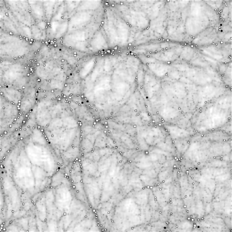
Figure 7: Left hand panel : location of LBGs at z=3. White discs show LBGs, and the DM density (in log) is shown in grey scale, the darker the denser. Right hand panel : location of local ellipticals and the descendants of LBGs in the same comoving volume, at redshift 0. The white symbols show elliptical or lenticular galaxies, the squares indicate descendants of LBGs that are present in the volume of the left hand side panel. Black squares show spiral descendants of LBGs. The LBGs and their descendants are highly clustered, located in dense DM regions. The projected volume shown is 150 Mpc on a side, and has a depth of 15 Mpc.

4.3 Angular correlation function

For the computation of the angular correlation function (ACF), we used the estimator proposed by Landy & Szalay (1993) (hereafter LS93) :

$$w(\theta)=\frac{DD(\theta)-2DR(\theta)+RR(\theta)}{RR(\theta)},$$ (7)

where $DD(\theta)$ is the number of pairs of LBGs with angular separation between $\theta$ and $\theta+\delta\theta$, $RR(\theta)$ is the analogous quantity for a random catalogue, and $DR(\theta)$ the number of observed-random pairs.

The estimate of the errors in the general case is a difficult task. Here, we consider Poissonian noise (in the number of pairs) only. We expect this to be a good approximation because our survey is large enough (compared to the scales we probe), and we deal with a rather diluted distribution of galaxies so that finite-volume errors will be negligible compared to discreteness errors. Moreover, considering only Poissonian error-bars implies that we underestimate the real uncertainties. It is not a concern here as our goal is to show that our spatial distribution of LBGs is consistent with the observed one – and this is the case within Poissonian uncertainties (see next section). Following LS93, we write Poissonian errors as :

$$\sigma_{w}(\theta)=\frac{1+w(\theta)}{\sqrt{N_{g}(N_{g}-1)}}\left[\frac{N_{r}(N_{r}-1)}{RR}\right]^{1/2},$$ (8)

where $N_{g}$ is the number of galaxies in our mock survey, and $N_{r}$ the number of objects in our random catalogue (here, $N_{r}\sim 7\times 10^{4}$). The first factor in the above equation shows the Poissonian contribution, as it is inversely proportional to the square root of the number of LBG pairs. The second term is a geometrical contribution, and depends only on the shape of the survey. In this expression of the standard deviation, we have assumed that the integral constraint was negligible. Of course, the standard deviation of Eq. 8 strongly depends on the angular bin-size we use to evaluate the ACF. This appears only implicitly : if the bin size doubles, RR will also roughly double, and so $\sigma_{w}$ will be divided by a factor $\sqrt{2}$. In order to compare our results to those of Giavalisco et al. (1998), we adopt the same binning as these authors.

Finally, note that the random transverse shifting of boxes every 150 comoving Mpc along the line of sight that we use to suppress replication effects implies an underestimate of the ACF of about 10% at most, as detailed in momaf.

Our measured ACF is represented in Fig. 8, by crosses and their error-bars. The solid line shows a maximum likely-hood fit of a power-law $w(\theta)=A_{w}\theta^{-\beta}$ to our data. The best fit parameters are : $A_{w}=4.41\pm 0.78$ and $\beta=0.9\pm 0.04$. This is consistent with the results from Giavalisco et al. (1998). Their fit to observed data is shown in Fig. 8 by the shaded region. The vertical dotted line roughly shows the angular size of a cluster of galaxies at $z\sim 3$, below which the contribution to clustering mainly comes from pairs of galaxies within the same halos. In galics, the positions of galaxies inside halos are given according to some prescription and not directly measured from the N-body simulation. Hence our model only makes reliable predictions for the two-halos contribution to $w(\theta)$.

Figure 8: Angular correlation function for our sample of LBGs, extracted from a 1 square degree mock catalogue. The crosses show our estimate of $w(\theta)$ with the LS93 estimator, and the error bars come from a Poissonian estimate. The grey area shows data from Giavalisco et al. (1998). This area corresponds to their “LS-random” estimate, which is similar to ours. The solid line shows a maximum-likelihood fit to our data by a function $w(\theta)=A_{w}\theta^{-\beta}$, with best fit values indicated in the panel.

4.4 Spatial correlation function and linear bias

We computed the spatial correlation function (SCF) using the same estimator (LS93) as for the ACF. This time, however, we computed the SCF directly from the snapshots of galics, bypassing the cone of sight generation. We show the result in Fig. 9. The top panel is the SCF of LBGs identified in the snapshot at $z=3$. The error bars only show the poissonian deviations. The bottom panel shows the linear bias of LBGs relative to the dark matter particles of the cosmological N-body simulation ($b^{2}(r)=\xi_{LBG}(r)/\xi_{DM}(r)$). We limit our plots to the approximate range 1-10 $h^{-1}$Mpc for two reasons : (i) we distribute galaxies inside clusters according to a semi-analytic spherically symmetric prescription, so we loose angular information for some galaxies below 1 $h^{-1}$Mpc, and (ii) to avoid edge effects, we limit the study to scales below one tenth of the simulated volume size (100 $h^{-1}$Mpc).

Figure 9: Top panel : spatial correlation function of our modelled LBGs in the snapshot corresponding to z=3. Bottom panel : linear bias of our modelled LBGs with respect to the dark matter.

We find that the linear bias slowly decreases from $\sim 5$ to $\sim 3$ between 0.5 and 20 comoving $h^{-1}$Mpc. This is compatible with the bias estimated by Giavalisco et al. (1998), Adelberger et al. (1998) and Porciani & Giavalisco (2002).

5 UV/IR luminosity budget

One of the most important challenges toward understanding galaxy formation is to determine at which epoch stars formed, or, in other words, how and when did the mass of stars we see in local Universe galaxies assemble. The observation of distant galaxies in the optical window is now known to be insufficient to retrieve star formation rates (e.g. Devriendt et al. (1999)). The discovery of the cosmic far infrared background, and the numerous IR/sub-mm surveys, have made it clear that dust extinction within galaxies plays a fundamental role in determining the UV emission of distant galaxies, and therefore in extracting information on the cosmic star formation rate. The reason is that the UV luminosity of a galaxy is governed by the amount of recent star formation –which is responsible for young massive stars dominating the energetic part of the SED– and dust absorption –which is most efficient at UV wavelengths, and re-emits light in the IR/sub-mm domain. Unfortunately, far infrared or sub-mm instruments do not yet have sensitivity or resolution which would make a thorough follow-up of LBGs at large wavelengths possible.

Our model includes a treatment for dust extinction and emission in the IR/sub-mm domains, which allows us to predict extinction properties of LBGs, and make the connection between LBGs, seen in the optical, and sources detected at IR/sub-mm wavelengths. In this section, we first discuss the UV luminosity function and selection effects. Second, we consider the extinction properties of these objects as predicted by galics. Third, we show how both effects alter the so–called Madau diagram (Madau et al., 1996). We eventually make predictions concerning the detectability of the sub-mm counterparts of LBGs.

5.1 Luminosity functions at $z\sim 3$

Figure 10: Luminosity functions at $z\sim 3$, for LBGs. The x-axis shows absolute $R$ magnitudes in the observer frame. The black diamonds show the data from Steidel et al. (1999), converted to the current cosmology. The solid histogram shows the LF we compute for our sample of LBGs, using the effective volumes given in Steidel et al. (1999). We assume a single luminosity distance for the whole sample (also given by Steidel et al. (1999)). This histogram is in fair agreement with the data. The dashed histogram shows the LF computed for all the detectable galaxies (i.e. galaxies with $R\leq 25.5$) in our sample that have a redshift between $2.7$ and $3.4$. Here, we normalised the LF to the total volume of the cone of sight between redshifts 2.7 and 3.4. We also used the “true” luminosity distance of each galaxy. This LF is lower than the previous one because of volume corrections. Finally the dotted histogram shows the true luminosity function of LBGs only, i.e. without volume corrections. The two vertical dotted lines show the resolution and detection limits.

In Fig. 10, we compare different estimates of our measured luminosity function (LF) at $z\sim 3$ with the LF given by Steidel et al. (1999).

• The solid histogram shows the LF for all our modelled LBGs, computed in the same way Steidel et al. (1999) computed their observed LF. First we divide the number of LBGs in each apparent-magnitude bin by the effective volumes quoted by these authors for our cosmological parameters. Then, we convert our apparent magnitudes to absolute magnitudes using the relation $L_{\nu}=10^{-0.4(48.6+m_{AB})}\times 4\pi d_{L}^{2}/(1+z)$ where $d_{L}=5.6\ 10^{28}\ h^{-1}$cm, is the single value of the luminosity distance given by Steidel et al. (1999) for $z=3.04$ in a $\Lambda$CDM universe ($\Omega_{\Lambda}=0.7$, and $\Omega_{m}=0.3$). Note that the difference in luminosities induced by using a single redshift and luminosity distance are negligible when compared to the uncertainties in the volume corrections.

• The dashed histogram shows the luminosity function of all detectable galaxies ($R\leq 25.5$) with redshifts between 2.7 and 3.4. This time, we first convert apparent magnitudes to absolute magnitudes using each galaxy’s luminosity distance and redshift. We then divide the number of objects in each magnitude bin by the total volume of the cone of sight between $z=2.7$ and $z=3.4$, ignoring any volume effect due to the selection function.

• The dotted histogram is the same as the previous one, but only includes LBGs. It lies just below the dashed histogram in every bin, showing that LBG selection is more or less equally efficient at all magnitudes.

The resolution and detection limits are shown as dotted vertical lines. The former limit was defined in section 2.2. The latter is given by Steidel et al. (1999) and corresponds to the apparent magnitude limit $R\leq 25.5$. Our resolution limit is of the same order.

The solid curve of Fig. 10, which reproduces the analysis of Steidel et al. (1999), yields a very encouraging match to the data. At this stage, we remind the reader that in this paper we use the same galics  model that was used in galics i  to reproduce local galaxy properties. It is therefore an impressive result that we manage to match the observed luminosity function (or the number counts shown in Fig. 4) of galaxies at high redshift as well.

Figure 11: Effect of dust extinction on the luminosity function of galaxies at $z\sim 3$. The solid histogram shows the LF of all our modelled LBGs at $z\sim 3$, as a function of their apparent $R$ magnitudes. The dashed histogram is the LF these galaxies would have if they contained no dust. It was computed directly from the rest-frame emission of galaxies at 1600Å, assuming no extinction. Finally the dotted histogram presents the same results as the dashed one but shifted by 2 magnitudes to facilitate comparison with the solid histogram.

In Fig. 11, we show the effect of dust extinction on luminosity functions. The solid histogram on this figure represents the absolute $R$ magnitude (in the observer frame) luminosity function, and includes all our modelled galaxies at $z\sim 3$ (with the usual $R\leq 25.5$ criterion on apparent magnitude). The dashed histogram corresponds to the luminosity function of all these galaxies computed directly from their luminosities at 1600Å in the rest-frame, assuming no extinction. The dotted histogram is the dashed one shifted two magnitudes fainter to facilitate the comparison with the extinguished LF (solid histogram). Note that the filters differ for the two LFs. Indeed, the $R$ filter blue-shifted to $z\sim 3$ has a width $\Delta\lambda\sim 375$Å and is centred at $\lambda_{R}\sim 1700$Å, whereas the filter we used to compute the 1600Å emission is centred at this wavelength (in the galaxy rest-frame), and is a top-hat function of width 20Å. Nevertheless the huge difference between the two histograms demonstrates how delicate it is to extract the UV flux really emitted from observed broad band fluxes. We emphasise that it is this very same UV flux which is mainly used to compute the cosmic star formation rate at intermediate and high redshift. Moreover, as a final note of caution, we stress that even the slopes of the LFs differ, which means that a unique conversion factor in not sufficient to accurately correct data for extinction.

5.2 Extinction of LBGs

Obscuration by dust plays a key role for the extraction of star formation rates from UV observations. Here, we show how LBGs and other detectable galaxies at $z\sim 3$ are affected by this process, and we give the mean extinction factors predicted by galics for these galaxies.

5.2.1 Qualitative view

Figure 12: Ratio of IR luminosity (8$\mu$m $<\lambda<$ 1000 $\mu$m) to bolometric luminosity for LBGs (dots) and detectable galaxies with $z\in[2.7;3.4]$ (crosses) that do not meet the LBG selection criteria. Most of these galaxies emit more than half their light in the IR/sub-mm.

In Fig. 12 we show an estimate of the internal extinction versus redshift for our sample of LBGs and other galaxies at $z\sim 3$ which are brighter than $R=25.5$ (the so-called ‘detectable’ galaxies). Internal extinction is estimated here as the ratio of infrared bolometric luminosity (integrated from 8$\mu$m to 1000$\mu$m at rest) to bolometric luminosity. A value of 0.5 of this ratio means that half the light emitted by stars is absorbed and re-emitted by dust. We find that $\sim$95% of our LBGs emit more than half their light in the IR/sub-mm. This fraction of heavily extinguished objects holds for all detectable galaxies at $z\sim 3$. This suggests that an important contribution of the IR/submm background is due to $z\sim 3$ galaxies.

The fact that missed galaxies (crosses in Fig. 12) lie on rather narrow redshift bands on either side of $z\sim 3$ is another manifestation of the LBG selection efficiency: foreground galaxies are only missed because of border effects in the colour-colour plane, whereas background galaxies are more extinguished on average.

5.2.2 Extinction factor

The usual way to quantify extinction is through the absorption coefficient $A(\lambda)=k(\lambda)E(B-V)$, where $k(\lambda)$ is the adopted attenuation law. In terms of luminosities, this coefficient can be written as

$$A(\lambda)=2.5\log\frac{L_{no\ ext}(\lambda)}{L_{ext}(\lambda)},$$ (9)

where $L_{no\ ext}(\lambda)$ is the non-extinguished luminosity at wavelength $\lambda$, and $L_{ext}(\lambda)$ the extinguished one, computed for a given inclination of the galaxy. The extinction factor is then defined by $F(\lambda)=10^{0.4A(\lambda)}$, that is, in terms of luminosities, $F(\lambda)=L_{no\ ext}(\lambda)/L_{ext}(\lambda)$. This quantity is of great importance because it is necessary for the extraction of information about the star formation rates of distant galaxies. However, its value is still a matter of debate. This is partly due to averaging effects, as emphasised by Massarotti et al. (2001). Indeed these authors stress that computing an average extinction factor from an average absorption coefficient – namely

$$F_{ave}(\lambda)=10^{0.4\sum_{i}A_{i}(\lambda)/N}=10^{0.4<A(\lambda)>},$$ (10)

where $N$ is the number of galaxies in the sample – leads to an underestimate of the effect of dust. They suggest that one should rather use an effective extinction factor defined by

$$F_{eff}(\lambda)=\frac{1}{N}\sum_{i}10^{0.4A_{i}(\lambda)}=10^{0.4A_{eff}(\lambda)}.$$ (11)

In order to understand the difference between both estimates, it is easier to re-write them in terms of luminosities. The average extinction factor becomes the geometric mean

$$F_{ave}(\lambda)=\left[\prod_{i}\frac{L_{no\ ext}^{i}(\lambda)}{L_{ext}^{i}(\lambda)}\right]^{1/N},$$ (12)

whereas the effective extinction factor is simply the arithmetic mean

$$F_{eff}(\lambda)=\frac{1}{N}\sum_{i}\frac{L_{no\ ext}^{i}(\lambda)}{L_{ext}^{i}(\lambda)}.$$ (13)

We have computed both factors for our modelled galaxies, in order to facilitate the comparison with Steidel et al. (1999) who use $F_{ave}(1600)=4.7$, and also to see whether they give us results which differ by a factor $\sim$ 3, as claimed by Massarotti et al. (2001). We summarise our results in table 3. We only find a discrepancy of about a factor 1.3 between the two estimators, with extinction factors $F_{eff}\sim 6.2$ and $F_{ave}\sim 4.75$. These values are much lower than the value of 12$\pm$2 obtained by Massarroti and co-workers, but their analysis is based on the Hubble Deep Field only, and includes galaxies spanning a much wider range of redshifts than those we consider here. Our average extinction factor has a value close to that used by Steidel et al. (1999), and our effective extinction factor is consistent with the detailed analysis of Adelberger & Steidel (2000) who conclude the effective extinction should be around a factor $\sim 8$.

LBGs	$F_{eff}(1600)$	$F_{ave}(1600)$
$R\leq 25.5$	6.19	4.75
$R\leq 25$	6.13	4.67
$R\leq 24.5$	6.21	4.83

Table 3: Extinction factors at 1600 Å for different sub-populations of modelled LBGs. The two estimators described by Massarotti et al (2001) are given for each sub-sample.

5.3 Cosmic star formation rate

Another uncertain step in retrieving star formation rates from UV fluxes is the UV-SFR connection, considering no absorption (or no dust). This relation is quite sensitive to the initial mass function (IMF) and we remind the reader that the IMF in this analysis is the same we used in our fiducial model described in galics i, namely a Kennicutt (1983) IMF from 0.1 M_⊙ to 120 M_⊙.

5.3.1 UV/SFR conversion

The first step is to obtain extinction factors, in order to relate the observed magnitudes to the UV flux that galaxies emit prior to extinction. The second step is to make the link between these extinction-corrected UV luminosities and star formation rates. This effectively is feasible because massive stars are the main contributors to the galaxy UV flux and are sufficiently short-lived. However, star formation rates have to be averaged over a period of about 100 Myr so that a robust enough relation may be establish (e.g. Kennicutt (1998)). In table 4 we give SFR-to-UV luminosity ratios for different sub-populations of LBGs, whose SFRs are evaluated as the mass of stars younger than 100 Myr, divided by that period of time. Because of the rapid timescale of stellar evolution, this is an under-estimate of the real SFR, by about 20% for Kennicutt IMF. We also give ratios computed using the instantaneous SFR for comparison. Both these estimates yield reasonable values because the evolution of the SFR is generally small over a 100 Myr period and therefore are consistent with Madau et al. (1996) – who use a conversion factor of $9.54$ M_⊙ yr^-1 per $10^{29}$erg s^-1 Hz^-1– and with Kennicutt (1998), who gives a value of $14$ M_⊙ yr^-1 per $10^{29}$erg s^-1 Hz^-1. The ratios we compute, however, are the result of particular star formation histories: those of our LBGs. Looking at table 4, one remarks that averaged SFRs are systematically larger than their instantaneous counterparts by about a factor two. This indicates that modelled LBGs tend to be identified as such when they enter a “post-starburst” phase.

LBGs	SFR${}_{100}/$ L(1600)	SFR${}_{inst}/$ L(1600)
$R\leq 25.5$	16.7 (3.3)	8.94 (2.2)
$R\leq 25$	16.8 (3.6)	8.88 (1.1)
$R\leq 24.5$	16.8 (4.5)	8.77 (0.9)

Table 4: SFR to UV luminosity ratios (in M_⊙ yr^-1 per $10^{29}$erg s^-1 Hz^-1) computed for different subsamples of our modelled LBGs. The UV luminosities are computed as if the galaxies contained no dust, that is, with no extinction. In the first column, the SFR is computed as the mass of stars younger than 100 Myr divided by 100 Myr. In the second column, the SFR is the instantaneous star formation rate, computed over a Myr only. For sake of completeness we also give standard deviations between brackets for each sub-class of LBGs.

5.3.2 The cosmic star formation rate history

Following Steidel et al. (1999), we compute the cosmic SFR at $z\sim 3$ from our UV luminosity function. Integrating the modelled UV LF of LBGs and converting it into a star formation rate density using Table 4, we find $\rho_{SFR}=8.9\times 10^{-3}$ M_⊙yr^-1Mpc^-3. Correcting this value for extinction with the effective factor of Table 3 yields a density $\rho_{SFR}=5.5\times 10^{-2}$ M_⊙yr^-1Mpc^-3. The last step is to correct for the missing faint end of the luminosity function (unresolved galaxies). Following Steidel et al. (1999), we apply a correction of 0.5 dex and find $\rho_{SFR}=0.17$ M_⊙yr^-1Mpc^-3, which is consistent with Steidel et al. (1999) and Adelberger & Steidel (2000).

5.4 Prediction of sub-mm flux

One of the main ambitions and major difficulties of hierarchical models of galaxy formation is to reproduce the sub-mm number counts. Several attempts have been made in semi-analytic models to fit these observations, but none of the recipes has yet emerged as a well accepted solution. Guiderdoni et al. (1998) implemented a massive IMF to obtain SCUBA objects, but there is neither a real physical motivation for this solution, nor strong observational hints. Devriendt & Guiderdoni (2000) introduced an ad-hoc redshift evolution which did not possess firmer foundations. Finally, Balland et al. (2003) used a simple yet physically motivated model to estimate energy exchanges during galaxy interactions which they propose as the principal mechanism for triggering starbursts. They show that this solution yields a good match to mid-IR as well as SCUBA counts. A thorough discussion on this topic will be given in paper 4, but we forewarn the reader that the fiducial galics model presented in galics i that we are using for the present study probably underestimates the cosmic amount of 850 $\mu$m light by a factor $\sim$2.

In Fig. 13 we show ratios of IR to UV (1600Å) luminosities versus the sum of these luminosities for our modelled LBGs. As a crude approximation, this is equivalent to “dust absorption” versus “star formation rate”. The grey regions broadly indicate the contour of the data analysed by Adelberger & Steidel (2000), and the solid line shows the SCUBA detection limit. The good match between observations and our modelled LBGs suggests that we manage to compute dust absorption and star formation rates in a consistent way. We also recover the observed correlation between star formation and dust content of the galaxies : the more obscured, the more star-forming. However, we predict that only about 1 % of our modelled LBGs should be detectable with SCUBA at 850 $\mu$m at the 2 mJy level, in agreement with the estimates of Chapman et al. (2000).

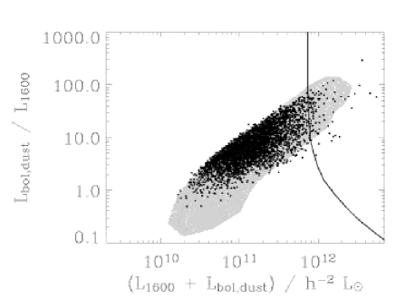
Figure 13: Ratio of IR to 1600Å luminosity versus the sum of these luminosities. In a first approximation, this shows absorption by dust versus star formation rate. The grey region roughly indicates the location of observed LBGs (Adelberger & Steidel, 2000), whereas the dots represent our modelled LBGs. The solid line marks the SCUBA detection limit at 850 $\mu$m.

The model can be used to make predictions for other IR/submm surveys. For instance, we find that the SWIRE survey with SIRTF will be able to detect only 0.04% (resp. 0%, 0%, 0%, 0.02%, 1.4%, 2.3%) of them at 170 $\mu$m (resp. 70$\mu$m, 24$\mu$m, 8$\mu$m, 5.8$\mu$m,4.5$\mu$m, 3.6$\mu$m) at the 17.5 mJy level (resp. 2.75mJy, 0.45mJy, 32.5$\mu$Jy, 27.5$\mu$Jy, 9.7,$\mu$Jy 7.3$\mu$Jy). These objects are clearly a key target for ALMA which should be able to detect all of them at 850 $\mu$m or $1.3$ mm, at the 0.1 mJy level.

Predictions at other optical and IR/submm wavelengths can be easily retrieved from queries to our web interfaced relational database located at http://galics.iap.fr.

6 Nature of LBGs

As emphasised by Shapley et al. (2001), the question of the nature of LBGs remains quite open. Different models suggest that LBGs are seen because they are undergoing strong starbursts due to major mergers, whereas others claim that LBGs are central galaxies of massive haloes that form stars steadily so as to reach a consequent size by redshift 3. The increasing number of observations seems to indicate that LBGs have many facets. Each of the two above-mentioned scenarios can explain some of their properties. We describe in this section the general properties of our modelled LBGs and investigate their star formation histories.

6.1 Physical properties

Figure 14: Top left panel : Radius (kpc) distribution for our modelled LBGs. The radius is a stellar-mass weighted average radius of three components: disc, bulge and starburst. The median value of $\sim 2.6$ kpc, indicated with the dotted vertical line, is in good agreement with the data from the HDF (Giavalisco et al., 1996). Top right panel : Stellar mass distributions for our modelled LBGs. The median value of $2.6\times 10^{10}$M_⊙ is indicated by the dotted vertical line. Bottom left panel : The solid histogram shows the 3-component average ISM metallicity distribution of our modelled galaxies, the dotted histogram that of the discs, the dashed histogram that of the bulges and the dot-dashed one that of the starbursts. Bottom right panel : The solid histograms represent the distribution of instantaneous SFRs of our modelled LBGs, whereas the dotted histogram shows the distribution of SFRs averaged over 100 Myr for the same galaxies. The median SFR_inst is $\sim$28 M_⊙ yr^-1, as indicated by the left hand side vertical dotted line, and the median of SFR₁₀₀ is $\sim$50.8 M_⊙ yr^-1, indicated by the right hand side vertical dotted line.

Sizes

In Fig. 14 we show the distribution of sizes of our modelled LBGs. The size of a galaxy is defined here as the stellar-mass weighted average of the three component (disc, bulge, starburst) half-mass radii. We find a median value of $2.6$ kpc for our LBGs, which is in good agreement with the analysis by Giavalisco et al. (1996) of a few LBGs observed with the HST (but identified with ground-based images) for which they find a typical size of about $2$ kpc. The mean values and standard deviations are summarised in table 5.

Stellar masses

The distribution of stellar masses of our modelled LBGs is given in Fig. 14. The median stellar mass is $2.6\times 10^{10}$ M_⊙, in very good agreement with the mean stellar mass deduced from data by Shapley et al. (2001) ($<M_{star}>_{med}=2.4\times 10^{10}$ M_⊙), and Papovich et al. (2001) ($\sim 10^{10}$ M_⊙). The shape of our distribution is consistent with that given by Shapley et al. (2001, their Fig. 10b), and also with the “accelerated quiescent” model of SPF (Primack et al., 2001).

Metallicity

The distribution of metallicities of our modelled LBGs is given in Fig. 14. The solid histogram shows the 3-component average ISM metallicity of our modelled galaxies, the dotted histogram that of the discs, the dashed line shows that of the bulges and the dot-dashed one that of the starbursts. We find a median metallicity of about $Z_{\odot}/5$, which is again in good agreement with observations (Pettini et al., 2001). The starburst and bulge components have higher metallicities, due to the more intensive star formation taking place there.

Star formation rates

In Fig. 14 we show the distribution of star formation rates (SFR) for our modelled LBGs computed in two different ways. The solid line shows the instantaneous star formation rate (SFR_inst), computed over the last Myr. This quantity is not directly comparable to the value deduced from observations of the UV through broad band filters (see discussion in Kennicutt (1998)). However, they indicate the current state of LBGs, and should compare better to estimates of SFR obtained from emission lines. For this estimate, we find a median value of 27.4 M_⊙ yr^-1, lower than the observed value by a factor $\sim 3$. The dotted curve shows the distribution of star formation rates computed as the mass of stars younger than 100 Myr, divided by 100 Myr (SFR₁₀₀). This is much closer to what is deduced from observations by Shapley et al. (2001) as it takes into account the star formation history during a time of order the lifetime of B and A stars. Our measure is however an under-estimate of the real SFR (by about 20%) because we miss all the mass lost through stellar evolution during a 100 Myr. The median value of SFR₁₀₀ is 50.8 M_⊙ yr^-1, with 20% of the modelled LBGs forming more that 100 M_⊙ per year. These SFRs are in better agreement with the data, although still low compared to the estimate of Shapley et al. (2001) : $\sim 90$ M_⊙ yr^-1.

The question of what triggers these high SFRs has been investigated by Somerville et al. (2001) who suggest that star formation in LBGs is triggered by mergers. In our model, we find that only 30% of the LBGs have undergone a merger (although this figure goes up to 60% for our high resolution simulation). Thus we conclude that star formation in LBGs is both due to merger-triggered starbursts and active cooling of gas on the galaxies.

Conclusion

The main point that the previous statistics make is that galics does not reproduce LBG counts by chance, as it reproduces their dynamical and chemical properties quite well. Again, we emphasise that this is a natural outcome of a model which also reproduces quite well the properties of local galaxies, as shown in galics i.

LBGs	$<r_{1/2}>$	$<M_{star}>$	$<Z>$	$<$SFR${}_{inst}>$	$<$SFR${}_{100}>$
	(kpc)	($10^{10}M_{\odot}$)	($Z_{\odot}$)	(M⊙ yr-1)	(M⊙ yr-1)
$R\leq 25.5$	2.61	2.60	0.219	27.4	50.8
$R\leq 25$	2.61	2.52	0.221	26.2	48.4
$R\leq 24.5$	2.59	2.20	0.217	23.8	43.2

Table 5: General properties of our modelled LBGs at $z\sim 3$.

6.2 The descendants of LBGs

In a recent paper, Nagamine (2002) investigated the nature of the progenitors and descendants of LBGs within a cosmological hydrodynamical simulation. We extend here this investigation to the new methodology we have developed with galics and momaf. We first start with examples of star formation histories of modelled LBGs, following them until $z=0$, and continue with an investigation of the nature of the local descendants of these galaxies.

6.2.1 Star formation histories

In Fig. 15 we show several examples of star formation histories for our modelled LBGs. The top panels show the star formation rate as a function of cosmic time; the middle panels the stellar (solid curves) and gas (dashed curve) mass evolution; and the lower panels that of the metallicity. The vertical dotted lines indicate the moment at which each galaxy is identified as a LBG. Before this vertical line, the given history is that of the most massive progenitor at each merger undergone by the future LBG. Each column represents a galaxy, and they are sorted from left to right in order of decreasing redshift of identification.

We find a large variety of star formation histories, representative of the variety of states in which galaxies can be when they meet the LBG criteria. This also illustrates the two processes that trigger star formation in LBGs : active cooling of the hot gas in halos onto the young galaxies as opposed to merger-triggered starbursts.

Finally, notice how some LBGs evolve quiescently until the present day, resulting in massive spirals of which they form the bulges, and how some undergo several extra mergers, resulting in present-day massive ellipticals. From the middle panels of Fig. 15 it can be seen that our LBGs represent, on average, about 10% of the total mass of their descendants in the local Universe.

Figure 15: Examples of galaxy histories in a $\Lambda$CDM cosmology. Top panels : instantaneous SFR versus cosmic time. Middle panel : masses of stars (solid curves) and gas (dashed curves) in our LBGs versus cosmic time. Lower panels : evolution of average ISM metallicities with cosmic time. The vertical dotted lines indicate the time at which galaxies were identified as LBGs.

Figure 16: Number of galaxies in haloes where LBG descendants are found, for three morphological types of descendants. Vertical dotted lines indicate median numbers.

6.2.2 LBGs as progenitors of ellipticals ?

We define the morphology of galaxies at $z=0$ using the ratio of bulge to disc B-band luminosities, as described in galics i. With this definition, we find that $\sim$77% of our modelled LBGs end up in ellipticals or lenticular galaxies, the remainder ending up in spirals. On the other hand, we also computed the number of elliptical or lenticular galaxies at $z=0$ that have had at least one LBG progenitor in their merging history tree. These galaxies represent about 35% of the whole local population of early-type galaxies (with $M_{B}<-18$).

In Fig. 16 we show the expected location of the descendants of our modelled LBGs. The x-axis is the size (i.e. number of galaxies) of groups or clusters of galaxies, and the y-axis gives the number of LBGs that end up in groups of these sizes. Elliptical or lenticular descendants of LBGs are found in groups with a median number of $\sim$15 galaxies, while spiral descendants are found to be satellite galaxies in clusters/groups of $\sim$30 galaxies.

7 Discussion

7.1 Summary of results

This paper is the third one of the galics series that presents a consistent attempt to model hierarchical galaxy formation within a hybrid approach in which dark matter collapse is computed in a large cosmological simulation, and the physics of baryons is described by semi–analytic recipes. The first paper (galics i) has detailed the model and the predicted statistical properties of local galaxies, which have been compared against data. The second paper (galics ii) has presented the evolution of a set of these properties from redshift $z=3$ to $z=0$ within the hierarchical paradigm. In the current paper, we have proposed a more detailed study of the properties of optically–bright, star–forming galaxies at $z\sim 3$. We have converted the predictions of our galics model into a mock observing cone by means of the momaf package. From this observing cone, a sample of LBGs has been extracted with selection criteria as close as possible to those used in the observational sample of Steidel et al. (1996). This method allows us to get a three–fold insight on (i) the efficiency of the selection criteria to capture $z\sim 3$ galaxies, (ii) the nature of the objects that have been selected according to these criteria, and (iii) the properties that could be measured in forthcoming follow–up. The results of this paper have been obtained from the same cosmological simulation (a $\Lambda$CDM model with $256^{3}$ particles in a cubic box with $100h^{-1}$ Mpc on a side), and with the same astrophysical parameters in the semi–analytic post–processing as in the first two papers. In doing so, we are attempting to progressively build up a consistent view of hierarchical galaxy formation from $z=3$ to $z=0$.

In this prospect, the successes of the model are satisfactory, in spite of several shortcomings. Our model LBGs were selected according to colour and magnitude criteria in the mock observing cone. This allowed us first to examine the efficiency of the selection method. We have seen that:

• The model is able to reproduce the number density counts of LBGs on the sky, and gives a number density of $\sim$1.2 arcmin^-2 at the magnitude limit of the sample, in good agreement with the data.

• The set of colour and magnitude criteria designed by Steidel & Hamilton (1993) and Steidel et al. (1995) to select $z\sim 3$ galaxies on the basis of synthetic stellar populations evolving according to the monolithic model, is well suited to the selection of LBGs within the hierarchical model. Our best contour in the colour–colour plot is not very different from the usual contour.

• The fraction of interlopers, that is, of galaxies that pass the criteria, but are not located in the target redshift range $[2.7,3.4]$, is about 12%. Most of these interlopers are foreground galaxies at $z>2$.

• The efficiency of the selection, defined as the product of the completeness by the confirmation rate, is 85%.

• The contribution of clustering to cosmic variance can be estimated for scales below the apparent size of the box at redshift $\sim 3$. For a 100 arcmin² field, the relative variance is more than twice the Poissonian value.

• The reconstructed luminosity function, provided we apply a correction for volume effects as in Steidel et al. (1995), is very similar to the one given in that paper. This shows an overall consistency between the mock sample and the actual sample.

Given this overall agreement, we have explored the nature of LBGs in the model, with special emphasis on three critical issues (i) clustering and spatial information, (ii) extinction and the optical–to–IR luminosity budget, and (iii) merging history and fate in the present universe. We have obtained the following results:

• The amplitude and shape of the projected 2–point correlation function is in agreement with the data. With our choice of the cosmological parameters of the simulation, the comparison of the 3D correlation function with the dark matter correlation function gives us an estimate of the linear bias that slowly decreases on scales from 1 to 20 $h^{-1}$Mpc, from $b\simeq 5$ to $b\simeq 3$. So we find a higher bias value than previously found in the literature. This is the first estimate of the bias for $z\sim 3$ LBGs from a hybrid model. The LBGs are located in haloes with masses ranging from $3\times 10^{11}M_{\odot}$ to $3\times 10^{12}M_{\odot}$, with a median value $1.6\times 10^{11}M_{\odot}$. The positions of the LBGs nicely delineate the dense regions of the filaments at $z\sim 3$.

• The extinction properties of our model LBGs depend on the extinction model that has been put in, basically the one presented in the stardust model of spectrophotometric evolution (Devriendt et al., 1999). We find a factor $\sim 6.2$ for extinction at the rest–frame wavelength 1600 Å  that is, a value higher than that used by Steidel et al. (1996), but consistent with the later analysis of Adelberger & Steidel (2000). The UV to IR luminosity budget is quite similar to the re–construction proposed by Adelberger & Steidel (2000) on the basis of the available data.

• We estimated a set of properties for our mock LBGs. The median values are $2.6\times 10^{10}M_{\odot}$ for stellar masses, $2.6$ kpc for half–light radii, $0.2\ Z_{\odot}$ for metallicities, and 27 (resp. 50) M_⊙yr^-1 for instantaneous (resp. averaged over 100 Myr) SFRs. These median values for stellar masses, radii and metallicities are in agreement with the data, although the measurement of these quantities from observations is not straightforward. Our value for the median SFR seems to be too low with respect to observations. We also find that only a minority of LBGs (30%) may be starbursts triggered by mergers, contrary to Somerville et al. (2001).

• Finally, we are able to assess the future of these $z\sim 3$ LBGs. We give examples of their SFR and mass histories from this epoch to the present. We are also interested in the nature of LBGs as progenitors of current galaxies of the Hubble sequence, although morphological classification issues are not easy. We recall that in galics, our Hubble type is given by the $B$–band bulge–to–disk luminosity ratio. The model LBGs observed at $z\sim 3$ preferentially end up in galaxies that are classified as bright, early–type galaxies. More specifically, 77 % of the descendants of our model LBGs are ellipticals or lenticulars with $M_{B}<-18$, whereas the latter population only represents 15 % of the local galaxies with $M_{B}<-18$. On the other hand, 35 % of the bright ellipticals and lenticulars of the local Universe actually had a LBG progenitor at $z\sim 3$. The other 65 % may have had already progenitors at $z\sim 3$, but with apparent magnitudes that are to faint to pass the chosen selection threshold. So we cannot say that LBGs “à la Steidel” are the progenitors of local ellipticals, but they clearly are progenitors of local ellipticals.

Our model gives a very good basis for making predictions of observational strategies for forthcoming follow–up observations. For instance, we show that only a small fraction of the LBGs can be detected in a SCUBA follow-up or with the SWIRE survey with SIRTF. These objects are clearly a key target for ALMA which should be able to detect all of them at 850 $\mu$m or $1.3$ mm, at the 0.1 mJy level. The strong potential of our model for making follow–up predictions through many optical and IR/submm filters can be fully exploited by submitting queries to our relational database at http://galics.iap.fr.

7.2 Summary of drawbacks

The main shortcoming of our model for the present study comes from the mass resolution of the cosmological simulation we use. Only haloes with 20 or more particles are identified by the fof algorithm. This results in a baryonic mass limit, below which incompleteness comes in. Galaxies with baryonic masses below the threshold are included in identified haloes, in which not all the hot gas has cooled, whereas galaxies in dark matter structures less massive than our detection threshold are missing. Fortunately, we have shown in galics i that incompleteness settles slowly for decreasing masses. On its turn, the baryonic mass threshold converts into an absolute magnitude limit that we call our formal magnitude limit. The estimate of this value at $z\sim 3$ for rest–frame 1600 Å absolute magnitude is $M_{AB}=-20.3$. This means that this mass resolution just passes the selection criterion put as $M_{AB}\leq-20.2$.

Unfortunately, the mass resolution was shown to “leak” on galaxy properties through their merging histories by galics i. It was not crucial for bright galaxies at $z=0$, but it is much more significant at $z\sim 3$. Galaxies that should have been missed because they are not massive enough appear over the magnitude threshold because they are “immature”. Their history is not resolved enough in the past, because of the absence of small haloes, and they appear too bright inasmuch as they are too gassy and form stars too actively. We showed that we can recover from this effect by imposing a “maturity criterion”: only galaxies with at least a progenitor 1.1 Gyr ago have to be selected. The other objects have to be discarded from our analysis. Such a criterion admittedly appears as a fine–tuning to recover the correct number of LBGs. It is only at $z=3$ that we are ’drowning’ in major resolution effects, inasmuch as the correction reaches about 75 %, and we are consequently reaching the limit of this specific simulation. A study on a higher–resolution simulation (Blaizot et al, 2004, in progress) shows that the chosen maturity criterion becomes transparent at $z=3$ in this simulation, and that our maturity criterion to by–pass the problem in the current simulation is reasonable.

Another shortcoming appears as the consequence of the volume of our cosmological simulation. The comoving side of the box 100$h^{-1}$ Mpc corresponds to an apparent 1 deg at $z\sim 3$. It does not allow us to address the issue of cosmic variance in fields larger than typically a fraction of a deg², and clustering on scales larger than a fraction of a degree. On scales smaller than that, we have shown in a companion paper (momaf) that the technique of cone building from this simulation introduces systematic effects that lower the correlation function at most by 10 %.

Finally, we have tried to model the selection criteria as accurately as possible, but we may have missed systematic effects and subtle observational biases.

8 Conclusions

The LBG selection is a very efficient way to select high–redshift galaxies. The $z\sim 3$ LBGs seem to naturally come out of models of hierarchical galaxy formation, as shown by the current study. The list of properties that are reproduced is quite impressive, and the overall feeling is that we globally understand what is going on, both in the selection process and in the nature of the target galaxies. However, the actual impact of this set of results is somewhat affected by the need to correct for the “immaturity” of a large number of $z\sim 3$ galaxies in the model. This immaturity reflects mass resolution in terms of history resolution. For this reason, there is no point in attempting to go at higher redshift, and try to model $z\sim 4$ LBGs (Steidel et al., 1999) with the outputs of this specific simulation.

The galics model seems to nicely mimic the properties of optically–bright, star–forming galaxies at $z\sim 3$. However, this obviously does not mean that other galaxy populations in this redshift range that would be selected according to other observational criteria, are equally well reproduced. More specifically, samples of galaxies may be selected for instance on the basis of their red colours, such as the Extremely Red Objects. In this prospect, another subtle effect of mass resolution may appear in terms of the absence of old stellar populations that should have formed in structures smaller than the mass threshold. This issue will be addressed in forthcoming work.

After our first two galics papers that presented a detailed exploration of the nature of model galaxies between $z=0$ and 3, this study is the next milestone in the presentation of the full sets of results coming out of the galics model, as far as it illustrates how mock samples can be extracted with elaborated selection criteria. This study is complemented by a relational database that can be easily queried through a web interface at http://galics.iap.fr. Two forthcoming papers will be more oriented toward predictions for deep surveys, in terms of multi–wavelength faint galaxy counts (galics iv) and 2D correlation functions (galics v).

The road map for further developments is rather clear. On the one hand, since we are reaching the limit of this specific simulation, we have to run simulations with a better resolution. Such a work is in progress and seems to nicely confirm the results of the current study. On the other hand, the logic of mock observing cones should lead us to generate mock images with all the instrumental effects, and to try to extract mock samples with the same data processing pipelines as the actual observations.

References

- Adelberger & Steidel (2000) Adelberger K. L., Steidel C. C., 2000, ApJ, 544, 218
- Adelberger et al. (1998) Adelberger K. L., Steidel C. C., Giavalisco M., Dickinson M., Pettini M., Kellogg M., 1998, ApJ, 505, 18
- Arnouts et al. (2002) Arnouts S., Moscardini L., Vanzella E., Colombi S., Cristiani S., Fontana A., Giallongo E., Matarrese S., Saracco P., 2002, MNRAS, 329, 355
- Balland et al. (2003) Balland C., Devriendt J. E. G., Silk J., 2003, MNRAS, 343, 107
- Baugh et al. (1998) Baugh C. M., Cole S., Frenk C. S., Lacey C. G., 1998, ApJ, 498, 504
- Blaizot et al. (2003) Blaizot J., Wadadekar Y., Guiderdoni B., Colombi S., Bertin E., Bouchet F. R., Devriendt J. E. G., Hatton S., 2003, submitted to MNRAS
- Chapman et al. (2000) Chapman S. C., Scott D., Steidel C. C., Borys C., Halpern M., Morris S. L., Adelberger K. L., Dickinson M., Giavalisco M., Pettini M., 2000, MNRAS, 319, 318
- Devriendt & Guiderdoni (2000) Devriendt J. E. G., Guiderdoni B., 2000, A&A, 363, 851
- Devriendt et al. (1999) Devriendt J. E. G., Guiderdoni B., Sadat R., 1999, A&A, 350, 381
- Devriendt et al. (2003) Devriendt J. E. G., Hatton S., Ninin S., Blaizot J., Bouchet F. R., Guiderdoni B., 2003, in preparation
- Fioc & Rocca-Volmerange (1997) Fioc M., Rocca-Volmerange B., 1997, A&A, 326, 950
- Giavalisco & Dickinson (2001) Giavalisco M., Dickinson M., 2001, ApJ, 550, 177
- Giavalisco et al. (1998) Giavalisco M., Steidel C. C., Adelberger K. L., Dickinson M. E., Pettini M., Kellogg M., 1998, ApJ, 503, 543
- Giavalisco et al. (1996) Giavalisco M., Steidel C. C., Macchetto F. D., 1996, ApJ, 470, 189
- Guiderdoni et al. (1998) Guiderdoni B., Hivon E., Bouchet F. R., Maffei B., 1998, MNRAS, 295, 877
- Hatton et al. (2003) Hatton S., Devriendt J. E. G., Ninin S., Bouchet F. R., Guiderdoni B., Vibert D., 2003, MNRAS, 343, 75
- Idzi et al. (2003) Idzi R., Somerville R., Papovich C., Ferguson H. C., Giavalisco M., Kretchmer C., Lotz J., 2003, ArXiv Astrophysics e-prints
- Kennicutt (1983) Kennicutt R. C., 1983, ApJ, 272, 54
- Kennicutt (1998) Kennicutt R. C., 1998, ARA&A, 36, 189
- Landy & Szalay (1993) Landy S. D., Szalay A. S., 1993, ApJ, 412, 64
- Madau (1995) Madau P., 1995, ApJ, 441, 18
- Madau et al. (1996) Madau P., Ferguson H. C., Dickinson M. E., Giavalisco M., Steidel C. C., Fruchter A., 1996, MNRAS, 283, 1388
- Massarotti et al. (2001) Massarotti M., Iovino A., Buzzoni A., 2001, ApJL, 559, L105
- Nagamine (2002) Nagamine K., 2002, ApJ, 564, 73
- Ninin (1999) Ninin S., 1999, Thèse de l’Université Paris 11
- Papovich et al. (2001) Papovich C., Dickinson M., Ferguson H. C., 2001, ApJ, 559, 620
- Pettini et al. (2001) Pettini M., Shapley A. E., Steidel C. C., Cuby J., Dickinson M., Moorwood A. F. M., Adelberger K. L., Giavalisco M., 2001, ApJ, 554, 981
- Porciani & Giavalisco (2002) Porciani C., Giavalisco M., 2002, ApJ, 565, 24
- Press et al. (1992) Press W. H., Teukolsky S. A., Vetterling W. T., Flannery B. P., 1992, Numerical recipes in FORTRAN. The art of scientific computing. Cambridge: University Press, —c1992, 2nd ed.
- Primack et al. (2001) Primack J. R., Wechsler R. H., Somerville R. S., 2001, in Bender R., Renzini A., eds, Mass of Galaxies at Low and High Redshift The masses of lyman break galaxies
- Shapley et al. (2001) Shapley A. E., Steidel C. C., Adelberger K. L., Dickinson M., Giavalisco M., Pettini M., 2001, ApJ, 562, 95
- Somerville et al. (2001) Somerville R. S., Primack J. R., Faber S. M., 2001, MNRAS, 320, 504
- Steidel et al. (1999) Steidel C. C., Adelberger K. L., Giavalisco M., Dickinson M., Pettini M., 1999, ApJ, 519, 1
- Steidel et al. (1996) Steidel C. C., Giavalisco M., Pettini M., Dickinson M., Adelberger K. L., 1996, ApJL, 462, L17+
- Steidel & Hamilton (1993) Steidel C. C., Hamilton D., 1993, AJ, 105, 2017
- Steidel et al. (1995) Steidel C. C., Pettini M., Hamilton D., 1995, AJ, 110, 2519
- Weinberg et al. (2002) Weinberg D. H., Hernquist L., Katz N., 2002, ApJ, 571, 15