Non-Gaussian velocity shears
in the environment of low mass dense cores

We report on a novel kind of small scale structure in molecular clouds found in IRAM-30m and CSO maps of ¹²CO and ¹³CO lines around low mass starless dense cores. These structures come to light as the locus of the extrema of velocity shears in the maps, computed as the increments at small scale ($\sim 0.02$ pc) of the line velocity centroids. These extrema populate the non-Gaussian wings of the shear probability distribution function (shear-PDF) built for each map. They form elongated structures of variable thickness, ranging from less than 0.02 pc for those unresolved, up to 0.08 pc. They are essentially pure velocity structures. We propose that these small scale structures of velocity shear extrema trace the locations of enhanced dissipation in interstellar turbulence. In this picture, we find that a significant fraction of the turbulent energy present in the field would be dissipating in structures filling less than a few % of the cloud volume.

1 Introduction

Star formation proceeds at vastly different rates, in space and time, within a given galaxy and from one galaxy to another. These rates are known to be governed by the local conditions prevailing in dense and cold gas, but also depend on large scale environments, up to extragalactic scales. The only two processes, together with rotation, able to mitigate the effects of gravity are magnetic fields and supersonic turbulence because they involve energies of the same order of magnitude as the gravitational energy in the densest phases of the interstellar medium (ISM). More precisely, turbulent energy, because of its steep power spectrum, can stabilize the largest masses, first prone to gravitational instability, a property not shared by thermal energy which is scale–free  (Panis & Pérault 1998). On the other hand, it has also been proposed that supersonic turbulence might trigger star formation in shocks (Klessen et al. 2000). The possible role of turbulence in the star formation process is the motivation behind the plethora of recent studies on interstellar turbulence.

Important insights to the field have been provided by the determination of the multi–scale properties of interstellar clouds and their comparison to the scaling laws of turbulence. A broad variety of statistical tools have been used: wavelet analysis  (Gill & Henriksen 1990; Langer et al. 1993), $\Delta$–variance (Bensch et al. 2001), auto-correlation function (Kleiner & Dickman 1984, 1985; Dickman & Kleiner 1985; Pérault et al. 1986), structure functions (Miesch & Bally 1994; Miesch & Scalo 1995; Miesch et al. 1999; Padoan et al. 2003a), analysis in terms of fractal structures (Bazell & Désert 1988; Falgarone et al. 1991; Stutzki et al. 1998). The principal component analysis has been used to diagnose the large–scale flows of atomic gas into which turbulence in molecular clouds is embedded (Brunt 2003). Observations of dense cores and their environment have revealed a break of the scaling properties of molecular clouds at the scale of the dense cores (Falgarone et al. 1998; Goodman et al. 1998). Direct numerical simulations of compressible turbulence have also been used to compare the real observables of the interstellar clouds to those simulated. The first attempt by Falgarone et al. (1994), using the high resolution simulations of midly compressible turbulence of Porter et al. (1994) has been followed by more sophisticated comparisons such as those based on the spectral correlation function method (Rosolowsky et al. 1999). Numerical simulations of turbulence including magnetic fields, e.g. Ostriker et al. (2001), and self-gravity (Klessen et al. 2000; Heitsch et al. 2001) provided further support to the fact that interstellar turbulence bears many of the statistical properties of supersonic magneto–hydrodynamical (MHD) turbulence, as simulated.

One major surprise brought to the field by direct numerical simulations of MHD turbulence has been that magnetic fields do not delay the dissipation of supersonic turbulence (Mac Low et al. 1998). This unexpected result calls for further numerical and observational approaches. The present paper is observational: It is an attempt to disclose kinematic signatures of turbulent dissipation in molecular clouds.

To discuss what these kinematic signatures may be, we first need to briefly recall the main drivers of dissipation in interstellar turbulence, assuming infinite conductivity and thus neglecting Ohmic dissipation. The primary source of dissipation of supersonic turbulence is shocks, but shock interaction generates vorticity, as do non–planar shocks  (Porter et al. 1994). Since the divergence of the velocity field eludes direct detection in space, shocks cannot be detected by this kinematic signature, and remanent vorticity is a plausible signature of fossil shocks. Viscous dissipation is also present and is due primarily to elastic collisions. Dissipation due to neutral-neutral collisions follows the shear of the velocity field, and therefore the vorticity (Landau & Lifshitz 1987), and that due to ion-neutral collisions increases with the drift velocity of the ions relative to the neutrals (Kulsrud & Pearce 1969). This drift causes a force on the ions which, over timescales longer than the ion-neutral collision time (Zweibel 1988), is balanced by the Lorentz force ${\bf(\nabla\times B)\times B}$. The dissipation driven by ion-neutral collisions therefore involves ${\bf J=\nabla\times B}$, the current density.

Now, both vorticity, in hydrodynamical turbulence, and current density, in plasma turbulence, are known to be intermittent in space and time. Laboratory experiments of incompressible turbulence show the formation of transient long and thin coherent vortices at the edge of which the velocity shear is so large that a significant fraction of the viscous dissipation occurs there (Douady et al. 1991). In plasma turbulence, intermittency also exists and is at the origin of non-Gaussian probability distribution functions (PDFs) of current density. It is seen in Tokamak plasma turbulence (Wang et al. 1999). Observations in the solar wind reveal an intermittent dissipation as well. The intermittency of dissipation of plasma turbulence has been modelled by Politano & Pouquet (1995), who propose that the dissipative structures are sheetlike structures of intense current density, in agreement with recent 3-dimensional numerical simulations of MHD turbulence (Politano et al. 1995; Biskamp & M$\ddot{\rm u}$ller 2000). A recent attempt at estimating the sizescales of dissipation in incompressible MHD turbulence (Cho et al. 2002) shows that magnetic structures develop at scales much smaller than the viscous damping scale.

Turbulence in molecular clouds is neither laboratory turbulence nor plasma turbulence, but the above elements suggest that dissipation follows the vorticity and the current density, and that these quantities are intermittent, i.e. exhibit large fluctuations at small scales. The origin of currents in molecular clouds is not known, but is likely associated to differential rotation within clouds at the origin of toroidal or helical fields (Joulain et al. 1998). Such helical fields have been inferred from various observations of molecular clouds (Hanawa et al. 1993; Joulain et al. 1998; Carlqvist et al. 1998; Falgarone et al. 2001; Matthews et al. 2002, 2001). These fields have been invoked to explain the polarization patterns of the dust continuum emission of filaments of matter (Harjunp et al. 1999; Fiege & Pudritz 2000c) and their gravitational stability (Fiege & Pudritz 2000a, b). Enhanced vorticity in molecular clouds should therefore be a good tracer of several major dissipative processes of turbulence in weakly ionized molecular clouds. Its kinematic signature, if available in spectral observations of molecular clouds, is essential to search for because it may trace fossil shocks, regions of large viscous dissipation in the neutrals, or local gas differential rotation at the origin of currents.

In this paper, we analyze the velocity structure of several fields in molecular clouds in order to locate and characterize the regions of enhanced vorticity, likely to be regions of enhanced dissipation. We focus on the environment of low mass dense cores almost thermally supported, where dissipation is anticipated to occur, or has occurred in a recent past. Section 2 gives the method used to trace vorticity. Section 3 is a description of the target fields. The statistical analysis of the velocity fields, and the manifestations of their non-Gaussian features are given in Section 4. The spatial distribution of these non-Gaussian events is compared to that of the dense gas in Section 5. The possible biases of the method are discussed in Section 6. The implications of this study in terms of turbulence dissipation are discussed in Section 7.

2 Method for measuring vorticity

Measuring vorticity in interstellar turbulence is not straightforward because (1) the only velocity component accessible to measurement is its projection on the line of sight ($v_{x}$), and (2) measured spatial variations are limited to those in the plane of the sky ($y,z$). We thus have access only to incomplete components of the vorticity ($\omega_{\zeta}=\partial v_{x}/\partial\zeta$ where $\zeta=y$ or $z$). By analyzing the outputs of numerical simulations of midly supersonic turbulence by Porter et al. (1994), Lis et al. (1996) have shown that vorticity extrema may be localized in a map of molecular lines with high enough spectral resolution. Instead of computing the vorticity (an essentially inaccessible quantity in astronomy), they study statistical properties of line centroid velocity increments. More precisely, the centroid velocity ($C_{\mathrm{}}$) of a line is its first order moment

$$C_{\mathrm{}}=\int T(v_{x})v_{x}\,dv_{x}\,/\int T(v_{x})\,dv_{x}.$$ (1)

It is only in the optically thin case, that a line can be interpreted as the probability distribution function of the radial velocity along the observed line of sight. In this case, the centroid velocity is just the column density weighted average of the velocity along the line of sight. Centroid velocity increments associated to a lag $l$, are the differences of centroid velocities for any pair of lines of sight separated by the distance $l$ in the plane of sky. Thus, if $\@vec{r}$ is the vector position and $\@vec{l}$ is a vector of modulus $l$ lying in the plane of sky, centroid velocity increments are defined as

$$\delta C_{\mathrm{}}(\@vec{r},\@vec{l})\equiv C_{\mathrm{}}(\@vec{r}+\@vec{l})-C_{\mathrm{}}(\@vec{r}).$$ (2)

Lis et al. (1996) show that the PDFs of centroid velocity increments have non-Gaussian wings at small lags, those wings gradually disappearing when the lag increases. More interestingly, they show that the spatial distribution of the positions populating these non-Gaussian wings is the same as that of the extrema of $\langle(\nabla\times{\bf v})_{y}\rangle^{2}+\langle(\nabla\times{\bf v})_{z}\rangle^{2}$, where the brackets hold for the line–of–sight average. In the optically thin case, this result simply follows from the linearity of the operations of derivation, difference and summation along a line of sight. The largest centroid increments thus trace a subset of the regions of largest vorticity, integrated along the line of sight. It has to be appreciated here that the averaging along the line of sight occurs first, over vorticity components which have a sign. An extremum of the above quantity means the occurrence along the line of sight of one (or a few) events far above the average.

This method has been challenged by Klessen (2000) who computes the PDFs of line centroid increments ($\Delta v$-PDFs) in numerical simulations of compressible turbulence with and without self-gravity. He finds that, when computed in simulations of decaying turbulence, $\Delta v$-PDFs have shapes in disagreement with those observed. He shows that the inclusion of self-gravity in the simulations leads to better agreement with the $\Delta v$-PDFs observed in molecular clouds. This discussion is valuable but its bearing is somewhat limited by the small size of the simulations (64³). In addition, the confrontation with the observations is restricted to star forming regions. It is therefore not surprising that the agreement with the numerical simulations be better when self-gravity is included in the simulations. Klessen concludes that ”one should not rely on analyzing velocity PDFs alone to disentangle the different physical processes influencing interstellar turbulence”. We fully agree with him. Our scope here is far more limited. We search for regions of enhanced vorticity in turbulent interstellar clouds far from star forming regions, with the perspective of tracing bursts of dissipation of turbulence and characterizing them, on the basis of their statistical properties, spatial distribution and morphology.

The spectral correlation function (SCF) introduced by Rosolowsky et al. (1999) is a general tool that is able to detect velocity and/or column density variations through an analysis of line shape differences. The flexibility of the SCF formalism makes it easy to use for direct comparison between observations and simulations (Padoan et al. 2003b). For instance, Ballesteros-Paredes et al. (2002) use the local form of the SCF to detect small scale velocity structures in H i observations of the north celestial pole loop. However, as recognized by those authors, this method cannot disentangle between the various origins of the small scale velocity variations (e.g. caustics versus shocks). The method we propose here is complementary as centroid velocity increments directly relate to the velocity shear (and thus vorticity) in the optically thin case.

3 Description of the observed fields

The fields analyzed in this paper fulfill several requirements: (1) the observed maps are large enough to provide significant statistics on the velocity field, (2) the fields are far from star forming regions, in order not to include internal energy sources (outflows, HII regions in expansion, …) in the statistics, (3) they comprise low mass, almost thermally supported dense cores.

The two fields are nearby regions of low average column density, except in the small projection area of the dense cores. One, MCLD123.5+24.9 (hereafter referred to as Polaris), is located in the high latitude cirrus cloud of the Polaris Flare and the other, (hereafter L1512), is located at the eastern edge of the Taurus-Auriga complex. The average H₂ column densities (at the arc min scale) deduced from ¹²CO observations and/or star counts (Cambrésy et al. 2001) in these fields are respectively $N({\rm H}_{2})\sim 10^{21}$ and 2.5 $\times 10^{20}$$\,\mathrm{cm^{-2}}$ or about 1 and 0.25 mag of visual extinction, respectively. For comparison, the visual extinction in the Taurus molecular cloud reaches 33 mag in the most opaque regions like TMC1 or L1495 (Padoan et al. 2002), about one hundred times more opaque than the transparent areas that we analyze in this paper.

These fields have been mapped in the two lowest rotational transitions of ¹²CO and ¹³CO as well as in C¹⁸O (J=1–0) at the IRAM-30m telescope (Falgarone et al. 1998). A larger field around L1512 has been mapped with the 10.4 m antenna of the Caltech Submillimeter Observatory (CSO) in the ¹²CO (J=2–1) line and is described in Falgarone et al. (2001). The characteristics of the observations are summarized in Table 1 and 2. Note that all the maps are Nyquist sampled or better. The average signal-to-noise ratios (and their rms dispersion within the maps) are given in the last two columns of Table 2, for the line peak temperatures and the line integrated areas. These numbers illustrate the high quality of the data. The maps of the line integrated areas (zero order moment), and line centroid velocities (first order moment) are displayed in Figs. 1 through 3. We have inserted the high angular resolution IRAM data at their relevant position in the large scale CSO field of L1512 to illustrate the agreement between the two data sets (Fig. 3).

Table 1: Characteristics of the maps: telescope, line observed, half-power beamwidth, sampling step (or pixel size) in arc sec and in AU at the distance of the sources (150$\,\mathrm{pc}$), the effective resolution in pixels and in AU

Telescope	Line	HPBW	Pixel Size	Resolution
IRAM (30$\,\mathrm{m}$)	CO (J=1–0)	22”	7.5” (1 125$\,\mathrm{AU}$)	3 pixels (3 375$\,\mathrm{AU}$)
CSO (10.4$\,\mathrm{m}$)	CO (J=2–1)	28”	16” (2 400$\,\mathrm{AU}$)	2 pixels (4 800$\,\mathrm{AU}$)

Table 2: Characteristics of the mapped fields: sizes in $\,\mathrm{pc}$, number of spectra and average signal-to-noise ratios in peak temperature and integrated area (The associated uncertainties are the rms scatter of the values over the maps).

Source	Line	Field size (pc)	Nb. Spectra	SNR	SNRa
Polaris	12CO (J=1–0)	0.26 $\times$ 0.35	3300	11$\pm$ 3	51$\pm$ 13
Polaris	13CO (J=1–0)	0.22 $\times$ 0.30	1650	12$\pm$ 4	40$\pm$ 12
L1512	12CO (J=1–0)	0.22 $\times$ 0.44	3200	15$\pm$ 3	46$\pm$ 8
L1512	13CO (J=1–0)	0.22 $\times$ 0.36	2560	23$\pm$ 5	61$\pm$ 13
L1512	12CO (J=2–1)	1.05 $\times$ 1.12	8300	10$\pm$ 4	27$\pm$ 12

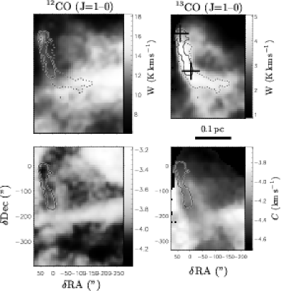
Figure 1: Maps of the Polaris (MCLD123+24.9) field in the ¹²CO(J=1–0) (left) and ¹³CO(J=1–0) (right) lines: (top) line integrated areas, (bottom) line centroid velocities. The offsets are in arcsec respectively to the (0,0) position: $l_{II}=123.68^{\circ}$, $b_{II}=24.93^{\circ}$. The two upper-left corners of the ¹²CO and ¹³CO maps coincide. The dashed contour level at 4$\,\mathrm{K\,km\,s^{-1}}$ in the $W_{\mbox{${}^{13}$CO}}$ map is meant to localize the region of largest column density and is reproduced in the $W_{\mbox{${}^{12}$CO}}$ map. The black contour is the 0.6 $\,\mathrm{K\,km\,s^{-1}}$–level of the CS(3-2) map (see Fig. 4) and is meant to localize the dense core in the rest of the paper. The two crosses show the positions of the HC₃N peaks (Heithausen et al. 2002). The linear scale is shown.

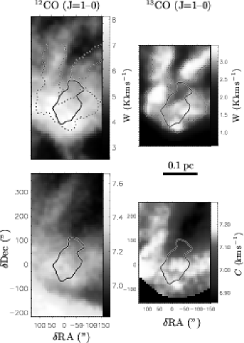
Figure 2: Same as Fig. 1 for the L1512 field observed at IRAM-30m. Offsets are in arcsec relative to the (0,0) position: RA(1950)= 05h00m54.5s, Dec(1950)=32^∘39’00”. The dashed contour level (3$\,\mathrm{K\,km\,s^{-1}}$ in the $W_{\mbox{${}^{13}$CO}}$ map) is reproduced in the $W_{\mbox{${}^{12}$CO}}$ map and helps localize the regions of largest column density. The dense core here (black contour) is identified with the 0.15$\,\mathrm{K\,km\,s^{-1}}$ contour of the HCO⁺(3-2) emission (see Fig. 4) and is reproduced in the rest of the figures. The linear scale is shown.

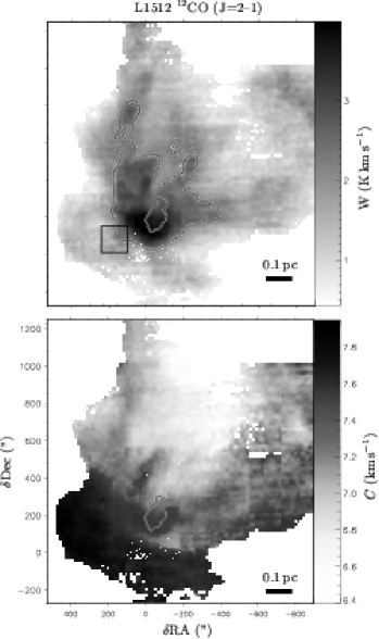
Figure 3: Maps of the ¹²CO(J=2–1) line integrated area $W$ (top) and line centroid velocities $C$ (bottom) of the L1512 field observed at the CSO. In both panels, a map of the same quantities computed with the high angular resolution data of the IRAM-30m is inserted in the CSO map at the relevant position. The dense core is identified as in Fig. 4 (black contour). The dashed contour corresponds to $W_{\mbox{${}^{12}$CO}}=2.5$$\,\mathrm{K\,km\,s^{-1}}$ and will be used in Fig. 11. The box is the location of the spectra map shown in Fig. 5. The (0,0) position of the CSO map is RA(1950)= 05h00m54.5s, Dec(1950)=32^∘36’00”. The linear scale is shown.

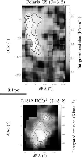
Figure 4: Map of integrated emission of the dense cores: IRAM-30m map of Polaris in the CS(3-2) line (top) and CSO map of L1512 in the HCO⁺(3-2) line (bottom).

In spite of their low average extinction, each field harbours a low mass dense core. The dense core in the Polaris field has been mapped in the CS(2-1), (3-2) and (5-4) lines (Heithausen 1999) and in a number of molecular species at a few positions only by Gerin et al. (1997). Recent observations of the dust thermal emission (Heithausen et al. 2002) show a clear peak of submillimeter dust continuum emission coinciding with the C¹⁸O peak of Falgarone et al. (1998). Well-defined and barely resolved peaks of HC₃N emission are found to be clearly displaced relative to the dust continuum maximum. They are indicated by two crosses in the ¹³CO map of Fig. 1. H₂ densities as large as a few 10⁵$\,\mathrm{cm^{-3}}$ in this dense core are derived from the multi-line analysis of Heithausen et al. (2002) and Gerin et al. (1997). Our unpublished map of CS(3-2) integrated emission is displayed in Fig. 4 and delineates the region of largest density. The contour level at 0.6 $\,\mathrm{K\,km\,s^{-1}}$of the CS(3-2) emission is shown in Fig. 1 to help localize the dense core. The ¹³CO(J=1–0) contour level of 4 $\,\mathrm{K\,km\,s^{-1}}$ is also drawn on Fig. 1 to indicate the region of column density larger than $\sim 4\times 10^{21}$$\,\mathrm{cm^{-2}}$.

In L1512, the dense core has been mapped in CS(2-1) by Fuller (1989) over several arc minutes. Lee et al. (2001) have mapped it over a more restricted area in the CS(2-1) and N₂H⁺ lines. A map of the HCO⁺(3-2) emission has been performed at the CSO in November 2002. The HCO⁺(3-2) line integrated emission is displayed in Fig. 4. As in other dense cores, the N₂H⁺ emission is more concentrated than the CS emission and the N₂H⁺ and HCO⁺(3-2) emissions have very similar boundaries. Again, in the following, we adopt the 0.15$\,\mathrm{K\,km\,s^{-1}}$ contour of the HCO⁺(3-2) emission as the boundary of the L1512 dense core. It is drawn in Figs. 2 and 3 to help locate the dense core. The maps of Figs. 1 to 3 confirm that dense cores, as traced by molecular lines such as CS, N₂H⁺ or HCO⁺ at millimeter wavelengths, are embedded in larger structures of moderate column density, traced by the ¹³CO lines, and further down in column density, by the ¹²CO lines. Note that the ¹²CO integrated emission in both fields is far from being isotropically distributed around the dense cores.

The analysis presented in the next sections has been conducted on the ¹²CO and ¹³CO data sets, when available. ¹²CO is the only available tracer of molecular gas down to H₂ column densities as low as a few 10²⁰$\,\mathrm{cm^{-2}}$. Reaching these limits is mandatory in order to be able to make a link with statistical works performed on HI data (e.g. Miville-Deschênes et al. (2003); Brunt (2003)), and to obtain large maps avoiding star forming regions. However, the large opacity of the ¹²CO line prevents the sampling of all the gas on the line of sight, most severely in regions close to the dense cores. The ¹³CO lines are thus used to analyze the gas in regions of intermediate column density between the transparent cloud edges traced by ¹²CO only and the dense cores. The areas available for statistical analysis in this line are smaller than those available in the ¹²CO line because of the different abundances of the two isotopomers. The two lines are therefore complementary.

4 Statistical analysis

4.1 Computation of line centroids and their increments

Figure 5: Representative spectra of the ¹²CO(J=2–1) CSO map, located in the box drawn in Fig. 3. On each spectrum, the window selected by the procedure designed to optimize the signal–to–noise ratio of the line integrated area is shown as thin vertical bars, as is the computed line centroid. The line temperature and velocity scales are given in the lower left corner.

Centroid velocities have been computed according to the algorithm described in Pety (1999). The line window used to compute the line centroid is critical (see Appendix A.1) and we have adjusted it locally to maximize the signal–to–noise ratio of the integrated area defined as SNR_a=$\Sigma_{1}^{m}T_{i}/\sqrt{m}\sigma$ where $T_{i}$ are the temperatures of the $m$ channels within the window and $\sigma$ the rms noise level of the spectrum. As the optimal window is expected to vary softly from one position to another, we smoothed the variations of the window edges with a median, moving boxcar filter of size $5\times 5$ pixels. The first moment is then computed on each spectrum using the optimal window found for its location. Fig. 5 illustrates the optimal windows found by this algorithm for a subset of the CSO map. This method also ensures that there is no significant emission out of the final optimal window. The line centroid increments are then computed over a lag $l$ expressed in pixels of the map. These increments are computed only between spectra that (i) have a SNR_a greater than 10.0 and (ii) have at least 4 neighbors with $\mbox{SNR${}_{a}$}\geq 10.0$. We show in Appendix A.2 how this threshold SNR_a = 10.0 ensures that our statistical analysis of velocity increments is not contaminated by thermal noise. For a given lag $l$, the increments are computed for half the possible orientations of the lag vector because if all the orientations are kept for each lag, each increment in the map appears twice with opposite signs. In the case of $l=3$ pixels, for instance, there are 16 different orientations, defined by the 16 neighbors of any position lying within the rings of radii 2.5 and 3.5 pixels. We kept only 9 different orientations for each position in the maps. Note that the smallest significant lag is $l=2$ pixels for the CSO map and $l=3$ pixels for the IRAM maps because the maps are oversampled.

4.2 Non-Gaussian wings in the centroid increment PDFs.

Table 3: Quantities used to normalize the $\delta C_{\mathrm{}}$–PDFs for each field and line and for the lag $l=3$ pixels: the offset applied to the increments to get a centered PDF (col. 3) and the standard deviation of the $\delta C_{\mathrm{}}$ values (col. 4). The ratio of these two quantities is given in col. 5.

Field	Line	$\langle\delta C_{\mathrm{3}}\rangle$	$\sigma_{\delta C_{\mathrm{3}}}$	${\langle\delta C_{\mathrm{3}}\rangle\over\sigma_{\delta C_{\mathrm{3}}}}$
		$\,\mathrm{km\,s^{-1}}$	$\,\mathrm{km\,s^{-1}}$
Polaris	12CO (J=1–0)	8.3 $\times 10^{-3}$	0.11	0.07
Polaris	13CO (J=1–0)	1.5 $\times 10^{-2}$	0.10	0.15
L1512	12CO (J=1–0)	1.2 $\times 10^{-2}$	0.05	0.24
L1512	13CO (J=1–0)	1.8 $\times 10^{-3}$	0.04	0.04
L1512	12CO (J=2–1)	1.3 $\times 10^{-2}$	0.09	0.015

Figure 6: PDFs of centroid velocity increments for increasing lag values $l$ given in arcsec and pixels within each frame. The PDFs have been computed from a) the ¹²CO (J=1–0) and b) ¹³CO (J=1–0) spectra maps of Polaris. The centroid increment scales have been normalized so that $\langle\delta C_{\mathrm{}}{}\rangle=0$ and $\sigma_{\delta C_{\mathrm{}}{}}=1$. The actual velocity dispersion of each distribution $\sigma_{\delta C_{\mathrm{}}(l)}$ is given in $\,\mathrm{km\,s^{-1}}$ in each frame. The dotted curves represent a Gaussian of zero mean and unit standard deviation.

Figure 7: Same as Fig. 6 for the L1512 field. The PDFs have been computed from the a) ¹²CO(J=1–0) and b) ¹³CO(J=1–0) IRAM-30m maps and c) ¹²CO (J=2–1) CSO map.

We have built the PDFs of the computed centroid increments for four different lags in each field and for each line. Hereafter, the PDFs of centroid increments will be called $\delta C_{\mathrm{}}$–PDFs or increment PDFs. They may also be seen as shear–PDFs since, as said in Section 2, the measured projection of the velocity is orthogonal to the plane in which displacements are measured (i.e. the plane of the sky).

Figs. 6 and 7 show the evolution of the $\delta C_{\mathrm{}}$–PDFs with increasing values of the lags for each map. The PDFs are normalized to zero mean and unit dispersion and a normalized Gaussian PDF with the same dispersion is shown, for comparison, as a dotted line. The quantities used for this normalisation are given in Table 3 for each map and a lag of 3 pixels. $\langle\delta C_{\mathrm{3}}\rangle$ is the offset applied to the increments at lag $l=3$ pixels to get a centered PDF and $\sigma_{\delta C_{\mathrm{3}}}$ is the standard deviation of the increments, for the same lag. The ratios ${\langle\delta C_{\mathrm{3}}\rangle\over\sigma_{\delta C_{\mathrm{3}}}}$ are given in Col. 5: they are all significantly smaller than unity. We therefore feel confident that the normalisation we apply does not affect the estimate of the $\delta C_{\mathrm{}}$–PDFs computed at small lags. The error bars drawn simply reflect the number of elements in each bin of the PDF. Note that the statistical significance of the largest increments is best for the CSO field because the number of independent spectra available in this map is about nine times larger than in the IRAM maps. This illustrates the importance of the size of the maps for this kind of statistical study where departures from Gaussianity are searched for and occur only with probabilities close to 10^-2 or below. In Appendix B, we compute the largest statistically significant lags for each map and two values of the numbers of bins in the PDFs, 30 and 8 bins. These numbers confirm that PDFs built with 30 bins, as in Figs. 6 and 7, are statistically significant up to lags of $\sim$ 6 pixels for the small fields and 12 pixels for the large one. They also show that the broad features in the PDFs, such as non-Gaussian wings, spreading over 4 bins or more, are significant up to lags of 12 pixels for all the fields.

All the sets of increment–PDFs exhibit non-Gaussian wings with departure from Gaussianity being more pronounced as the lag becomes small. The effect is the most visible in the large scale L1512 field, because the large number of independent spectra in that field reduces effects due to the poor sampling at large lags and makes the PDFs there the most symmetrical.

4.3 The influence of large–scale velocity gradients

Table 4: Influence of large scale velocity gradients. Difference between the observed extrema of line centroids in each map (col. 3), the associated scale $s$ (col. 4) and the corresponding observed large scale velocity gradients (col. 5), the contribution of this large scale gradient to a lag $l=3$ pixels (col. 6), the ratio of this contribution to the internal velocity dispersion at the same scale (col. 7), the exponent of the scaling of the standard deviation of the centroid increments with the lag at which they are computed (col. 8), the velocity gradients at scale $s$ inferred from this scaling and ascribed to turbulence (col. 9).

Field	Line	$\left|C_{\mathrm{min}}-C_{\mathrm{max}}\right|$	$s$	$\nabla v_{\mathrm{obs}}$	$\delta v_{3}$	${\delta v_{3}\over\sigma_{\delta C_{\mathrm{3}}}}$	$\zeta_{2}$	$\nabla v_{\mathrm{turb}}$
		$\,\mathrm{km\,s^{-1}}$	”/pc	$\,\mathrm{km\,s^{-1}}$ pc-1	$\,\mathrm{km\,s^{-1}}$			$\,\mathrm{km\,s^{-1}}$ pc-1
Polaris	12CO(1-0)	1.1	500/0.37	3.0	0.04	0.35	0.45	3.8
Polaris	13CO(1-0)	1.0	400/0.29	3.4	0.06	0.60	0.5	4.5
L1512	12CO(1-0)	1.2	600/0.44	2.7	0.05	1.0	0.62	2.7
L1512	13CO(1-0)	0.4	300/0.22	1.8	0.03	0.77	0.7	3.5
L1512	12CO(2-1)	1.4	1200/0.9	1.5	0.03	0.33	0.5	1.6

Figure 8: Scaling of the standard deviations of centroid increments with the lag $l$ used to compute the increments for the five fields and lines. Large symbols are used for the lags which give statistically meaningful results as explained in Appendix B. The exponents $\zeta_{2}$ listed in Table 4 have been determined for the range of lags which is statistically meaningful.

Large scale variations of the line centroid velocities are visible on Figs. 1 to 3. They most likely trace large scale velocity gradients. The observed values are derived from the two extreme values of the centroid velocity $C_{\mathrm{min}}$ and $C_{\mathrm{max}}$ and the size scale over which they are measured $s$ (Table 4). These numbers provide an estimate of the observed velocity gradients $\nabla v_{\mathrm{obs}}\approx\left|C_{\mathrm{max}}-C_{\mathrm{min}}\right|/s$ given in column 5 of Table 4. We note here that the values derived from two different lines in the same field are not necessarily the same because the lines do not quite sample the same gas, as discussed above. Unlike in other studies (Grosdidier et al. 2001; Miesch et al. 1999), we did not remove the contribution of large scale velocity gradients in our centroid increment computations. In this section, we explain why.

In the analysis of turbulence in HII regions, the large scale velocity gradients are related to the expansion of the warm ionized gas, driven by the pressure gradient of the HII region relative to the surrounding medium. It is thus justified to remove large scale gradients, prior to any statistical analysis of the turbulence within HII regions, as done by Grosdidier et al. (2001), because the HII region expansion is an ordered large scale motion and is not part of the inertial range of the turbulent cascade.

Miesch et al. (1999), who analyze the turbulence in molecular clouds, have different goals from ours. Their goal is to extract an homogeneous and isotropic subset of interstellar turbulence and compare it to laboratory experiments or direct numerical simulations. Instead, we search for regions of enhanced shear at small scales to localize bursts of dissipation. We show below that we are not limited in our analysis by large scale anisotropy. We first argue, following the results of numerical simulations of Burkert & Bodenheimer (2000) that turbulence itself with its steep power spectrum (i.e. most of the power is in the large scales) generates velocity gradients which may be interpreted as rotation at any scale. We show in Fig. 8 and Table 4 that this is indeed the case. The scaling of the standard deviation of the line centroid increments $\sigma_{\delta C_{\mathrm{}}{}_{l}}$ with lag $l$ is shown in Fig. 8. Up to lags of $\sim 100$ arc sec or about 12 pixels, $\sigma_{\delta C_{\mathrm{}}{}_{l}}\propto l^{\zeta_{2}}$. The values of $\zeta_{2}$ are given in Table 4. This scaling provides that of the turbulent velocity shear $\nabla v_{\mathrm{turb}}\propto l^{\zeta_{2}-1}$ with $l$. The turbulent velocity shear, $\nabla v_{\mathrm{turb}}$, inferred from this scaling law at the scale $s$ of the largest centroid differences is given in col. 9 of Table 4. Comparison of columns 5 and 9 shows that in all cases: $\nabla v_{\mathrm{obs}}\la\nabla v_{\mathrm{turb}}$. The large scale observed velocity gradients are therefore smaller than or comparable to those expected from the turbulent shear at the same scale, suggesting that they are part of the turbulent dynamics.

Last, we show that the large–scale gradients do not affect the small scale statistics which are of importance to the present analysis. The contribution of the large–scale gradients to the centroid velocity increments computed as $\delta v_{3}=\nabla v_{\mathrm{obs}}\times l$ for $l=3$ pixels are given in Table 4 for each map (col. 6). These values are then compared to the standard deviation of the $\delta C_{\mathrm{}}$–PDFs distribution (col. 7). In all cases, the ratio $\delta v_{3}/\sigma_{\delta C_{\mathrm{3}}}$ is smaller than or equal to unity. The contribution of the large–scale gradients to the centroid increments at small scale is therefore much smaller than the increments populating the non-Gaussian wings which extend up to 4 or 5 $\sigma_{\delta C_{\mathrm{}}}$ (see Figs. 6 and 7). Furthermore, the large scale gradient has a well-defined direction and therefore preferentially affects the increments computed along the same direction i.e. one increment out of 9 in the case of $l=3$ pixels (out of more for larger lags). The contribution of the large scale velocity gradient to increments computed over lags of different orientations is further reduced by the appropriate cosine. For these reasons, we are confident that keeping the large scale velocity gradients in the maps does not significantly distort the $\delta C_{\mathrm{}}$–PDFs of Figs. 6 and 7.

In summary, we did not remove large–scale velocity gradients prior to our statistical analysis for two reasons: (1) there is evidence for the large–scale gradients to be part of the turbulent dynamics we analyze and (2) their value is such that their contamination of the small scale statistics on which we focus here, is negligible.

5 Spatial distribution of the non-Gaussian centroid increments: a new kind of small scale structure

5.1 The positions populating the non-Gaussian wings of the increments PDFs are not randomly distributed: they form elongated structures

Table 5: Characteristics of the maps of averaged centroid increments for each field and line: thresholds used to define the subsets of positions populating the non-Gaussian wings of $\delta C_{\mathrm{}}$–PDFs (col. 3), peak increment (col. 4) and background (col. 5) values, square of the contrast of the peak to background value (col. 6), average of the line profile velocity dispersion over the field (col. 7), surface filling factor of regions where $\left|\delta C_{\mathrm{}}\right|{}>\left|\delta C_{\mathrm{0}}\right|$ (col. 8) and fraction of dissipation in these regions (col. 9, see Section 7). The last column is the average linewidth in each field (see Section 6.3).

Field	Line	$\left|\delta C_{\mathrm{0}}\right|$	$\left|\delta C_{\mathrm{max}}\right|$	$\left|\delta C_{\mathrm{bg}}\right|$	$(\delta C_{\mathrm{max}}/\delta C_{\mathrm{bg}})^{2}$	$\langle\sigma_{u}\rangle$	$f_{s}$	$f_{\epsilon}$	$\langle\Delta v\rangle$
		$\,\mathrm{km\,s^{-1}}$	$\,\mathrm{km\,s^{-1}}$	$\,\mathrm{km\,s^{-1}}$		$\,\mathrm{km\,s^{-1}}$			$\,\mathrm{km\,s^{-1}}$
Polaris	12CO (J=1–0)	0.1	0.4	0.06	39	0.8	0.29	0.65	0.8
Polaris	13CO (J=1–0)	0.1	0.4	0.05	82	0.4	0.20	0.62	0.38
L1512	12CO (J=1–0)	0.05	0.1	0.03	15	0.3	0.29	0.61	0.30
L1512	13CO (J=1–0)	0.03	0.08	0.02	17	0.2	0.39	0.74	0.17
L1512	12CO (J=2–1)	0.09	0.4	0.06	45	0.3	0.18	0.53	0.29

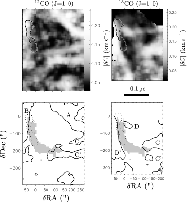
Figure 9: Top panels: Maps of the averaged centroid increments $\left|\delta C_{\mathrm{}}\right|$ in Polaris computed with a lag of 3 pixels from the ¹²CO(J=1–0) lines (left) and the ¹³CO(J=1–0) lines (right). The solid contour localizes the dense core (see Fig. 1). The bottom panels are sketches meant to emphasize the relative orientation of the region of large column density traced by ¹³CO (grey area), the dense core (dashed contour) and regions of large centroid increments where $\left|\delta C_{\mathrm{}}\right|$ $>$ $\left|\delta C_{\mathrm{0}}\right|$ (black contours). The thresholds $\left|\delta C_{\mathrm{0}}\right|$ are those listed in Table 5. The letters are the labels used in the text.

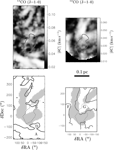
Figure 10: Same as Fig. 9 for the L1512 field observed at IRAM.

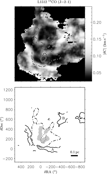
Figure 11: Same as Fig. 9 for the large scale L1512 field. The dot-dashed contour is the same as in Fig. 3.

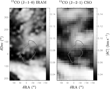
Figure 12: Maps of average centroid increments of the same region of the L1512 field computed from the IRAM-30m ¹²CO(J=1–0) map (left) and the CSO ¹²CO(J=2–1) map (right). Note the remarkable quantitative agreement between the two maps.

We have seen in the previous section that, in most cases, the departure of the increment PDFs from a Gaussian distribution is as large as the lag is small. We are here interested in tracing the locations of the positions for which the small scale increment values build up the non-Gaussian wings. We display in Figs. 9 through 11 the spatial distribution of the increments computed for lags of three pixels. The lag value $l=3$ pixels is the smallest significant lag in the IRAM maps because the maps are Nyquist sampled or better: adjacent pixels are therefore not independent (see Table 1).

The spatial distributions of the centroid increments are shown as azimuthal averages over the 16 possible directions because it allows a more compact presentation of the results. In the rest of the paper, we note $\left|\delta C_{\mathrm{}}\right|$ the azimuthal average of the modulus of all the oriented centroid increments computed at a given position, for lags of three pixels. The thresholds, $\left|\delta C_{\mathrm{0}}\right|$, given in Table 5, has been chosen to isolate the regions where more than half of the oriented increments belong to the non-Gaussian wings of the $\delta C_{\mathrm{}}$–PDFs. These thresholds are close to the standard deviations $\sigma_{\delta C_{\mathrm{3}}}$ of the increment–PDFs for $l=3$ pixels. Note that the averaging produces increment values smaller by factors up to a few than the original values used to build the PDFs. This effect is illustrated in the cuts of Figs. 13–16 where the variations of the centroid and of the centroid increments before and after azimuthal averaging are shown as a function of position.

In Figs. 9–11, the uniform black areas correspond to positions where increments are not computed because at least one of two spectra used either has a SNR_a value below 10.0 or is too isolated (i.e. with less that 4 contiguous neighbors with $\mbox{SNR${}_{a}$}>10.0$). The black contours drawn after the CS(3-2) or HCO⁺(3-2) maps help locate the dense cores.

In the sketches of Figs. 9–11, the black contours labelled by letters follow the thresholds $\left|\delta C_{\mathrm{0}}\right|$. These contours are therefore intended to trace the structures delineated by the positions where the original, non averaged, increments are larger than a few $\sigma_{\delta C_{\mathrm{3}}}$ and belong to the non-Gaussian wings of the $\delta C_{\mathrm{}}$–PDFs.

Two characteristics of these structures may be derived from Figs. 9–11. Firstly, the spatial distribution of the largest averaged increments is not random. They are concentrated in specific regions and appear to form elongated structures, almost straight in several cases, and covering only a small fraction of the maps. Secondly, the $\left|\delta C_{\mathrm{}}\right|$ values in these structures are well above the background fluctuations of the increments in the maps. Table 5 gives the background values $\left|\delta C_{\mathrm{bg}}\right|$ computed as the median of all the values smaller than the thresholds $\left|\delta C_{\mathrm{0}}\right|$ and the largest values of increments $\left|\delta C_{\mathrm{max}}\right|$ in the maps. It shows that the largest values are between 4 and 9 times above the background values, far above statistical fluctuations.

Last, it is remarkable that similar spatial distributions are found for the large increments computed in the same field with two independent data sets i.e. from two different telescopes and two different lines, ¹²CO (J=1–0) and (J=2–1). Fig. 12 allows a comparison of the patterns found for the centroid increments in the L1512 field from the IRAM-30m and CSO maps. The morphological and quantitative agreement between the two maps fully supports the reality of these structures. In Section 6, we discuss why they do trace the shear of the velocity field.

The smallest lags of three pixels introduce an effective resolution, ascribing a size of three pixels to unresolved variations of the line centroid. But some of the structures traced by the largest increments are resolved by the observations. This last characteristic is also seen in the cuts of Figs. 13–16. In the RA cut across the L1512 field, the peak of increment visible at RA offset $\sim 200"$ is due to the steepening of the variation of the line centroid over 6 consecutive pixels, from offset $\sim 300"$ to 200” or more than three CSO beamwidths. The half-power width of this feature (above the background value), $\sim 0.05$ pc, is therefore resolved by the procedure of computing increments over lags of 3 pixels. We illustrate with the other cuts that several of these structures are actually resolved, with thicknesses of the order of 0.05 pc, up to 0.08 pc.

Figure 13: Cuts in the ¹²CO line of the Polaris field in RA, averaged over the indicated Dec range. The histograms are the cuts of increment centroids: raw values in the top panel, averaged in azimuth as explained in Section 5.1 in the bottom panel. The other cuts are the centroid velocities (top) and integrated area (bottom). The letters correspond to those of Fig. 9.

Figure 14: Same as Fig. 13 for the ¹³CO line of the Polaris field. Here the cuts are in RA, averaged over the indicated Dec range.

Figure 15: Same as Fig. 13 for the large scale L1512 field. The letters correspond to those of Fig. 11.

Figure 16: Same as Fig. 14 for the large scale L1512 field.

5.2 Comparison with the results of Miesch et al. (1999)

The non-random distribution of the largest centroid velocity increments seems at odd with the spotty distribution found by Miesch et al. (1999) in their maps of centroid velocity differences of several star forming regions. However, we consider that our results agree with theirs for the following reason. Their method, as explained in Section 4.3, is different from ours because they first remove a smoothed value from the line centroid values in their maps. The centroid velocity fluctuations they obtain with this procedure are already of the same nature as a velocity increment, as shown by Lis et al. (1996). It is therefore meaningful to compare their maps of centroid fluctuations with our maps of centroid increments. Their maps of centroid velocity fluctuations (their Figs. 4 and 5) do indeed exhibit spatial structures. The largest values appear in several cases to form narrow and elongated structures similar to those we find. The spotty distribution is found only once they compute the increments of these former maps of velocity fluctuations. What they call centroid velocity differences cannot be compared to what we compute.

A more detailed comparison of the two sets of results would not be meaningful for several reasons. The signal-to-noise ratios of our data given in Table 2 are significantly better than those of Miesch et al. (1999). Their SNR values range between 4.5 and 8.9, except for HH83, which has SNR=19.7 but is their smallest field. The nature of the fields is also different. While we analyze only quiescent fields in the present paper, Miesch et al. have analyzed active star forming regions where many shocks, driven by the young stars, interact and probably generate considerable small scale structure in the patterns of the vorticity. Last, most of the fields being at distances larger that the nearby fields studied here, the angular characteristic scales of the structures (if any) are expected to be smaller.

5.3 The regions of largest centroid increments are not coinciding with density nor column density peaks

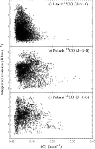
Figure 17: Scatter plots of the integrated emission versus the centroid increments for three data sets analyzed.

The sketches of Figs. 9 to 11 allow a comparison of the structures of largest increments with the concentrations of matter, whether they are large column density or large density structures or both. The dotted contours delineate the dense cores and the grey areas those where the ¹³CO(J=1–0) integrated emission is larger than 3 and 4 $\,\mathrm{K\,km\,s^{-1}}$, for L1512 and Polaris respectively, which corresponds to $N(\mbox{H${}_{2}$})>$ a few $10^{21}$$\,\mathrm{cm^{-2}}$, about 10 times the average column density of the large scale environment. The main result visible in those figures is that none of the regions of largest increments coincides, even in projection, with either a dense core (i.e. a density peak) or a column density peak.

This result is better seen in the cuts of Figs. 13–16: the large variations at small scale of the line centroid, at the origin of the large increment values, do not coincide with column density extrema. Such a coincidence would be expected if the line centroid variations were due to the overlap on the line of sight of unrelated gas components. In that case, an extremum of column density would coincide with the region of large centroid increment, which is that over which the two components are intercepted, producing a modified (locally broader) line profile. This lack of correlation is also seen in the scatter plots of Fig. 17 where the largest increments are in no case associated with extrema of column density. Conversely, the largest increments tend to occur at the positions were the integrated areas are the smallest.

5.4 Link between the orientation of these structures and that of density structures

The previous section shows that the structures traced by the regions of largest centroid increments at small scale do not coincide (in projection) with the dense cores nor the column density extrema in the maps.

Nonetheless, this statement does not mean that these small scale structures are unrelated to the dense cores. The orientation of the most elongated structures tend to be related with that of the dense cores. In the Polaris field, the structure labelled C’ in the ¹²CO map, appears as a prolongation of the bright ¹³CO structure, which seems to be an extension of the dense core itself (see sketches of Fig. 9). The structures B and D’ are adjacent and parallel to the edge of the dense core, as is seen also in the cuts of Fig. 14. In the L1512 field (Fig. 11), similar patterns are visible. The two southern structures A and A’ frame in projection the region of bright ¹²CO lines (dot-dashed contour), and the structure B is elongated in the same direction as that of the filament of matter seen in ¹³CO and ¹²CO and the orientation of the dense core itself as mapped in HCO⁺. Since the velocity is continuous between the structures of large increments and those of matter (see maps of line centroids in Figs. 1–3), it is most likely that they are connected in the 3–dimensional space.

5.5 Volume filling factor of the largest increment structures

For each field, in addition to the maximum value of the increments in the map, $\left|\delta C_{\mathrm{max}}\right|$ and the background value $\left|\delta C_{\mathrm{bg}}\right|$ defined in Section 5.1, Table 5 also gathers the fraction $f_{s}$ of pixels in the map where the centroid increments are larger than the thresholds $\left|\delta C_{\mathrm{0}}\right|$. $f_{s}$ may be understood as their surface filling factor in the maps. From its values, one derives volume filling factors of the regions of largest increments of at most a few %. Assuming that the depth of the structures along the line of sight is comparable to their projected thickness, $d$, and that the extent of the cloud along the line of sight, $L$, is provided by the large scale maps (Falgarone et al. 1998), $f_{v}\sim f_{s}d/L$. For $d\sim 0.05$ pc and $L\sim 1$ pc, $f_{v}\sim$ a few % or less.

6 Discussion

The subset of spectra shown in Fig. 5 encompasses one of the regions where the centroid increments are the largest. Fig. 5 shows that the optimal window found to compute the line centroids varies only by very small amounts from one spectrum to the next. This illustrates that the measured centroid increments are due to small variations in the shapes of the line profiles from one line of sight to the next. These variations may have several origins, unrelated to the structure of the velocity field: optical depth effects, gas temperature or density fluctuations. We show in the following section that our interpretation of these variations as tracers of small scale velocity shears is justified.

6.1 Optical depth effects

The optical depth of the lines used introduces a possible bias in the sampling of the velocity field performed by the spectra. Indeed, optically thick lines tend to sample preferentially foreground material.

However, the maps of centroid increments built from the ¹³CO and ¹²CO lines, although not exactly the same, are reminiscent of each other, suggesting that the two lines sample about the same gas (see Figs 9–10). This is also suggested by the similarity of the maps obtained in L1512 with two different ¹²CO transitions of different optical depths (Fig. 12). These results support the concept of low effective optical depth of the ¹²CO lines discussed in Martin et al. (1984). Falgarone et al. (1998) also inferred a low effective optical depth in the ¹²CO lines of the fields analyzed here (except in the projected area of the dense cores), on the basis of the uniformity of the excitation temperature. Note that a low effective optical depth of the ¹²CO lines is to be expected in these fields (as opposed to brighter molecular clouds) because a large velocity dispersion of the gas, leading to a large escape probability of the photons in velocity space, is combined with low gas column densities. The same similarity is found between maps of centroid increments built from the ¹³CO and C¹⁸O spectra of the environment of the L1689B dense core (Pety et al. in preparation), suggesting that optical depth effects are not seriously affecting the centroid increment determinations.

This result illustrates a major strength of the line centroid analysis. On the one hand, centroids are velocity moments and as such provide more weight to velocities far from the line centroids, i.e. the line wings. The wings are the parts of the line profiles the least affected by optical depth effects. On the other hand, our method which limits the range of velocities used to compute the centroid (see Section 4.1), limits the noise contribution, particularly in the line wings. We thus argue that there is a velocity range in spectrally well-sampled line profiles, neither too far in the line wings (to avoid noise artefacts) nor too close to the line centroid (to avoid optical depth artefacts), which carries enough information on the velocity field to be used on statistical grounds.

Last, self-absorption is also unlikely in those low brightness core environments because the excitation temperature of the ¹²CO and ¹³CO lines is remarkably uniform as was shown by the scatter plots of the (J=1–0) to (J=2–1) ¹²CO and ¹³CO lines (Falgarone et al. 1998). For self-absorption to occur the optical depth must exceed unity and the foreground material must have a lower excitation temperature.

6.2 Role of temperature fluctuations

It might be argued that the variations of line centroids traced by the ¹²CO lines are due only to variations of the gas kinetic temperature. This might be the case in bright sources where the ¹²CO lines are thermalized. But it has to be appreciated that in the fields under study here the ¹²CO lines are weak (less than 5 K) while the gas is poorly shielded from the ambient UV field (H₂ column densities less than a few $10^{21}$$\,\mathrm{cm^{-2}}$) and thus likely to be much warmer than 5K. It means that either the lines are subthermally excited, in which case their excitation is mostly radiative, or that they are thermally excited in small structures with a large beam dilution factor. In either case, the line profile variations are not determined by variations of the gas kinetic temperature but by those of the radiative excitation and/or beam filling factor, which both depend on the velocity field (Falgarone et al. 1998).

6.3 Role of density fluctuations unrelated to the velocity field

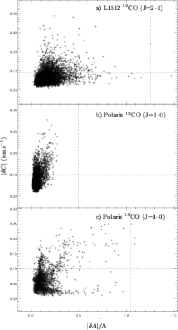
Figure 18: Scatter plots of the azimuthally averaged increments, $\left|\delta C_{\mathrm{}}\right|$, versus the relative variations of the line integrated area, $\left|\delta A\right|$/A, for three data sets. The horizontal lines show the $\left|\delta C_{\mathrm{0}}\right|$ thresholds separating the Gaussian kernel from the non-Gaussian wings in the $\delta C_{\mathrm{}}$-PDFs. The vertical lines are an estimation of the required column density relative variations to produce centroid increments of the order of $\left|\delta C_{\mathrm{max}}\right|$ in each field.

In this section, we discuss the influence of column density or density variations, independent of the velocity field, on the velocity increments that we measure. Under the optically thin hypothesis, $dN(u)\propto T(u)\,du$ where $dN(u)$ is the column density of gas at the projected velocity $u$ within $du$. The centroid velocity defined in Eq. (1) is therefore also

$$C_{\mathrm{}}=\frac{\int u\,dN(u)}{\overline{N}}\quad\mbox{with}\quad\overline{N}=\int dN(u).$$ (3)

The centroid increment between lines of sight 1 and 2 can thus be written

$$\delta C_{\mathrm{1-2}}=\displaystyle\left[\frac{\int u_{1}dN_{1}(u_{1})}{\overline{N}_{1}}\right]-\displaystyle\left[\frac{\int u_{2}dN_{2}(u_{2})}{\overline{N}_{2}}\right].$$ (4)

From this expression, it is obvious that $\delta C_{\mathrm{1-2}}=0$ if the two lines of sight differ only by their total column density, the velocity structure being the same i.e. $N_{2}(u_{2})\propto N_{1}(u_{1})$ for all velocities. In this case the two integrated line profiles are simply homothetic.

Let us consider another simple case in which the total column density $N$ along the two lines of sight is approximately the same, the only difference being that a fraction of the gas at projected velocity $u_{1}$ on the first line of sight is at $u_{2}$ on the other. This is possible, for instance, in the perspective of matter distributed in a large number of very small structures, possibly virialized in the potential well of the cloud. Then $\delta C_{\mathrm{1-2}}=(u_{1}-u_{2})\,\delta N/N$ where $\delta N$ is the column density of the gas which is at different projected velocities on each line of sight. We estimate below the value of $\delta N/N$ required to produce centroid increments of the order of $\left|\delta C_{\mathrm{max}}\right|$ in each field. We assume that the velocity difference $u_{1}-u_{2}$ is of the order of magnitude of the average linewidth in each field $\langle\Delta v\rangle$ given in Table 5, $u_{1}-u_{2}\sim\langle\Delta v\rangle$. Therefore an estimate of the required column density fluctuations is: $\delta N/N\sim\left|\delta C_{\mathrm{max}}\right|/\langle\Delta v\rangle$. The latter ratio can be computed from the values in Table 5 and is equal to 1.25, 0.5 and 1.05 for the three fields of Fig. 18, respectively. Now, if we assume that the relative variations of the line integrated areas trace those of gas column density, we can check how the observed fluctuations of column density compare with the above values. This may be seen in the scatter plots of the averaged increments versus the relative variations of the line integrated area, $\left|\delta A\right|/A$ (Fig. 18). These scatter plots are shown only for the three maps where the statistics are the least affected by the dense core. The values of $\left|\delta C_{\mathrm{max}}\right|/\langle\Delta v\rangle$ and of the threshold $\left|\delta C_{0}\right|$ are indicated for each field. The scatter plots show that, except for a few lines of sight of the Polaris ¹³CO map, the observed relative variations of column density (or $\left|\delta A\right|/A$) at the positions of increments populating the non-Gaussian wings (i.e. increments above the thresholds $\left|\delta C_{\mathrm{0}}\right|$) are smaller than the minimum value estimated above. In the large scale L1512 field and the Polaris field as seen in ¹²CO, it is therefore unlikely that the observed centroid increments trace small scale column density fluctuations due for instance to randomly distributed clumps. This is also supported by the fact that the structures traced by the large centroid increments form spatially coherent patterns and are not randomly distributed as would be expected for randomly moving clumps. We thus conclude that the contribution of small scale random column density variations to the observed centroid increments is not dominant.

These small scale column density fluctuations could trace density fluctuations. They occur over lags of 3 pixels or $l\sim 5000$ AU (see Table 1). The corresponding density enhancements are therefore expected to occur over the same small scale $l$. Thus, $\delta n/n\sim(\left|\delta A\right|/A)\,(L/l)$ where $L$ is the depth of the cloud. For $\left|\delta A\right|/A=0.5$ and $L=1$ pc, $\delta n/n=25$. These might be supersonic shocks with Mach numbers of about 5, in which case the density and velocity fields are closely correlated. However, such large density enhancements would produce variations of the CO(J=2–1)/CO(J=1–0) line ratio in the weak regions of the fields, variations which are not observed (Falgarone et al. 1998).

The tenuous variations of the line profiles at the origin of the large centroid increments at small scale are therefore most likely ascribed to large velocity shears at small scale.

7 Possible link with the dissipation of turbulence

Our statistical analysis of the environment of two low mass dense cores leads to two main results: (i) the PDFs of line centroid increments (or velocity shears) have non-Gaussian wings as more pronounced as the lag over which they are computed is small, and (ii) the spatial distribution of the largest shears is not random and reveals often resolved and elongated structures not coinciding with density nor column density peaks. These are predominantly velocity structures.

The first property is a characteristic shared by incompressible turbulence, compressible turbulence and compressible, magnetized turbulence and is a signature of the intermittency of the velocity or current density fields. Our results therefore suggest that the observed distributions of large shears may trace regions of intense vorticity reminiscent of those responsible for the intermittency of turbulence. Note that these regions of intense vorticity are embedded in the bulk of the flow and that the large centroid increments are only tracers of their presence in the flow. In other words, a small scale structure of large vorticity, embedded in the bulk of the flow, can be at the origin of a small variation of the line centroids, along the boundary of two large scale regions of more uniform centroid velocity, i.e. the large eddies.

We have argued that the large shears are unlikely to trace shocks but we cannot rule out the fact that the vorticity extrema are fossil structures of shocks, already disrupted.

If the largest shears that we have detected trace local enhancements of the vorticity and therefore dissipation, as discussed in the Introduction, an estimate of the local enhancement of the dissipation rate in those regions is provided by the ratio $(\delta C_{\mathrm{max}}/\delta C_{\mathrm{bg}})^{2}$ (Table 5) because the dissipation rate follows the square of the vorticity (or of the velocity shear) (Landau & Lifshitz, 1987). The local enhancements are large, between 15 and 80 (Table 5). It is interesting to note that the smallest values of $(\delta C_{\mathrm{max}}/\delta C_{\mathrm{bg}})^{2}$ are obtained in the close vicinity of the L1512 dense core (IRAM field) and the largest in Polaris and in the large scale environment of L1512 (CSO field). This may reflect the fact that turbulent dissipation is a less violent process within a dense core which is already formed. We also note that even the weakest structures in the maps of $\left|\delta C_{\mathrm{}}\right|$ have a contrast larger than 2 above the background and therefore correspond to a dissipation rate locally 4 times larger than in the bulk of the field (see for instance the weak structures, labelled B and C, in the North of the IRAM L1512 ¹²CO map).

Last, the quantity $f_{\epsilon}=\sum_{\left|\delta C_{\mathrm{}}\right|{}>\left|\delta C_{\mathrm{0}}\right|}\left|\delta C_{\mathrm{}}\right|{}^{2}/\sum_{\mathrm{all}}\left|\delta C_{\mathrm{}}\right|{}^{2}$ (Table 5) may be understood as the fraction of the dissipation taking place in the regions of large increments (those populating the non-Gaussian wings). The underlying assumption is that the ratio of the actual dissipation rate to $\left|\delta C_{\mathrm{}}\right|{}^{2}$ is the same in the regions where the increments populate the Gaussian cores of the PDFs (the bulk of the fields) as in those populating the non-Gaussian wings. Under this assumption, the values of Table 5 show that a significant fraction (more than half) of the total dissipation takes place in the ensemble of small scale structures filling a volume close to a few % of the cloud volume, as estimated above.

8 Conclusion

We have found a new kind of small scale structure in the environment of low mass starless dense cores.

They emerge in the maps of line centroid increments between adjacent spectra as regions between 4 and 9 times brighter than the background fluctuations. They are essentially velocity structures because they are not coinciding with any detected sufficient increase in the column density or density. They are small scale, often elongated, structures. A few are resolved by the observations with thicknesses up to 0.08 pc. Most of them are not resolved i.e. smaller than 0.02 pc, the effective resolution due to the smallest lag available to compute the increments.

The measured projected velocity being orthogonal to the plane of the sky, in which lags are measured, the centroid velocity increments trace one component of the shear of the velocity field. The shear-PDFs exhibit non-Gaussian wings which are the most prominent for the smallest lag. For this reason, we ascribe these structures to turbulence by analogy with the behavior of such PDFs in laboratory flows or numerical simulations of compressible turbulence. The new structures delineate the locus of positions where the increments are the largest and populate the non-Gaussian wings.

These structures therefore possibly trace regions of enhanced dissipation of turbulence in the observed fields. The nature of the dissipation process is not determined by the observations: it could be either viscous dissipation, ion-neutral collisions or enhanced current densities. These structures are unlikely to trace shocks, but they may trace the remanent vorticity generated by shocks already disrupted. In this picture, a significant fraction of the turbulent energy present in the field would be dissipating in those structures filling less than a few % of the cloud volume.

Last, the structures display some connexion with the tracers of dense gas, such as shared orientations and velocity and space pattern continuity. Before we can make a link between such structures and the formation of dense cores, we need to investigate control fields i.e. molecular clouds without dense cores (Hily-Blant et al. in preparation) and with moderate star formation activity (Pety et al., in preparation).

Appendix A Role of the thermal noise in the statistical analysis

Thermal noise in the spectra affects the estimation of the line centroid velocity. It thus could be that thermal noise largely contributes to the non-Gaussian wings of the $\delta C_{\mathrm{}}$–PDFs. This influence of thermal noise is relatively more important at small lags where the increments are the smallest because of the scaling laws of turbulence. In section A.1, we show that most of the large increment values are significantly above the thermal noise contribution. And in section A.2, we present results of numerical simulations performed to answer two questions: (i) can thermal noise create non-Gaussian wings on intrinsically (originally) Gaussian $\delta C_{\mathrm{}}$–PDFs and (ii) how does thermal noise affect the shape of an $\delta C_{\mathrm{}}$–PDF which has intrinsic non-Gaussian wings?

A.1 Increment SNR

The uncertainty on the centroid velocity of a spectrum scales as (Pety 1999):

$$\Delta C_{\mathrm{}}\propto W_{\mbox{}}/\mbox{SNR${}_{a}$}$$ (5)

where $W_{\mbox{}}$ is the width of the optimal window (see Section 4.1). The uncertainty on the centroid velocity increments, $\Delta(\delta C_{\mathrm{}}{})$, can be approximated as the quadratic sum of the uncertainties on the centroid of each spectrum in the pair. Fig. 19 shows the scatter plots of the centroid velocity increments signal–to–noise ratios (SNR${}_{\delta C_{\mathrm{}}{}}$, defined as the ratio of $\delta C_{\mathrm{}}$ to its uncertainty) versus the centroid velocity increments for the five maps. Here all the directions of the pairs are considered.

The butterfly shape of these scatter plots is due to the fact that the centroid uncertainties are bounded, essentially by the two extreme values of SNR_a, since $W_{\mbox{}}$ does not vary much in a map. We impose the lowest SNR_a value to be 10.0 (see Appendix A.2). The upper value reflects the finite noise level and the peak line intensity in each map. The $\delta C_{\mathrm{}}$–uncertainties, $\Delta(\delta C_{\mathrm{}}{})$, defined as above, are therefore also bounded. We call these boundaries $A$ and $B$ so that $1/A\leq\Delta(\delta C_{\mathrm{}})\leq 1/B$. We then obtain

$$B*\left|\delta C_{\mathrm{}}\right|{}\leq\mbox{SNR${}_{\delta C_{\mathrm{}}{}}$}\equiv\left|\frac{\delta C_{\mathrm{}}{}}{\Delta(\delta C_{\mathrm{}}{})}\right|\leq A*\left|\delta C_{\mathrm{}}\right|{}.$$ (6)

The $A$ and $B$ boundaries thus appear as the slopes of the lines that limit the scatter plots of Fig. 19.

These scatter plots also show that the structures delineated by the largest centroid increments and shown in Figs. 9 to 11 have large SNRs. Clearly these structures are far above the noise level, as was already suggested by the good agreement between the IRAM and CSO results for the L1512 core (see Fig. 12 and section 5.1).

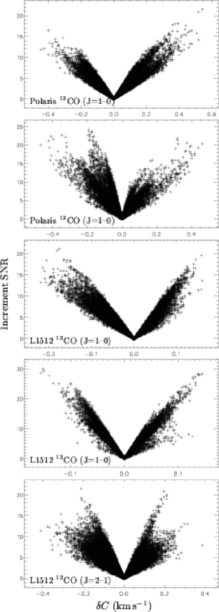
Figure 19: Scatter plots of the $\delta C_{\mathrm{}}$ signal–to-noise ratio (defined as the ratio of $\delta C_{\mathrm{}}$ to its uncertainty) versus the $\delta C_{\mathrm{}}$-values for the five data sets analyzed. These scatter plots show that the structures delineated by the largest centroid increments and shown in Figs. 9 to 11 have large SNRs.

A.2 Simulations

Figure 20: Results of numerical simulations showing the evolution of the shape of the normalized $\delta C_{\mathrm{}}$–PDFs as thermal noise is progressively added to maps of noiseless Gaussian line profiles. The two maps have the same spatial distribution of line areas and widths as the real data of the L1512 large scale field. Their difference lies in the distribution of line centroids: it is Gaussian (top panels) or identical to the real data (bottom panels) (see text). Two different SNR_a thresholds (i.e. 3 and 10) are used in the computation of the centroid velocity increments. For the Gaussian velocity field, thermal noise can create non-Gaussian wings to the $\delta C_{\mathrm{}}$–PDFs, only when the SNR_a threshold is 3 and for the largest noise. In comparison, the evolution in the bottom panels shows that the L1512 velocity field has intrinsic non-Gaussian statistical properties. The Gaussian PDF in the case of largest noise and SNR_a is due to poor sampling (see text).

Figure 21: Evolution of the number of spectra whose SNR_a value is above a given threshold (3 for the dotted line and 10 for the plain line) as a function of the noise level.

We computed two spectra maps made of Gaussian lines with the same line areas and widths at each position as in the L1512 large scale field. The first one also has the same spatial distribution of centroid velocities as the L1512 field. For the second one, the spatial distribution of centroid velocities has been computed from a random, Gaussian data cube whose power spectrum is a power law of -5/3 exponent. It has been checked that this cube does not show intermittent behavior, i.e. $\delta C_{\mathrm{}}$–PDF are Gaussian at all scales (Pety 1999). These two spectra maps are respectively referred to as the L1512 velocity field and the Gaussian velocity field.

To mimic thermal noise, we added random numbers sampled from a Gaussian law of zero mean and a given standard deviation, to the intensities of all channels. We checked that the average noise of the spectra in the map is the value of this standard deviation. The original L1512 CSO field has quite a uniform noise distribution of average value 0.2$\,\mathrm{K}$. We thus fixed the standard deviation of Gaussian noise to values between 0.02 and 0.8$\,\mathrm{K}$ to explore a fair range of SNR_a (the spectra area being kept fixed). We then used our algorithm to compute the centroid map from the spectra map (see section 4.1). We used two different SNR_a thresholds (i.e. 3 and 10) to thoroughly explore thermal noise effects. All the $\delta C_{\mathrm{}}$–PDFs have been computed for a lag of 3 pixels, and normalized to zero mean and unit dispersion.

Fig. 20 shows normalized $\delta C_{\mathrm{}}$–PDFs for 3 different values of noise levels: 0.002$\,\mathrm{K}$ equivalent to the noise–free case, 0.2$\,\mathrm{K}$ equal to the value of the real L1512 data and 0.8$\,\mathrm{K}$, the largest value. For the Gaussian velocity field, thermal noise can create non-Gaussian wings to the $\delta C_{\mathrm{}}$–PDFs. However, those non-Gaussian wings appear only when the SNR_a threshold is 3 and for the largest noise values. This implies that thermal noise cannot be responsible for the non-Gaussian wings seen in the $\delta C_{\mathrm{}}$–PDFs computed on the real L1512 data: the L1512 velocity field has intrinsic non-Gaussian statistical properties.

For the L1512 Velocity Field (see Fig. 20), thermal noise does not change the normalized $\delta C_{\mathrm{}}$–PDF shape for typical noise values (i.e. 0.2$\,\mathrm{K}$). $\delta C_{\mathrm{}}$–PDF shapes change only for the highest noise values. In particular, the $\delta C_{\mathrm{}}$–PDF can become Gaussian when the SNR_a threshold is 10. This is just a sampling effect. Indeed, Fig. 21 shows the number of points in the spectra map whose SNR_a values are above the threshold, as a function of the map noise level. It can be seen that the number of spectra with $\mbox{SNR${}_{a}$}\geq 10.0$ (solid line) decreases much faster than the number of spectra with $\mbox{SNR${}_{a}$}\geq 3.0$ (dotted line). Due to the anticorrelation between high area and high $\left|\delta C_{\mathrm{}}\right|$ regions (see Fig. 17.a), the remaining points naturally have a velocity field with a Gaussian statistic.

Appendix B Sampling effects

Table 6: Largest significant lags for the $\delta C_{\mathrm{}}$–PDFs in each field. The field sizes are $N$ and $M$ in pixels and the largest significant lags are given (in pixels) for $\delta C_{\mathrm{}}$–PDFs built with 8 (col. 6) and 30 (col. 7) bins.

Source	Line	$N$	$M$	$l_{\mathrm{max}}(8)$	$l_{\mathrm{max}}(30)$
Polaris	12CO (J=1–0)	48	64	12	6
Polaris	13CO (J=1–0)	40	56	12	6
L1512	12CO (J=1–0)	40	80	13	7
L1512	13CO (J=1–0)	56	40	12	6
L1512	12CO (J=2–1)	90	96	21	11

Statistical estimators are significant only if they are measured over a large enough number of realizations. The number of realizations of the increments at a given lag, increases as the lag decreases. We compute below the largest statistically significant lag in each available map. We request that the largest lag provides at least a minimum number of 10 independent elements in each bin of the $\delta C_{\mathrm{}}$–PDFs.

We call $N_{\mathrm{sign}}$ the minimum number of independent measurements required to build a statistically meaningful PDF. From the above condition, $N_{\mathrm{sign}}$ is at least 10 times the number of bins $N_{\mathrm{bin}}$ in the PDF. The PDFs shown in Figs. 6 and 7 are built with 30 bins therefore $N_{\mathrm{sign}}\approx 300$.

To compute $N_{\mathrm{sign}}$, we consider that two increments are independent if i) the two pairs of points have at most one point in common and ii) the length between the two points which differ is at least equal to the lag $l$ used to compute the increments. This makes the reasonable assumption that in the inertial range of turbulence, variations of the velocity at scale $l$ decorrelate over the distance $l$. We therefore divide the map in cells of size $l^{2}$. In each cell, we find four independent pairs of points: the two diagonals and half the four cell edges (since each edge belongs to two contiguous cells). Hence, there are about $4NM/l^{2}$ independent increments in a map of $N\times M$ pixels. Thus,

$$N_{\mathrm{sign}}{}\sim 4\frac{NM}{l^{2}}$$ (7)

from which we derive the largest lag, $l_{\mathrm{max}}$, for which the PDF is statistically significant, as a function of the number of bins in the PDF:

$$l_{\mathrm{max}}(N_{\mathrm{bin}})\sim\sqrt{\frac{2}{5}\frac{NM}{N_{\mathrm{bin}}}}.$$ (8)

Table 6 gives numerical values of the largest reliable lag for the two cases of $\delta C_{\mathrm{}}$–PDFs built with 30 and 8 bins. We see, as expected, that the most statistically significant PDFs are those obtained for the large scale field of L1512, and that at least for the two smallest lags (i.e. 3 and 6 pixels), the PDFs obtained with the other fields have the same significance. Table 6 shows that all the PDFs of Figs. 6 and 7 computed for $l=3$ and 6 pixels are statistically significant as drawn (i.e. with 30 bins). Those computed for lags $l=12$ pixels in the IRAM-30m maps are significant only for their smooth characteristics, i.e. those visible if the PDFs were built with 8 bins only, as shown with the column $l_{\mathrm{max}}(8)$.