Simulating star formation in molecular cloud cores I. The influence of low levels of turbulence on fragmentation and multiplicity

We present the results of an ensemble of simulations of the collapse and fragmentation of dense star-forming cores. We show that even with very low levels of turbulence the outcome is usually a binary, or higher-order multiple, system.

We take as the initial conditions for these simulations a typical low-mass core, based on the average properties of a large sample of observed cores. All the simulated cores start with a mass of $M_{\rm total}=5.4M_{\odot}$, a flattened central density profile, a ratio of thermal to gravitational energy $\alpha_{\rm therm}=0.45$ and a ratio of turbulent to gravitational energy $\alpha_{\rm turb}=0.05\,$. Even this low level of turbulence – much lower than in most previous simulations – is sufficient to produce multiple star formation in 80% of the cores; the mean number of stars and brown dwarfs formed from a single core is 4.55, and the maximum is 10. At the outset, the cores have no large-scale rotation. The only difference between each individual simulation is the detailed structure of the turbulent velocity field.

The multiple systems formed in the simulations have properties consistent with observed multiple systems. Dynamical evolution tends preferentially to eject lower mass stars and brown dwarves whilst hardening the remaining binaries so that the median semi-major axis of binaries formed is $\sim 30$ au. Ejected objects are usually single low-mass stars and brown dwarfs, yielding a strong correlation between mass and multiplicity. Brown dwarves are ejected with a higher average velocity than stars, and over time this should lead to mass segregation in the parent cluster. Our simulations suggest a natural mechanism for forming binary stars that does not require large-scale rotation, capture, or large amounts of turbulence.

1 Introduction

There is now strong, almost irrefutable evidence that most stars are formed in binary or higher multiple systems. First, most mature field stars are observed to be in binary, or higher multiple, systems (Duquennoy & Mayor 1991; Tokovinin & Smekhov 2002). Second, the multiplicity of young pre-Main Sequence stars is if anything even higher than for mature field stars (Reipurth & Zinnecker 1993; Reipurth 2000; Patience et al. 2002). Third, the ages of the components of young multiple systems are very similar (White & Ghez 2001). Fourth, the properties of pre-Main-Sequence and Main-Sequence binaries (mass-ratios, separations and eccentricities) are very similar (Mathieu 1994; Bodenheimer et al 2000; Mathieu et al 2000). Fifth, the alternative – namely that most stars form singly, and then pair up later, by dynamical and/or tidal interactions – is too inefficient to produce the high observed frequency of multiple systems (Kroupa & Burkert 2001). Thus a mechanism is required that produces multiple fragmentation within the majority of star forming cores.

There are two possibilities here. The first possibility is that fragmentation of a core is caused by its large-scale ordered rotation (see e.g. Bodenheimer et al. 2000). Large-scale ordered rotation can be parametrised by the initial ratio of rotational to gravitational energy $\beta$, and many numerical and semi-analytic studies have sought to identify the conditions required for fragmentation of a prestellar core, in terms of its ratio of thermal to gravitational energy $\alpha_{\rm therm}$, $\beta$, other initial conditions such as shape and density profile, and its constitutive physics, in particular the equation of state (see Hennebelle et al. 2003, for a recent review). Observational estimates of $\beta$ in prestellar cores range from $10^{-4}$ to 0.07 (e.g. Caselli et al. 2002), and the higher values appear to be sufficient to promote fragmentation. However, many prestellar cores show no discernible evidence for rotation (e.g. Jessop & Ward-Thompson 2001), suggesting that large-scale ordered rotation is not the sole cause of fragmentation.

The second possibility is that fragmentation of a core is caused by turbulence, i.e. by more disordered small-scale bulk velocity fields, which may conspire to create local angular momentum, but do not constitute an overall rotational velocity field in the core as a whole. Observations of prestellar cores (e.g. Caselli et al. 2002) detect complex motions suggestive of turbulence.

Turbulence is a simple way in which to introduce velocity and density inhomogeneities that may then seed multiple fragmentation. For instance, in the context of molecular cloud evolution, the work of Elmegreen (1997), Padoan et al. (1997), Klessen & Burkert (2001), and Padoan & Nordlund (2002) (see also the reviews of Mac Low & Klessen 2003; Larson 2003) suggests that turbulence plays a key rôle in forming dense cores. The distribution and characteristics of the cores that are formed depends critically on the scale-length on which the turbulence is driven (see Klessen 2003, and references therein). Moreover, many of the cores which form are transient structures, and only a small subset of them become dense enough to condense into stars (Ballesteros-Paredes et al. 2003; Klessen et al. 2003). It is with this subset, the dense cores, that this paper is concerned.

In the context of core evolution, the work of Klein et al. (2001), Bate et al. (2002a,b; 2003), Klein et al. (2003), and Bonnell, Bate & Vine (2003) indicates that turbulence can be very effective in promoting the fragmentation of collapsing cores; the semi-analytic work of Fisher (2003) suggests that turbulence is the underlying cause of the distribution of binary periods. However, most previous simulations of collapsing cores have started from high initial levels of turbulence. Observations indicate that isolated prestellar cores actually have rather narrow line widths (e.g. Beichman et al. 1986; Jijina et al. 1999), suggesting low levels of turbulence.

The problem addressed in this paper is therefore to reconcile the low levels of turbulence observed in many prestellar cores with the expectation that they will spawn multiple stellar systems. By means of numerical simulations, can low levels of turbulence produce multiple fragmentation? We also examine the statistical properties of the resultant stars and multiple systems formed in the simulations. In Section 2 we describe observations of dense molecular cores and the initial conditions we infer from these observations. In Section 3 we outline the code and numerical aspects of the simulations, and in Section 4 we present the results of our simulations. We discuss the results in Section 5, and present the conclusions in Section 6.

Star formation in the presence of turbulence is expected to be a stochastic process (Larson 2001), and therefore a statistical ensemble of simulations must be performed in order to compare meaningfully with observations. In this paper we present an ensemble of 20 simulations of star formation in a realistic (i.e. observationally motivated), dense core.

2 Empirical initial conditions

Here we outline the observational constraints on the properties of molecular cores that are on the verge of protostellar collapse and describe the initial conditions that we adopt.

2.1 Observational constraints

Molecular cores can be divided into those that appear to have formed protostars in their centres – i.e. those associated with IRAS sources – and those that do not (e.g. Beichman et al. 1986). The latter show no evidence for outflows, and are usually referred to as starless cores. Starless cores typically have masses of a few $M_{\odot}$, volume densities of $10^{3}$ to $10^{4}\,{\rm cm}^{-3}$, radii $\sim\,0.1\,{\rm pc}$ and are approximately isothermal, with temperatures $\sim\,10\,{\rm K}$ (e.g. Jijina et al. 1999).

Those starless cores that are most centrally condensed, and hence presumably closest to protostellar collapse, are known as pre-stellar cores (originally pre-protostellar cores – Ward-Thompson et al. 1994). Their density profiles are approximately flat within a central region of a few thousand au, and then fall as $r^{-2}$ before steepening even further to $r^{-4}$ or $r^{-5}$ at their edges (e.g. Ward-Thompson et al. 1994; André et al. 1996; Ward-Thompson et al. 1999). They finally become indistinguishable from the background molecular cloud at their edges (see André et al. (2000) for a review of core properties).

Observations of cores show that they often have a significant non-thermal contribution to their line widths, which can be attributed to turbulence. Larson (1981) has shown that on average the line-of-sight velocity dispersions, $\sigma$, of molecular clouds and cores are related to their tangential linear sizes, $L$, by a relation of the form

$$\sigma=1.10\,{\rm km}\,{\rm s}^{-1}\,\left(L/{\rm pc}\right)^{0.38}\,,$$ (1)

although later studies have suggested that the exponent should be higher than 0.38 (e.g. Myers 1983) and depends on the presence of embedded IRAS sources (Jijina et al. 1999). Equation (1) is normally interpreted as evidence for turbulence within molecular clouds (see Larson 2003 for a review).

A key parameter characterising the level of turbulence in a core is the ratio of turbulent to gravitational energy, $\alpha_{\rm turb}$. Figure 2 shows a plot of $\alpha_{\rm turb}$ against core mass for the starless cores in the Jijina et al. (1999) catalogue. We note that there is some difficulty in accurately determining the masses of cores, and hence their gravitational energies, but we believe that the points plotted in Fig. 2 are accurate to within a factor of two or better, and representative of dense cores which are destined to form stars.

Figure 2 shows that the average $\alpha_{\rm turb}$ is low; almost all of the observed dense cores have $\alpha_{\rm turb}<0.5$, and most have $0<\alpha_{\rm turb}<0.3$. The star symbol in the lower half of Fig. 2 represents the parameters (mass and turbulence) of the cores we have simulated here, chosen to be representative of dense cores with low levels of turbulence. The open circle in the upper right of Fig. 2 represents the parameters of the core simulated by Bate et al. (2002a,b, 2003).

2.2 Initial conditions

A Plummer-like profile of the form

$$\rho(r)=\frac{\rho_{\rm kernel}}{(1+(r/R_{\rm kernel})^{2})^{2}}$$ (2)

gives a good fit to the observed density profiles of dense cores (see Fig. 1). $\rho_{\rm kernel}$ is the central density (here $3\times 10^{-18}\,{\rm g}\,{\rm cm}^{-3}$). $R_{\rm kernel}$ is the radius of the central region of the core – hereafter the kernel – in which the density is approximately uniform (here $5,000\,{\rm au}$). In the outer envelope of the core the density falls off as $r^{-4}$, and the outer boundary of the core is at $50,000\,{\rm au}\,$. The total mass of the core is $5.4M_{\odot}$, of which $\sim 2M_{\odot}$ is in the kernel. The core is initially isothermal, with temperature $T=10\,{\rm K}\,$, and hence $\alpha_{\rm therm}=0.45\,$.

Table 1: Initial conditions for low-turbulence cores.

Parameter	Value
Central density	3 $\times$ 10-18 g cm-3
Kernel radius	$5,000\,{\rm au}$
Maximum radius	$50,000\,{\rm au}$
Temperature	$10\,{\rm K}$
Mass	$5.41M_{\odot}$
Thermal virial ratio	0.45
Turbulent virial ratio	0 or 0.05

A divergence-free Gaussian random velocity field is superimposed on the core to simulate turbulence (cf. Bate et al. 2002a,b, 2003; Bonnell et al. 2003). The power spectrum of the turbulence is set to $P(k)\propto k^{-4}$, which mimics the Larson scaling relation of Eqn. (1) (Burkert & Bodenheimer 2000). The level of turbulent energy is set to $\alpha_{\rm turb}=0.05\,$. Hence the core is initially globally virialised, in the sense that $\alpha_{\rm therm}+\alpha_{\rm turb}=0.5$, although it is not in detailed hydrostatic balance. In a subsequent paper we will examine the effect of varying the level of turbulent energy.

We present an ensemble of 20 simulations with these initial conditions. The only difference between individual simulations is that the random number seed for the turbulent velocity field is changed - thereby changing the detailed structure of the velocity field, but not its overall magnitude. In addition we have run 10 simulations with no turbulence for the purpose of comparison; in each of these simulations the positional random number seed is changed so that the resulting Poisson noise in the initial particle positions is different.

The simulations are allowed to run for 0.3 Myr. After 0.2 Myr most of the dynamical evolution is finished, although accretion is still on-going. At around 0.2 to $0.3\,{\rm Myr}$, feedback from the newly-formed stars (through jets and outflows) is likely to have a significant effect on the evolution of the remaining gas, by dispersing the core envelope and terminating further accretion. However, this is not included in the simulations reported here.

3 Computational details

We use the Smoothed Particle Hydrodynamics (SPH) code dragon, which is based on the original Cardiff group code, as described in detail by Turner et al. (1995), but has recently been rewritten from scratch and greatly optimised. SPH is a particle-based, Lagrangian scheme in which the particles represent sampling points in the gas. It is ideal for simulations of star formation, because as the density increases the resolution also increases due to the concentration of particles in dense regions. Our SPH implementation is standard (see Monaghan 1992). It uses a variable smoothing length with the constraint that the number of neighbours is $N_{\rm neib}\sim 50$. An octal tree is used to calculate the neighbour lists and gravitational accelerations, which are kernel-softened using the particle smoothing lengths $h$. Artificial viscosity is included in converging regions with $\alpha_{\rm v}=1$ and $\beta_{\rm v}=2$. Multiple particle time-steps are invoked.

3.1 Equation of state and the opacity limit for fragmentation

During the early stages of collapse, the rate of compressional heating is low and the gas is able to cool radiatively, either by molecular line emission, or, when $\rho>10^{-19}$ g cm^-3, by coupling thermally to the dust. As a consequence, the gas is approximately isothermal, with $P\propto\rho$. However, eventually the rate of compressional heating becomes so high (due to the acceleration of the collapse) and the rate of radiative cooling becomes so low (due to the increasing column density and hence increasing dust optical depth), that the gas switches to being approximately adiabatic, with $P\propto\rho^{5/3}$. For cores with mass in the range 1 to $10M_{\odot}$ and initial temperature $T\sim 10\,{\rm K}$, the switch from isothermality to adiabaticity occurs at a critical density $\rho_{\rm crit}\sim 10^{-13}\,{\rm g}\,{\rm cm}^{-3}$ (Larson 1969; Tohline 1982; Masunaga & Inutsuka 2000). We reproduce this behaviour using a barotropic equation of state:

$$\frac{P(\rho)}{\rho}\equiv c_{s}^{2}(\rho)=c_{0}^{2}\left[1+\left(\frac{\rho}{\rho_{\rm crit}}\right)^{2/3}\right]$$ (3)

Here $P$ is the pressure, $\rho$ is the density, $c_{s}$ is the general isothermal sound speed, and $c_{0}=0.19\,{\rm km}\,{\rm s}^{-1}$ is the isothermal sound speed in the low-density gas, which is presumed to be molecular hydrogen at $10\,{\rm K}\,$.

3.2 Resolution and the Jeans mass

The Jeans mass is given by

$$M_{J}(\rho)\simeq\frac{6c_{s}^{3}(\rho)}{G^{3/2}\rho^{1/2}}$$ (4)

where $G$ is the gravitational constant. In the low-density isothermal phase, the Jeans mass decreases as the gas density increases, and in the high-density adiabatic phase, the Jeans mass increases with increasing density. There is therefore a minimum Jeans mass,

$$M_{\rm crit}\simeq\frac{17c_{0}^{3}}{G^{3/2}\rho_{\rm crit}^{1/2}}\simeq 0.01M_{\odot}$$ (5)

at $\rho_{\rm crit}$.

A number of studies has shown that it is essential to resolve the Jeans mass in simulations of fragmentation (e.g. Bate & Burkert 1997; Whitworth 1998; Truelove et al 1998; Sigalotti & Klapp 2001; Kitsionas & Whitworth 2002). This requirement is usually referred to as the Jeans Condition. Violation of the Jeans Condition can either result in artificial fragmentation, or the suppression of real fragmentation (Bonnell 2003). Since the minimum mass that can be resolved by dragon is $\sim{\cal N}_{\rm neib}m$, where $m$ is the mass of a single SPH particle, the Jeans Condition becomes an upper limit on $m$:

$$m\lesssim m_{\rm max}\simeq\frac{M_{\rm crit}}{{\cal N}_{\rm neib}}\simeq 0.0002M_{\odot}\,.$$ (6)

Therefore if we are to model a $5.4M_{\odot}$ core, we need at least 25,000 equal-mass SPH particles, and this is the number we have used for the majority of the simulations reported here, in order to be able to perform a statistically significant ensemble of simulations.

In order to test for convergence, we have repeated a simulation which (when run with 25,000 particles) only produces a single protostar, using 50,000 and 100,000 particles. All three simulations have the same turbulent velocity field, but different initial particle noise, and all three simulations produce only one object. At no point do the higher resolution simulations show any tendency to produce a second protostar. After formation of the primary (and only) protostar, the maximum density peaks at $\sim 10^{-12}\,{\rm g}\,{\rm cm}^{-3}$, and this peak is always in the immediate vicinity of the primary protostar. Other simulations have been tested for convergence in the same way. In no case do we find a significant difference in the evolution.

3.3 Sink particles

As the density of a collapsing core increases, simulations become very computationally expensive, because the timestep required accurately to integrate particle trajectories in the densest regions becomes extremely short. In order to alleviate this problem, regions whose density greatly exceeds the critical density (i.e. $\rho>\rho_{\rm sink}=100\,\rho_{\rm crit}$) are replaced by sink particles of radius $5\,{\rm au}$ (see Bate et al. 1995 for a full description of sink particles).

Sink particles are effectively black boxes within which a fragment evolves and develops into a protostar. SPH particles which enter the sink radius, and are bound to the sink, are merged with the sink, and its mass, momentum and centre of mass are adjusted accordingly. Sinks interact solely through gravity, which is kernel-softened using the sink radius. The maximum timestep for a sink is set to be 0.05 yrs. This allows orbits to be integrated accurately down to separations of $\sim 10\,{\rm au}\,$ which is well below the peak in the binary separation distribution at $\sim 30\,{\rm au}\,$.

Close encounters between protostars are a very important part of the evolution of newly-formed multiple systems. In the simulations presented here, sinks are not allowed to merge. In the period when sinks represent extended pressure-supported fragments this is not a reliable representation of their behaviour, as encounters are likely to result in mergers. However, the lifetime of the extended pressure-supported phase is only $\sim 2\times 10^{4}\,{\rm yrs}$ (Masunaga & Inutsuka 2000). After this time, the dissociation of molecular hydrogen allows protostars to collapse to stellar densities, and collisions would then be very rare in the environments we simulate – although in denser environments collisions may provide a mechanism for forming very massive stars (Bonnell & Bate 2002).

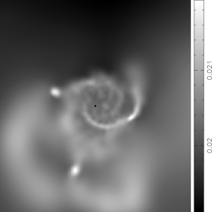
Figure 3: (a) A column-density plot of the region around a sink. The view is $500\,{\rm au}$ across, and the grey-scale bar indicates the column density in ${\rm g}\,{\rm cm}^{-3}$. The black dot at the centre indicates the position of the sink. (b) A close-up, $100\,{\rm au}$ across, of the region in the bottom middle of (a) that is about to form another sink. This shows that the particles about to form the sink (large points) have collapsed into a spherical region and are not strung out along a filament. The elongation of the region is caused by particles which are accreted shortly after sink formation (open circles).

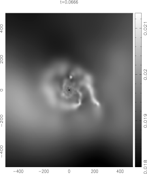
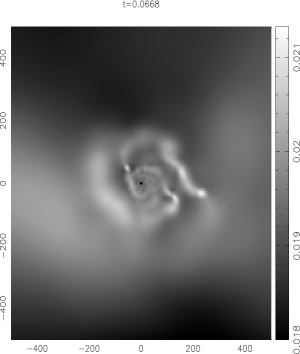
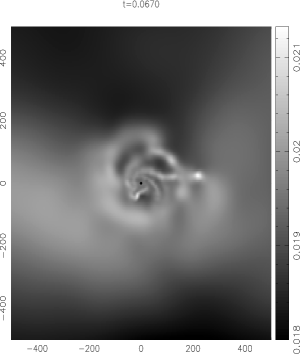
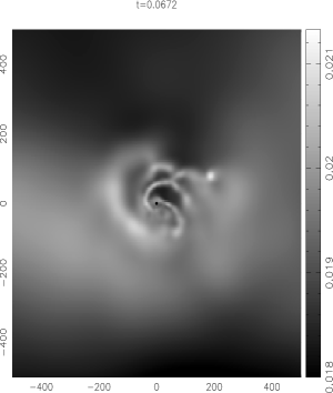
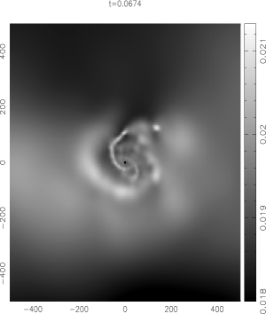
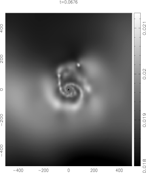
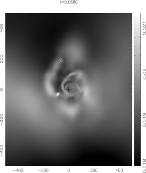
Figure 6: Column-density plots of the evolution of the region around the primary star in Run A022 as it produces a second object. Labeling is as in Fig. 5. The spiral features that are shown forming in Fig. 5 become self-gravitating and form knots along the arms. A sink condenses out of one of these knots in the last panel. This knot can be followed anti-clockwise starting from $(x,y)=(+225\,{\rm au},-100\,{\rm au})$ in the first panel.

A significant concern in low-resolution simulations is that a filament which should fragment into more than one condensation will just form a single sink. However, Fig. 3 demonstrates that, by setting $\rho_{\rm sink}=100\rho_{\rm crit}$, we ensure that an unstable region that will form a sink has condensed to an approximately spherical object prior to sink creation (see also Fig. 6). This shows that the creation of sink particles is not suppressing the fragmentation of filaments.

4 Results

The most significant results of this investigation can be summarised succinctly. First, a small level of turbulence induces the formation of multiple systems in 80% of cores. Second, the number and properties of the objects formed in an individual core depends, in a chaotic way, on the details of the initial turbulent velocity field, ranging from one object to ten with an average of 4.55 objects per core. Third, the properties of the binary and multiple systems that form are compatible with observation.

Henceforth we use the term ‘objects’ to refer to sinks formed in the simulations, and then more specifically ‘stars’ for objects with masses greater than $0.08M_{\odot}$ and ‘brown dwarfs’ for objects of lower mass.

4.1 No turbulence

To provide a reference for the turbulent simulations, we conduct 10 runs with no turbulence. Here the only difference between individual simulations is the random number used to seed the initial positions of the SPH particles. In all cores with no turbulence, only one object forms, always a star, and always within $100\,{\rm au}$ of the centre of mass. This is exactly what would be expected from the collapse of an initially static and slightly sub-virial core.

In all cases, the accretion histories of the stars are indistinguishable, An example is given in Fig. 4, which shows the mass and accretion rate of the star as a function of time. The accretion rate is initially high ($\sim 10^{-4}M_{\odot}\,{\rm yr}^{-1}$) and then drops rapidly over the course of the next $\sim 10^{5}\,{\rm yrs}\,$. The high initial accretion rate is due to material from the uniform density kernel of the core, which, having approximately uniform density, undergoes nearly freefall collapse. The accretion rate subsequently decreases as material from the lower density envelope falls inwards.

The evolution of these zero-turbulence cores follows closely the semi-analytic model of Whitworth & Ward-Thompson (2001) who assumed negligible internal pressure and hence free-fall collapse. The central density rises to the sink formation threshold of $10^{-11}\,{\rm g}\,{\rm cm}^{-3}$ after around $0.05\,{\rm Myr}$. Subsequent accretion (Fig. 4 (b)) then follows closely the pattern in Fig. 3 of Whitworth & Ward-Thompson (2000). The accretion rate at very early times is slightly in excess of the Whitworth & Ward-Thompson (2001) value due to the SPH particles having finite mass.

4.2 Turbulent cores

In order to evaluate the effect of turbulence we have conducted an ensemble of 20 simulations with $\alpha_{\rm turb}=0.05$. In Table 2 we summarise the results of these simulations, $0.3\,{\rm Myr}$ after their start. In 80% of simulations, turbulence results in the formation of multiple objects, and the number of objects that forms depends only on the detailed structure of the initial turbulent velocity field (i.e. the random-number seed that generates the turbulence). A total of 91 objects is formed in the 20 simulations, 75 stars and 16 brown dwarfs, averaging 4.55 objects per core. Each core produces between 1 and 4 high mass ($>0.5M_{\odot}$) stars, and between 0 and 8 low mass ($<0.5M_{\odot}$) objects. All but one of the brown dwarfs form in clouds that produce $\geq 6$ objects. Star formation mostly occurs between 0.05 and $0.10\,{\rm Myr}\,$, and only Run A013 undergoes star formation after $0.2\,{\rm Myr}\,$, forming 3 very low mass stars and one brown dwarf between 0.26 and 0.28 Myr.

In the main text we will limit our discussion to the general statistical properties of the ensemble of simulations. In Appendix 1 we briefly outline the evolutionary histories of the individual cores.

Table 2: A summary of the results from all 20 low-turbulence simulations. The first column gives the run identifier; the second column gives the total number of objects that form, $N_{\rm obj}$; the third column gives the total mass accreted by all of the objects in a core by $0.3\,{\rm Myr}\,$, $M^{*}_{\rm tot}$; and the fourth column gives the resulting star-formation efficiency, $\eta$. The fifth column summarises the multiplicity of the final system of objects; Run A013 has recently undergone a burst of star formation and the multiple system is very unstable at the end of the simulation. The sixth column gives the masses of individual objects, marked with a ^b, ^t or ^q if that object is part of a binary, triple or quadruple, respectively.

Run	$N_{\rm obj}$	$M^{*}_{\rm tot}/M_{\odot}$	$\eta$	Multiplicity	Masses/$M_{\odot}$
A011	7	2.94	0.54	Triple system	1.31t, 0.61t, 0.52t, 0.27, 0.12, 0.063, 0.048
A012	4	3.72	0.69	Wide binary	2.32b, 0.74b, 0.48, 0.18
A013	10	3.10	0.57	Binary + triple∗	1.07b, 0.66b, 0.43, 0.34, 0.17, 0.13t, 0.10t, 0.09t, 0.076, 0.040
A014	3	4.02	0.74	Triple system	1.63t, 1.56t, 0.83t
A015	2	3.69	0.68	Wide binary	2.63b, 1.06b
A016	3	3.61	0.67	Wide binary	2.18b, 1.40b, 0.028
A017	6	3.75	0.69	Triple system	1.60t, 1.16t, 0.64t, 0.18, 0.12, 0.050
A018	7	3.65	0.67	Triple system	1.09t, 1.03t, 0.69t, 0.58, 0.18, 0.045, 0.041
A019	8	3.81	0.70	Triple system	1.27t, 1.16t, 0.69t, 0.39, 0.21, 0.044, 0.030, 0.025
A020	1	3.63	0.67	Single star	3.63
A021	1	3.69	0.68	Single star	3.69
A022	4	4.01	0.74	Double binary	1.52q, 0.91q, 0.89q, 0.69q
A023	4	3.56	0.66	Triple system	1.43t, 0.83t, 0.70t, 0.60
A024	5	3.55	0.66	Close binary	1.46b, 1.28b, 0.43, 0.19, 0.18
A025	8	3.47	0.64	Wide binary	1.43b, 0.76b, 0.51, 0.47, 0.14, 0.064, 0.045, 0.039
A026	7	3.94	0.73	Triple system	1.23t, 1.03t, 0.73, 0.71t, 0.11, 0.098, 0.027
A027	2	3.67	0.68	Wide binary	3.19b, 0.48b
A028	1	3.35	0.62	Single star	3.35
A029	7	3.61	0.67	Double binary	1.20q, 0.89q, 0.57, 0.51, 0.29q, 0.11, 0.041q
A030	1	2.62	0.48	Single star	2.62

4.3 The origin of multiple fragmentation

The initial collapse of a core causes a significant over-density to form near the centre of the core. Usually this over-density is flattened, i.e. either layer-shaped due to the convergence of two large turbulent elements, or disc-shaped due to local spin angular momentum. This flattened region then becomes unstable and forms the first sink particle, hereafter the primary star. The initial location of the primary star is typically within $2,000\,{\rm au}$ of the centre of mass of the core; its exact position depends upon the details of the turbulent velocity field.

The primary star always forms roughly one free-fall time ($\sim 0.05\,{\rm Myrs}$) after the beginning of the simulation. The low level of turbulence invoked here is not sufficient to delay the collapse of the core significantly. This is in contrast to the high-turbulence simulation of Bate et al. (2002a,b, 2003), where turbulent energy causes the core to expand initially, and results in the formation of strong filaments.

The primary star grows rapidly in mass by accreting from the surrounding over-density. The inflow is anisotropic, being strongest in the plane of the flattened over-density, lumpy, and variable. Usually it also has net angular momentum relative to the primary star, and in this case a circum-primary disc forms. Due to the lumpy, variable accretion, these discs become unstable to spiral modes and fragment to produce secondary objects. The genesis of secondary objects is usually concentrated in a burst between 0.07 and $0.08\,{\rm Myr}$ after the start of the simulation (or 0.01 to $0.03\,{\rm Myr}$ after the primary star forms).

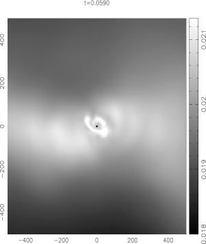
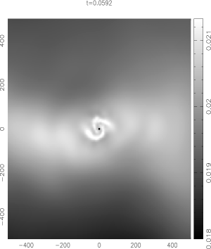
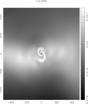
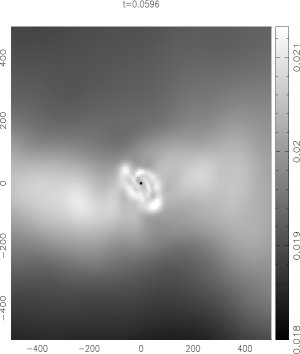
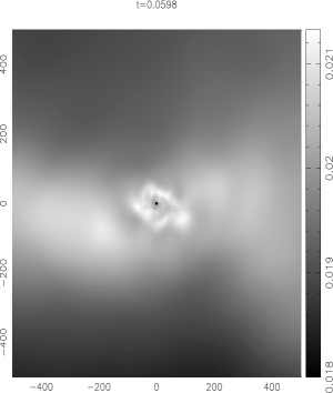
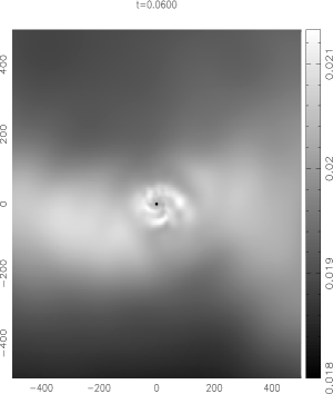
Figure 5: Column-density plots of the evolution of the region around the primary star in Run A022, showing the development of spiral features. The spatial scale of the region is given in au, and the frame is centred on the primary star. The grey-scale bar gives the column-density in ${\rm g}\,{\rm cm}^{-2}$, and the time is shown in Myr above each panel. Inflow occurs preferentially from the left and right and perturbs the disc around the primary star, exciting spiral instabilities.

The evolution of Run A022 is shown in Figs. 5 and  6, as an illustration of these processes at work. In all frames the primary star is at the centre of co-ordinates. Fig. 5 shows the lumpy accretion flow onto the primary star, concentrated preferentially through two streams on either side of the primary star. The lumpy inflow causes the disc to become unstable, forming spiral arms. Eventually one of these arms sweeps up sufficient material to detach and condense into a secondary object, as shown in Fig. 6; the knot that forms the secondary object is at $(x,y)\sim(+225{\rm au},-100{\rm au})$ in the first panel of Fig. 6, and orbits the primary anti-clockwise, ending up as a newly-formed sink at $(x,y)\sim(-80{\rm au},+200{\rm au})$ in the final panel of Fig. 6. We emphasise that this knot has already condensed out of the spiral arm that spawned it, by the time that it becomes a sink. A third sink is formed shortly after the illustrated sequence ends, from a knot that can be seen in the last three panels moving anti-clockwise from $(x,y)\sim(-50{\rm au},+100{\rm au})$ to $(x,y)\sim(-50{\rm au},-50{\rm au})$.

Not all the knots that form in this way evolve into sinks. Some are destroyed by tidal interaction and/or merger with an existing sink. An example of this can be seen in Fig. 6 where a dense knot at $(x,y)\sim(0{\rm au},+80{\rm au})$ in the first panel spirals into, merges with, the primary star.

The most significant factor in forming multiple objects appears to be the ability of the turbulent flows to create an extended overdense region in the vicinity of the primary star. The more material that is delivered into this region, the more objects that form. When an extended overdense region does not form around the primary star, the result is that no further objects form, e.g. runs A020, A021, A028 and A030.

Whilst this may appear similar to fragmentation of a disc formed from the collapse of a purely rotating cloud, there are significant differences in the scenario outlined above. Turbulence generates the angular momentum required to create a disc, but this angular momentum is provided by the turbulence in the vicinity of the first object, and not from any bulk properties of the core. It is then the clumpy, inhomogeneous inflow from the turbulent surroundings onto this disc that causes the disc to become unstable. There is no correlation between the initial angular momentum of the core and the number of objects that later form. The 3 cores with the lowest initial angular momentum (runs A013, A012 and A028)form 10, 4 and 1 objects , and the 3 cores with the highest initial angular momentum (runs A019, A014 and A016) form cores with 8, 3 and 3 objects. The amount of angular momentum varies by a factor of 4.3 between these two extremes. The differences between runs A013 and A028 are solely due to the different infall histories caused by the turbulent velocity field.

4.4 Few-body interactions and ejections

If more than two objects form in a core, the resulting ${\cal N}$-body system is generally unstable (e.g. Valtonnen & Mikkola 1991). The dynamics of unstable multiple systems are chaotic, and usually result in the ejection of low-mass members and the hardening of binaries (Anosova 1986; Sterzik & Durisen 1998).

In our simulations, this dynamical phase usually ends about 0.10 to 0.12 Myr after the start of the simulation, leaving an expanding halo of ejected objects and a central system containing between 2 and 4 stars. Simulations that produce more than two objects show a high level of dynamical instability, and no systems remain with more than 4 objects bound in the central region after $0.3\,{\rm Myr}\,$.

The timescale for dynamical evolution and ejection matches that given by Anosova (1986) who argues that systems decay on a timescale of order one hundred crossing times, i.e.

$$t_{\rm decay}\sim 0.17\,{\rm yr}\;\left(\frac{R}{\rm au}\right)^{3/2}\;\left(\frac{M}{M_{\odot}}\right)^{-1/2}$$ (7)

where $R$ is the scale-length of the system (here $\sim 200\,{\rm au}$) and $M$ is the total mass (here $\sim 2M_{\odot}$), so we obtain $t_{\rm decay}\sim 0.03\,{\rm Myrs}\,$, which is a good fit to the decay timescales we observe in the simulations.

Figure 7 shows the relationship between the velocities of the objects formed (relative to the centre of mass of the core) and their masses. The initial escape velocity from a core is $\sim 0.44\,{\rm km}\,{\rm s}^{-1}$ and this is marked by the horizontal dashed-line on Fig. 7). There is a slight anti-correlation between ejection velocity and mass. Brown dwarves have a higher mean ejection velocity ($\sim 2.9\,{\rm km}\,{\rm s}^{-1}$) than stars ($\sim 2.0\,{\rm km}\,{\rm s}^{-1}$), but this correlation is not statistically very significant.

Dynamical interactions and ejections have been proposed by Reipurth & Clarke (2001) (see also Bate et al. 2002a, Delgardo-Donate et al. 2003) as a mechanism for the production of brown dwarves: stellar embryos are ejected from cores before they can accrete enough material to become hydrogen-burning stars. This appears to be the formation mechanism for all but one of the brown dwarfs formed in these simulations. Dynamical interactions eject 36 low-mass objects from our cores, and of these 14 have not accreted enough material to pass the hydrogen-burning limit at $0.08M_{\odot}$. Only one brown dwarf is still bound in a core at $0.3\,{\rm Myr}\,$; that one is in a binary with a $0.29M_{\odot}$ star.

4.5 The mass function

Figure 8 shows the mass function of objects from all of the low-turbulence simulations at $0.3\,{\rm Myr}\,$. The filled portion of the histogram shows objects that are in multiple systems, while the open part shows single objects, and the hashed region shows the three low-mass stars which form late in Run A013; the final status of these three stars is unclear as the system is highly unstable when the simulation ends. The probability of ejection scales as $\sim M^{-1/3}$ (Anosova 1986) and ejected objects very seldom belong to multiple systems. Consequently all but one of the brown dwarfs and most of the low-mass stars are single and have been ejected (see also Fig. 7). The proportion of single stars decreases with increasing mass, because the longer a star remains in a core, the larger its mass grows, and the less likely it is to be ejected.

The low-mass tail in the mass function below $\sim 0.5M_{\odot}$ arises because secondary objects have difficulty growing beyond that mass before they are ejected. For example, the mean ejection timescale of $\sim 0.03\,{\rm Myr}$ multiplied by the mean initial accretion rate of $\sim 10^{-5}M_{\odot}\,{\rm yr}^{-1}$ gives a typical mass at ejection of $\sim 0.3M_{\odot}$. Stars with final masses greater than this are likely to be part of a central multiple system, as only in the dense central region, where accretion is on-going, can the mass grow beyond $\sim 0.5M_{\odot}$. This is shown in Fig. 8 by the high proportion of stars having $M>0.5M_{\odot}$ which are still in multiple systems at $0.3\,{\rm Myr}\,$.

The mass function shown in Fig. 8 should not be taken as a full initial mass function (IMF). It represents the statistical output from only one mass of core, with only one level of turbulence. Figure 8 is apparently deficient in low-mass objects and brown dwarfs compared with the observed IMF (e.g. Kroupa 2002). Lower mass cores may well produce the smaller objects needed to populate this region, as their gas reservoir is smaller (e.g. Delgardo-Donate et al. 2003; Sterzik & Durisen 2003). Alternatively, more turbulent cores may eject objects more rapidly, and hence with lower masses (e.g. Bate et al. 2002a,b; 2003). The true IMF is presumably a convolution of the object production from a distribution of cores masses, turbulence levels, and so on. For example, Delgardo-Donate et al. (2003) convolve the distribution of objects produced by one mass of core and one of level of turbulence with a core mass function, to produce an IMF. What is clear from these simulations is that the relationship between a core mass spectrum and a stellar IMF is non-trivial and that core mass spectra that do not resemble the stellar IMF (e.g. some of the core mass spectra from Klessen 2001) may still produce a reasonable stellar IMF.

4.6 Single stars

Four simulations produce only single stars. The turbulent velocity fields in these simulations are such that an extended overdense region does not form. The core collapses in a monolithic fashion similar to the zero-turbulence case (see Section 4.1). The only difference is that the accretion rate is somewhat lower, and the final mass at $0.3\,{\rm Myr}$ is therefore somewhat less than in the zero-turbulence case. For example, the primary star in Run A030 only reaches a mass of $2.62M_{\odot}$ by $0.3\,{\rm Myr}$, as compared with $\sim 3.75M_{\odot}$ in the runs with no turbulence. This is because the extra support provided by turbulence slows down the rate of infall onto the central sink.

4.7 Binary & multiple properties

Of the 91 objects formed, 45 remain bound in binary and multiple systems at the end of the simulations ($0.3\,{\rm Myr}$). The properties of these systems are summarised in Table 3 and also in Appendix 1.

A useful measure of the multiplicity of a stellar population is given by the companion star frequency

$${\rm CSF}=\frac{B+2T+3Q+...}{S+B+T+Q+...}$$ (8)

(Patience et al. 2002), where $S$ is the number of single stars, $B$ the number of binaries, $T$ the number of triples, etc. Summing over all the low-turbulence simulations and making no distinction between stars and brown dwarves, we have $S=46$, $B=7$, $T=6$ and $Q=2$ (plus one highly unstable quintuple system from Run A013), giving a net CSF of 0.47. Observations of older clusters and of the field give a CSF of $\sim 0.1$ (e.g. Duquennoy & Mayor 1991; Patience et al. 2002), but in young star forming regions the CSF can be far higher at 0.3 to 0.4 (Reipurth & Zinnecker 1993; Reipurth 2000; Patience et al. 2002).

The observed CSF is also very dependent on the primary mass (see Sterzik & Durisen 2003 and references therein). In our simulations, of the 41 objects having $M\leq 0.5M_{\odot}$, only 6 are in multiples, giving a low-mass CSF of $\sim 0.1$; two of these are in a binary system whose components comprise a low-mass star and a brown dwarf, and three are in the highly unstable triple produced in Run A013. Of the 50 stars having $M\geq 0.5M_{\odot}$, only 11 are not in multiple systems (and 4 of these form as single stars), giving a high-mass CSF of $\sim 0.9$. This dramatic difference between the multiplicities for low and high mass objects arises because the low-mass objects tend to have been ejected from the core early in their existence, whereas the high-mass stars stick around near the centre of mass of the core.

Table 3: The instantaneous properties of the binary and multiple systems formed in all of the low-turbulence simulations after $0.3\,{\rm Myr}\,$. The six columns give the run identifier, the primary masses, $M_{P}$, the secondary masses, $M_{S}$, the semi-major axes, $a$, the eccentricities, $e$, and the mass ratios, $q$, of the system. In higher-order multiples when one component is a binary, the primary mass is replaced by a ’B’ and the mass ratio is omitted; for example, the triple system formed in run A014 consists of an inner binary with component masses 1.63 and $0.83M_{\odot}$ and separation $12.8\,{\rm au}\,$, plus a third star of mass $1.56M_{\odot}$ orbiting the close binary at $90.6\,{\rm au}$).

Run	$M_{P}/M_{\odot}$	$M_{S}/M_{\odot}$	$a/$au	$e$	$q$
A011	1.31	0.61	6.8	0.78	0.47
A012	2.32	0.74	122	0.83	0.32
A013	1.07	0.66	22.9	0.87	0.62
A014	1.63	0.83	12.8	0.10	0.51
	B	1.56	90.6	0.09
A015	2.63	1.06	281	0.17	0.40
A016	2.18	1.40	724	0.31	0.64
A017	1.60	1.16	5.9	0.28	0.73
	B	0.64	62.2	0.07
A018	1.09	1.03	4.8	0.84	0.94
	B	0.69	205	0.81
A019	1.27	1.16	10.8	0.43	0.92
	B	0.69	78.9	0.26
A022	0.91	0.69	14.5	0.13	0.76
	1.52	0.89	12.1	0.05	0.59
	B	B	79.3	0.09
A023	1.43	0.70	4.6	0.98	0.49
	B	0.83	460	0.82
A024	1.46	1.28	18.8	0.21	0.87
A025	1.43	0.76	125	0.54	0.48
A026	1.23	1.03	4.0	0.82	0.84
	B	0.71	269	0.45
A027	3.19	0.48	170	0.15	0.15
A029	1.20	0.89	10.6	0.63	0.74
	0.29	0.041	37.6	0.33	0.14
	B	B	989	0.60

The properties of the multiple systems formed change rapidly during the early evolution of a core. The chaotic evolution of a few-body system, combined with high accretion rates and motion through a dense gas, mean that any binary properties are, at best, short-lived. Once a stable system of two to four bodies is established, the binary characteristics also tend to stabalise. All the values quoted in Table 3 are the instantaneous values at $0.3\,{\rm Myr}\,$, when the simulations were terminated. Generally the binary properties have been stable since 0.10 to $0.15\,{\rm Myr}\,$, but in simulations which form high-order multiples the orbital parameters $a$ and $e$ can change abruptly

For example, in Run A029 a binary system comprising a low-mass star and a brown dwarf encounters a high-mass central binary around $0.22\,{\rm Myr}\,$. The effect of this interaction is to harden the high-mass binary (its semi-major axis decreases from $a=61\,{\rm au}$ to $a=14\,{\rm au}$) and to throw the low-mass binary into a larger orbit ($a\sim 1000\,{\rm au}$) while also softening this binary (from $a\sim 30\,{\rm au}$ to $a\sim 40\,{\rm au}$). In Run A026, an unstable 4-body system is formed and a $0.65M_{\odot}$ star is ejected, leaving the two most massive stars in a very close binary ($a\sim 6\,{\rm au}$) with the third star orbiting at $\sim 270\,{\rm au}\,$.

The effect of ongoing accretion can be either to harden or to soften a binary. If the accretion is asymmetric, it can act to increase or decrease the velocity of the companions relative to each other, and hence change their orbital parameters. Even if the accretion is symmetric, the net effect will depend on whether the accreted gas has higher or lower specific angular momentum than the binary system (Turner et al. 1995; Whitworth et al. 1995; Bate & Bonnell 1997).

For example, in Run A012 at $0.2\,{\rm Myr}\,$, the binary components have masses of $2.07$ and $0.60M_{\odot}$ and their orbit has a semi-major axis of $18.4\,{\rm au}\,$. However, by $0.3\,{\rm Myr}\,$, the orbit has softened to $122\,{\rm au}$ and the masses have increased to $2.32$ and $0.74M_{\odot}$; accretion of gas with high specific angular momentum has caused the binary to soften. Conversely, in Run A019, accretion of gas with low specific angular momentum increases the mass ratio of the binary from $q=0.75$ to $q=0.92$ and also hardens it from $a=16\,{\rm au}$ to $a=11\,{\rm au}\,$.

While accretion can significantly affect the orbital separations of binaries, dynamical interactions appear to be the most important process generating (relatively) hard binaries in our simulations. This is shown in Fig. 9, where the semi-major axes of binaries are plotted against the total number of objects that form in a simulation. Of the 10 binaries in simulations that produce $\geq 5$ objects, 8 have $a<30\,{\rm au}\,$, compared to only 4 out of 8 binaries in simulations that produce $<5$ objects. Both simulations that only produce 2 objects (and so never have any ejections) form wide binaries with $a>100\,{\rm au}\,$.

It should be noted that for very close binary systems ($a<10\,{\rm au}$), we do not integrate the dynamics properly, due to the orbits being within the kernel-softened potential of the sinks. For this reason, the orbital parameters of close binaries are not robust. In particular, the eccentricities, and to a lesser extent the semi-major axes, are reduced by this numerical artifact

Figure 10 shows the cumulative distribution of semi-major axes from the simulations at $0.3\,{\rm Myr}\,$. The majority of binary systems have semi-major axes $a\sim 10\;{\rm to}\;20\,{\rm au}\,$, and the high-$a$ tail consists mainly of triple and quadruple systems. Also plotted in Fig. 10 is a dashed-line giving the Duquennoy & Mayor (1991) Gaussian fit to their period distribution, converted to give a distribution of semi-major axis by assuming a total system mass of $1M_{\odot}$. The distribution of semi-major axes from our simulations is consistent with that from Duquennoy & Mayor, in the sense that a KS test does not reject the sample of 26 semi-major axes as being drawn from the Duquennoy & Mayor distribution. The distribution of semi-major axes is unlikely to change significantly due to the subsequent evolution of orbital parameters, because any hardening will be counter-balanced by softening.

Figure 11 shows the cumulative distribution function of the eccentricity of multiple systems. Duquennoy & Mayor (1991) observed a roughly linear cumulative distribution for their long-period sample ($P>1000\,{\rm days}$) sample, as marked by the dashed-line, and this is consistent with our results. Duquennoy & Mayor (1991) and Mathieu (1994) found that the spread of eccentricities increases with increasing separation, but this is only significant if short-period systems ($P<1000\,{\rm days}$; $a<$ a few au) are included. We find the same trend in our results, but it is not statistically significant.

Figure 12 shows the distribution of mass ratios of the binary systems in all of the simulations, at $0.2\,{\rm Myr}\,$ and at $0.3\,{\rm Myr}\,$. In both cases, the solid histograms show hard binary systems with $a<20\,{\rm au}$, while the open histograms are for wider systems.

The mass ratios of systems are the one property that still evolves significantly in all simulations after $0.2\,{\rm Myr}$ as is clearly shown in Fig. 12. During evolution, there is a tendency for mass ratios in binary systems to become closer to unity (cf. Turner et al. 1995; Whitworth et al. 1995; Bate & Bonnell 1997). This is because the lighter companion is more able to accrete high angular momentum material, and its wide orbit through the disc gives it more chance to accrete material. For example, the close binary in Run A019 has a mass ratio of $q=0.75$ at $0.2\,{\rm Myr}$ ($M_{P}=1.06$ and $M_{S}=0.80M_{\odot}$), but by $0.3\,{\rm Myr}$ the mass ratio has risen to $q=0.92$ as the primary mass increases to $1.27M_{\odot}$ and the secondary mass increases to $1.16M_{\odot}$. As noted above this accretion also hardens the binary. Even in cases where the accretion rate onto both stars is very similar, the mass ratio increases because the proportional change in the secondary mass is greater. This results in a correlation of mass ratio with semi-major axis by $0.3\,{\rm Myr}\,$, with all 12 close systems ($a<20\,{\rm au}$) having $q>0.45$ and 5 out of 6 wide binaries ($a>20\,{\rm au}$) having $q<0.5$ (the one binary in the latter subset with $q>0.5$ only has $q=0.63$).

The distribution of mass ratios in the simulations at $0.3\,{\rm Myr}$ is close to the observed distribution, i.e. roughly linear between $q=0$ and $q=1$ (Mazeh et al. 1992, after correcting for selection effects on close binaries in the sample of Duquennoy & Mayor 1991). However, at $0.3\,{\rm Myr}$ the simulations produce fewer binaries with $q\sim 1$ than are observed by White & Ghez (2001) in Taurus-Auriga. White & Ghez (2001) do observe a correlation between binary separation and mass ratio in Taurus-Auriga, similar to that seen in Fig. 12.

5 Discussion

The main mechanism for the formation of multiple systems in dense low-turbulence cores appears to be the fragmentation of circumstellar discs. The first star to form attracts a large circumstellar disc, which is then perturbed and destabalised by non-uniform infall, and fragments to form multiple systems. These discs do not form due to the bulk angular momentum of the core, but rather because of local angular momentum in the region in which the first object forms. There is no correlation between the total angular momentum of a core and the number of objects that form in it. It is the detailed local structure of the turbulent velocity field that determines how many objects form, by first forming a circumstellar disc on scales of a few hundred au, and then by perturbing that disc due to inhomogeneous infall onto the disc.

Multiple formation occurs on the scale of a few hundred au, and the advent of high resolution sub-mm observations with instruments like ALMA will make it possible to probe this regime in unprecedented detail. The detection of highly unstable dense discs with non-axisymmetric instabilities would be a powerful confirmation of the relevance of the processes we have described above to the formation of multiple systems.

In a low-$N$ dynamical system it is unlikely that the orbits are stable and so dynamical interactions preferentially eject the low-mass members of a system (Anasova 1986). Many objects are ejected at relatively high velocity before they are able to accrete enough material to become stars, thereby producing brown dwarfs. We agree with the hypothesis of Reipurth & Clarke (2001) and Bate et al. (2002a) that an effective mechanism for the formation of brown dwarves is the ejection of protostellar embryos from their natal cores. Such a mechanism also explains the low binarity of brown dwarfs. In our simulations, only one brown dwarf is present in a multiple system.

The average ejection velocity of low mass objects is $\sim 2\,{\rm km}\,{\rm s}^{-1}$, but brown dwarves have a slightly larger average ejection velocity than low-mass stars. Also, no binary systems are ejected from cores. Thus, dynamical ejections lead to a population of low-mass objects with low binarity. The higher velocity dispersion of this population should result in mass segregation in young clusters on a relatively short timescale. Indeed, the average ejection velocity of brown dwarfs ($\sim 2$ km s^-1) exceeds the escape velocity from many small clusters. Thus, in small clusters of only a few Myrs, we would expect the spatial distribution of brown dwarves to be significantly larger than that of stars; and in older clusters the brown dwarf population may be significantly depleted by dispersion.

The companion star frequency (CSF) over our ensemble is $\sim 0.5$. This is far higher than in the field (e.g. Duquennoy & Mayor 1991), but in good agreement with the high CSF observed for young clusters and T Tauri stars of 0.3 to 0.4 (Patience et al. 2002), especially given that we do not have the selection effects which may have reduced the observed CSFs. Presumably, over time the CSF of a young stellar population is altered by the disruption of multiple systems, reducing high initial CSFs to the field value (e.g. Kroupa 1995a, b).

The CSF is very dependent upon mass, with low mass objects ($<0.5M_{\odot}$) having a CSF of only $\sim 0.1$, while more massive stars have a CSF of $\sim 0.9\,$. The huge difference between these two CSFs is due to the divide between low-mass systems which, almost by definition, are ejected from the natal core at an early stage in their growth, and high-mass systems which stick around in the centre of the natal core (interacting with the gas reservoir and with other stars) for a long time. This dependence of the CSF on mass is in the same sense as the observed decline of CSF with decreasing mass (Patience et al. 2002; Sterzik & Durisen 2003 and references therein).

The binary and higher multiple systems in our simulations have properties consistent with observations of pre-Main Sequence and Main Sequence binaries. The distribution of orbital separations is wide, between 4 and $1,000\,{\rm au}\,$, with a median semi-major axis of $\sim 30\,{\rm au}$. The distribution is consistent with a Gaussian fit to Duquennoy & Mayor’s (1991) sample of Main Sequence G-dwarves. Close binaries are formed mainly by dynamical hardening of wider binaries. The distribution of orbital separations is then further modified by accretion, which can both harden or soften existing binaries (Whitworth et al. 1995; Bate & Bonnell 1997). The distribution of eccentricities is also consistent with the observations of Duquennoy & Mayor (1991).

Mass ratios are the one binary property that evolves significantly in all of the simulations after $0.2\,{\rm Myr}\,$. At $0.2\,{\rm Myr}\,$, the mass ratios show a wide distribution with a peak in the range from $q=0.5$ to $q=0.7$. As close binaries evolve, their mass ratios tend towards higher values as (a) the lower-mass companion is more able to accrete material due to its higher angular momentum and location in the disc, and (b) even with similar accretion rates, the proportional increase in the mass of the secondary is larger (Whitworth et al. 1995; Bate & Bonnell 1997). By $0.3\,{\rm Myr}\,$, the distribution of mass ratios shows a roughly linear rise with $q$, consistent with the observations of local G-dwarfs (Duquennoy & Mayor 1991; Mahez et al. 1992). Close binaries have higher mass ratios than wide binaries; viz. all binaries with $a<20\,{\rm au}$ have $q>0.4$ by $0.3\,{\rm Myr}\,$, whereas all but one of the binaries with $a>20\,{\rm au}$ have $q<0.5\,$.

The ensemble of simulations presented in this paper represents only a single point in an extended parameter space. In future papers in this series we will examine the effect of different levels of turbulence on cores, as well as the effects of the power spectrum of the turbulence and the shape and structure of cores on star formation. We will also examine cores with different masses.

6 Conclusions

We have presented an ensemble of simulations of star formation in turbulent dense cores, using initial conditions based on observation. The cores have an initial density profile with a flat $5,000\,{\rm au}$ central region (the kernel) and an $\approx 1/r^{4}$ fall-off beyond this out to $50,000\,{\rm au}$ (the envelope). The central density is $3\times 10^{-18}\,{\rm g}\,{\rm cm}^{-3}$, and the total core mass is $5.4M_{\odot}$. The initial ratio of thermal to gravitational energy is $\alpha_{\rm therm}=0.45$.

Without turbulence, a single, central star forms, as would be expected from analytical studies (e.g. Whitworth & Ward-Thompson 2001). We then add low levels of turbulence with a low ratio of turbulent to gravitational energy of $\alpha_{\rm turb}=0.05$. The results can be summarised as follows.

• This low level of turbulence results in the formation of multiple objects in 80% of cores.

• The number of objects that forms in a turbulent core depends in a chaotic way on the details of the turbulent velocity field. Between 1 and 10 objects form in each of our 20 simulations, with an average of 4.55 objects per core.

• Close binaries ($a<20\,{\rm au}$) are formed mainly by the hardening of wider binaries due to dynamical interactions.

• The multiple systems that form in these simulations have semi-major axes, eccentricities and mass ratios compatible with the observed distributions.

• Low-mass objects ($<0.5M_{\odot}$) are often formed and then ejected from cores by dynamical interactions. This leads to a low-mass population with low binarity and high velocity dispersion.

In summary, turbulence is a fundamental ingredient of core physics, and leads to the production of abundant multiple systems. The resulting systems have properties similar to those that are observed. The levels of turbulence required to produce multiple systems are very low, similar to those observed in more quiescent isolated cores. Since the fragmentation of a turbulent core is a chaotic process, it is essential to perform a statistically significant ensemble of simulations in order to parametrize the properties of the stars which form from cores of different mass, different levels of turbulence, etc.

7 Appendix

In this appendix we describe in more detail the evolution of each of the 20 low-turbulence simulations. In all cases, unless otherwise stated, the masses quoted here are the final masses of the stars or brown dwarves at $0.3\,{\rm Myr}\,$.

7.1 A011

Seven objects form in this simulation. The first, a $1.31M_{\odot}$ star forms at $0.053\,{\rm Myr}\,$, and the other six (including two brown dwarfs) form between 0.070 and $0.073\,{\rm Myr}\,$. Four objects are ejected, and the remaining three stabalise by $0.12\,{\rm Myr}$ into a close binary (component masses 1.31 and $0.52M_{\odot}$, semi-major axis $a=9.8\,{\rm au}$) and a third relatively high-mass star ($0.61M_{\odot}$) in a distant orbit ($a\sim 800\,{\rm au}$) around this binary. As the system evolves, the central binary hardens and the more distant companion becomes only very loosely bound with an orbit of a few thousand au. Two other stars, with masses 0.27 and $0.12M_{\odot}$ are still in the core at $0.3\,{\rm Myr}\,$, but both are single.

7.2 A012

This simulation produces four stars, with masses 2.32, 0.74, 0.48 and $0.18M_{\odot}$. The first star forms after $0.056\,{\rm Myr}\,$, and the other three form in a short burst after $\sim 0.08\,{\rm Myr}\,$. At $0.15\,{\rm Myr}$ the two most massive objects form a close, eccentric binary with $a\sim 18\,{\rm au}$ and $e\sim 0.75$, but by $0.3\,{\rm Myr}$ accretion has significantly softened this binary and $a\sim 122\,{\rm au}\,$.

7.3 A013

Five stars and one brown dwarf form early in this simulation. The primary star forms at $0.052\,{\rm Myr}$ and eventually acquires a mass of $1.07M_{\odot}$. The other four stars and the brown dwarf form in a burst between 0.067 and $0.071\,{\rm Myr}\,$. By $0.20\,{\rm Myr}$, the primary star has paired up with a $0.66M_{\odot}$ star to form a close binary with $a=23\,{\rm au}$ and $e=0.87$.

An unusual second burst of star formation occurs between 0.26 and $0.28\,{\rm Myr}$, forming another four objects; by $0.3\,{\rm Myr}$, three have accreted enough material to become stars, and the fourth has been ejected as a brown dwarf. The three new stars form a very close, but highly unstable, triple, which is bound into a quintuple with the main binary system. However this quintuple is not expected to survive, and at least one of its low-mass components is likely to be ejected.

7.4 A014

Three stars form, with masses 1.63, 1.56 and $0.83M_{\odot}$, the first after $0.052\,{\rm Myr}$, and the others at $\sim 0.075\,{\rm Myr}\,$. All three stars remain bound in a triple system; the 1.63 and $0.83M_{\odot}$ stars are in a central close binary with $a=13\,{\rm au}$ and $e=0.10$, while the $1.56M_{\odot}$ star is in an orbit with $a\sim 90\,{\rm au}$ and $e=0.09$ around this binary. The outer star in the triple has been able to grow significantly faster than the central stars as, unlike those stars, it does not have to share material falling into its gravitational influence.

7.5 A015

Only two stars are formed, a $2.63M_{\odot}$ star after $0.057\,{\rm Myr}$, followed by a $1.06M_{\odot}$ star at $0.065\,{\rm Myr}$. These stars form and remain in a wide binary with $a=280\,{\rm au}$.

7.6 A016

Two stars are formed early, a $2.18M_{\odot}$ star after $0.057\,{\rm Myr}$, and a $1.40M_{\odot}$ star after $0.072\,{\rm Myr}$. The evolution is very similar to A015 until, at $0.178\,{\rm Myr}$, a third object forms and is immediately ejected as a brown dwarf.

7.7 A017

Six stars are formed, the first at $0.051\,{\rm Myr}$ and the other five in a late burst around $0.096\,{\rm Myr}$. After three stars have been ejected, a massive triple system remains, comprising a close binary (component masses 1.60 and $1.16M_{\odot}$, semi-major axis $a=6\,{\rm au}$) with a third star ($0.64M_{\odot}$) in a wide orbit with $a\sim 60\,{\rm au}$ around this binary.

7.8 A018

Five stars and two brown dwarfs are formed, the first star at $0.055\,{\rm Myr}$, the other four stars and one brown dwarf between 0.065 to $0.071\,{\rm Myr}$; the second brown dwarf forms at $0.10\,{\rm Myr}$ and is immediately ejected. Three of the stars form a triple with component masses 1.09, 1.03 and $0.69M_{\odot}$, but it is very unstable. At $0.20\,{\rm Myr}$ the two most massive stars are in a close binary, with the $0.69M_{\odot}$ star in a more distant orbit. Then at $0.21\,{\rm Myr}$ there is an interaction which swaps the $0.69M_{\odot}$ star with one of the components of the close binary, and at around $0.26\,{\rm Myr}$ they are swapped back. In addition there is a $0.58M_{\odot}$ star very loosely bound to the triple system.

7.9 A019

This simulation produces eight objects, five stars and three brown dwarves. The first object forms after $0.057\,{\rm Myr}$, followed by two bursts, the first of which forms four objects at $\sim 0.064\,{\rm Myr}$, and the second of which forms three objects at $\sim 0.090\,{\rm Myr}$. By the end of the simulation there is a massive triple comprising a close binary (component masses 1.27 and $1.16M_{\odot}$, semi-major axis $a=11\,{\rm au}$, eccentricity $e=0.43$) with a third star ($0.69M_{\odot}$) in a wide orbit ($a\sim 80\,{\rm au}$) around this binary.

7.10 A020

A single star is formed at $0.055\,{\rm Myr}$ and reaches a mass of $3.63M_{\odot}$ by $0.3\,{\rm Myr}$.

7.11 A021

A single star is formed at $0.054\,{\rm Myr}$ and reaches a mass of $3.69M_{\odot}$ by $0.3\,{\rm Myr}$.

7.12 A022

Four stars are formed in this simulation, the first after $0.057\,{\rm Myr}$, and the other three in a burst around $0.072\,{\rm Myr}$. All four stars remain bound at $0.3\,{\rm Myr}$ as an hierarchical quadruple consisting of a pair of close binary systems. The more massive binary comprises 1.52 and $0.89M_{\odot}$ stars in an orbit with $a=15\,{\rm au}$ and $e=0.13$. The less massive binary comprises 0.91 and $0.69M_{\odot}$ stars in an orbit with $a=12\,{\rm au}$ and $e=0.05$. The two binary systems are in a wide orbit around each other with $a\sim 80\,{\rm au}$ and $e\sim 0.09$.

7.13 A023

Four stars form in this simulation. The primary star forms at $0.055\,{\rm Myr}$ and eventually acquires a mass of $1.43M_{\odot}$. The remaining three stars form between 0.069 and $0.079\,{\rm Myr}$. By $0.3\,{\rm Myr}$ there is a massive triple comprising a close binary (component masses 1.43 and $0.70M_{\odot}$, semi-major axis $a=5\,{\rm au}$) with a third star ($0.83M_{\odot}$) in a wide orbit around this binary. The fourth star has $0.60M_{\odot}$ and has been ejected with a large disc early in the interaction process.

7.14 A024

Five stars are formed, the first at $0.053\,{\rm Myr}$, and the rest between 0.070 and $0.076\,{\rm Myr}$. Three of the stars are ejected, leaving a close binary with component masses $1.46$ and $1.28M_{\odot}$, semi-major axis $a=19\,{\rm au}$ and eccentricity $e=0.21$. Unusually, the most massive star at the end of the simulation is the second object to form, rather than the first as in all other simulations.

7.15 A025

Eight objects are formed in this simulation, including three brown dwarves. The primary star forms at $0.053\,{\rm Myr}$, and five further objects, including the three brown dwarves, form in a burst around $0.064\,{\rm Myr}$; the final two stars form at $0.09\,{\rm Myr}$. Five objects are ejected almost immediately, leaving a triple system, which, despite the ejections is very loose; the main binary has $a\approx 220\,{\rm au}$. After $0.17\,{\rm Myr}$ the third component of the triple is ejected and the remaining binary is somewhat hardened to $a\sim 125\,{\rm au}$.

7.16 A026

Six stars and one brown dwarf are formed. The primary star forms at $0.055\,{\rm Myr}$, and four further stars and the brown dwarf form in a burst around $0.071\,{\rm Myr}$; the final star forms at $0.092\,{\rm Myr}$. Two stars and the brown dwarf are ejected, leaving two close binaries in an hierarchical quadruple. The more massive binary comprises 1.03 and $0.71M_{\odot}$ stars in an orbit with $a=15\,{\rm au}$. The less massive binary comprises 0.73 and $0.71M_{\odot}$ stars in an orbit with $a=16\,{\rm au}$. The two binary systems are in a wider orbit around each other with $a\sim 180\,{\rm au}$ and $e\sim 0.09$. However, this system is unstable, and at $0.24\,{\rm Myr}$ the $0.73M_{\odot}$ star is ejected in a 4-body encounter, leaving the more massive binary hardened to $a=4\,{\rm au}$ (below our ability to resolve the dynamics properly) and the $0.71M_{\odot}$ star in a $270\,{\rm au}$ orbit around this binary, i.e. an hierarchical triple.

7.17 A027

Only two stars are formed in this simulation. The primary star is formed at $0.057\,{\rm Myr}$ and ends up with $3.19M_{\odot}$. The secondary star forms at $0.142\,{\rm Myr}$ and ends up with $0.48M_{\odot}$. They form a wide binary system with $a=170\,{\rm au}$ and $e=0.15$. The large mass ratio is due to the very late formation time of the secondary star and its distance from the primary.

7.18 A028

A single star is formed at $0.055\,{\rm Myr}$ and reaches a mass of $3.35M_{\odot}$ by $0.3\,{\rm Myr}$.

7.19 A029

A total of seven objects is formed, the first at $0.057\,{\rm Myr}$, another five in a burst around $0.064\,{\rm Myr}$, and a final object at $0.081\,{\rm Myr}$. Three stars are ejected, leaving two close binary systems in an hierarchical quadruple. The more massive binary comprises 1.20 and $0.89M_{\odot}$ stars in an orbit with $a=11\,{\rm au}$ and $e=0.63$. The less massive binary comprises 0.29 and $0.041M_{\odot}$ stars in an orbit with $a=38\,{\rm au}$ and $e=0.33$; this is the only example of a brown dwarf in a binary or multiple system in all our simulations. The two binary systems are in a very wide orbit around each other with $a\sim 1500\,{\rm au}$.

7.20 A030

A single star is formed at $0.055\,{\rm Myr}$ and reaches a mass of $2.62M_{\odot}$ by $0.3\,{\rm Myr}$.

Figure 1: The density profile of a prestellar core with a flat inner region (kernel) and a $1/r^{4}$ decline in the outer envelope.

Figure 2: The ratio of turbulent to gravitational energy $\alpha_{\rm turb}$ plotted against mass, for observed starless cores from Jijina et al. (1999). Also marked are the point in parameter space treated by our simulations (the star symbol) and that treated by Bate et al. (2002a,b, 2003; the open circle).

   

   

Figure 4: Left: the mass of the single star that forms in a core with no turbulence, as a function of time. Right: the accretion rate as a function of time for the same star. The accretion rate is in good agreement with the semi-analytic model of Whitworth & Ward-Thompson (2001).

  

  

  

  

  

  

  

  

Figure 7: The velocities of ejected stars plotted against their masses. The dashed-line at $0.44\,{\rm km}\,{\rm s}^{-1}$ shows the initial escape speed from the core. Brown dwarves have a higher velocity than low-mass stars after being ejected. The maximum mass of ejected stars is $\sim 0.5M_{\odot}$.

Figure 8: The mass function of stars created in the 20 low-turbulence simulations. Filled bins show objects in binary or multiple systems, while open bins show single objects. The three low-mass objects which are partially shaded are the three objects that formed late in Run A013; these objects are bound but highly unstable when the simulation is terminated at $0.3\,{\rm Myr}$, and their future evolution is therefore uncertain.

Figure 9: The total number of objects formed in a simulation $N_{\rm obj}$ plotted against the semi major axis of any binary systems formed in that simulation. Simulations which produce a large number of objects tend to produce harder binary systems.

Figure 10: The cumulative distribution function of semi-major axes for the systems formed in the 20 low-turbulence simulations. The dashed line is the Gaussian fit to the G-dwarf period distribution from Duquennoy & Mayor (1991), adjusted to be a fit to the semi-major axis distribution by adopting a system mass of $M_{\odot}$. A KS test shows the two distributions to be compatible.

Figure 11: The cumulative distribution function of eccentricities for the systems formed in the 20 low-turbulence simulations. The dashed line is the linear fit from Duquennoy & Mayor (1991), and is compatible with the simulations.

$T=0.2$ Myr

$T=0.3$ Myr

Figure 12: The distribution of binary mass ratios at $0.20\,{\rm Myr}$ and $0.30\,{\rm Myr}$ for the binary systems that form in the 20 low-turbulence simulations. The filled bins show the mass ratios for close binaries ($a<20\,{\rm au}$), and the empty bins show the mass ratios for wide binaries ($a>20\,{\rm au}$). It should be noted that one binary system at $0.20\,{\rm Myr}$ has been disrupted by $0.30\,{\rm Myr}$, resulting in one less pair in the second histogram.