First Planet Confirmation with a Dispersed Fixed-Delay Interferometer

Abstract

The Exoplanet Tracker is a prototype of a new type of fibre-fed instrument for performing high precision relative Doppler measurements to detect extra-solar planets. A combination of Michelson interferometer and medium resolution spectrograph, this low-cost instrument facilitates radial velocity measurements with high throughput over a small bandwidth ($\sim 300$Å), and has the potential to be designed for multi-object operation with moderate bandwidths ($\sim$ 1000Å). We present the first planet detection with this new type of instrument, a successful confirmation of the well established planetary companion to 51 Peg, showing an rms precision of $11.5\rm ms^{-1}$ over five days. We also show comparison measurements of the radial velocity stable star, $\eta$ Cas, showing an rms precision of $7.9\rm ms^{-1}$ over seven days. These new results are starting to approach the precision levels obtained with traditional radial velocity techniques based on cross-dispersed echelles. We anticipate that this new technique could have an important impact in the search for extra-solar planets.

1 INTRODUCTION

Of the more than one hundred extra-solar planets that have been found to date, the vast majority have been found using the radial velocity (RV) technique (e.g. Butler et al. (1996); Baranne et al. (1996)). Current approaches to making RV measurements rely on using very high resolution echelle spectrographs, employing cross-correlation or fits to line profiles in stellar spectra to determine Doppler shifts in the centroids of the lines. While the RV technique has been the most successful technique for locating extra-solar planets, traditional echelles have relatively low light throughput, large instrument volume, and tend to be very expensive. In addition, they cover only a single object in each observation. The low light throughput limits survey sensitivity to relatively bright stars and single object operation leads to slow survey speeds.

The Exoplanet Tracker (ET) is a prototype of a new type of fibre-fed RV instrument based on a dispersed fixed-delay interferometer, a combination of a Michelson interferometer followed by a low or medium resolution post-disperser. This combination has been suggested for spectroscopic applications as early as the 1890’s (Edser & Butler, 1898), and was proposed for precision Doppler planet searches by D. J. Erskine in 1997 (Erskine & Ge, 2000; Ge, Erskine, & Rushford, 2002); a similar approach is discussed in Mosser, Maillard, & Bouchy (2003). The effective resolution of the instrument is determined primarily by the interferometer, so the post-dispersing spectrograph can be of much lower resolution than in traditional techniques, and consequently can have much higher throughput (Ge, 2002; Ge et al., 2003a, b).

The cost of the instrument is comparitively low, and furthermore it operates in a single-order mode: a single spectrum only takes up one strip along the CCD detector. Spectra from multiple stars can be lined up at once on a single detector to increase survey speed (Ge, 2002). In combination with a wide field multi-fibre telescope, multi-object surveying should therefore be achievable (Mahadevan et al., 2003), with the potential to rapidly increase the number of known extra-solar planets.

The instrument works by producing a long-slit stellar spectrum ‘channeled’ with fringes, also known as Edser-Butler fringes (Edser & Butler, 1898; Lawson, 2000; Ge, 2002). Sinusoidal interference fringes are formed along the slit direction wherever there are spectral lines. Doppler shifts in the underlying spectrum result in directly proportionate phase shifts in these fringes. Hence, we measure shifts of the sinusoids in the slit direction, rather than shifts of the spectrum itself in the dispersion direction as in traditional techniques. By fitting sine functions to the CCD response along each wavelength channel on the detector and combining the results from all channels, we are able to accurately measure any changes in the Doppler shift of an object. The concept is described in more detail in Ge (2002); van Eyken et al. (2003).

In this paper, we report Doppler RV curves of the known planet-bearing star, 51 Peg (Mayor & Queloz, 1995), and a RV stable star, $\eta$ Cas with ET at the KPNO 2.1m telescope. This represents the first planet detection using this independent new technique.

2 OBSERVATIONS

The observations were conducted with a prototype of ET during an engineering run at the KPNO 2.1m telescope in August 2002, built largely from cheap off-the-shelf components. The observations and details of the instrument setup were reported in Ge et al. (2003a).

The spectrograph operating resolution was measured at $R\approx 4540$. Using a KPNO 1k$\times$3k back-illuminated CCD gave a wavelength coverage of $\sim 270$Å centred around 5445Å. The image was spread over $\sim 300$ pixels in the slit direction, giving a total of around 12 periods of fringing. An iodine vapour cell was inserted into the beam as a Doppler zero velocity reference, with its temperature stabilised to $60\pm 0.1^{\circ}{\rm C}.$

During the run, we were able to obtain regular observations of a number of stars, including known planet bearing stars 51 Peg, $\upsilon$ And and HD209458; RV stable stars $\eta$ Cas, $\tau$ Ceti and and 31 Aql; and a bright star, $\alpha$ Boo, over a period of about seven days (Ge et al., 2003a). In this paper, only results from 51 Peg and $\eta$ Cas are reported.

3 DATA ANALYSIS

Raw spectra were first trimmed and dark subtracted using standard IRAF routines, with bias being subtracted along with the darks in one step. Pixel-pixel flatfielding was performed using non-fringing quartz-lamp continuum spectra as flatfields, where the fringes were eliminated by rapidly oscillating the interferometer PZT mirror during the exposure.

The rest of the data reduction was then performed using custom software written in the IDL data analysis language, by Research Systems Inc. Images were ‘self illumination corrected’ using an algorithm to extract the underlying continuum illumination function from each image, which is divided out. This avoids problems with changes in the illumination over time. The spectra were then corrected for slant so that the slit direction was exactly aligned with the CCD pixel axes. They were then low-pass Fourier filtered in order to remove the interferometer comb, the series of parallel fringes that would be present if pure white light were to be observed and which contains no Doppler information itself.

After these pre-processing steps, the phase and visibility were determined for each wavelength channel by fitting a sin wave to each column of the CCD image, each pixel being weighted according to the number of counts in the original non-flatfielded data on the assumption of photon noise dominated error. Since fringe spatial frequency varies only slowly as a function of wavelength, we fit a smooth function to the frequencies obtained from the sinusoid fits, and then performed a second pass with the frequencies fixed to match this function, helping to reduce random errors.

To a good approximation, the combined iodine/star data frames can be considered a linear summation of the complex visibilities of the individual iodine and stellar spectra (where complex visibility is defined as ${\bf V}=Ve^{i\phi}$, with $V$ the fringe visibility and $\phi$ the phase offset). Pure stellar and pure iodine template spectra were taken at the beginning of each observation, and these were used to mathematically extract the phase shifts of the star and the iodine individually, and hence calculate the intrinsic stellar velocity shift corrected for instrumental drifts.

Finally, the RV due to the motion of the Earth was subtracted to leave an intrinsic stellar relative velocity curve. Currently the exposure time is taken to be the centre of the exposure (although this is by no means necessarily ideal).

Error bars are based on the standard statistical curve-fitting errors determined during measurement of phase and visibility. The errors are translated to error bars through calculations appropriate to the algorithms used to extract the final intrinsic stellar RV. They are expected to give a reasonable guide to the random scatter expected in the data, although they may not catch all systematic errors.

On closer inspection, the data were found to show variation in the fringe phase and visibility along the length of the slit. We therefore cut the spectra into three slices along the dispersion direction and treated each slice separately, in order to obtain sinusoidal fits less affected by this systematic error. A weighted average of the three results was then obtained to give a final RV plot.

4 RESULTS

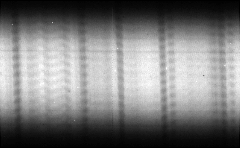
Figure 1: Raw fringing spectrum of 51 Peg with iodine, obtained at KPNO on the night of 2002 Aug 14. (mag 5.5, S/N$\sim 50$ per pixel)

Part of the raw fringing spectrum for 51 Peg with the overlayed iodine spectrum is shown in figure 1, obtained in 25 minutes at visual magnitude 5.5 with S/N per pixel in the central strip of around 50. Typical exposure times for $\eta$ Cas (mag 3.5) were 30 min at an S/N of 80 (including iodine cell losses).

Figure 2 shows the radial velocity variation measured for 51 Peg after diurnal motion is subtracted. The zero point is chosen arbitrarily. Over-plotted is the expected curve extrapolated from the most recently determined orbital parameters (Naef et al., 2003). The same data are listed in table 1. S/N per pixel ratios obtained were in the range $\sim$40–60 for star+iodine spectra. The templates used for the processing are from the night of August 16 (August 17 UT), and S/N for the iodine and star templates were approximately 300 and 70 per pixel respectively (for the central strip). Averaging over the three detector strips gives an rms deviation from the predicted curve of $11.5\rm ms^{-1}$. The value of the reduced $\chi^{2}$ is 2.70.

Residuals after diurnal correction for the star $\eta$ Cas are shown in figure 3 and table 2, using templates from the night of Aug 15 (Aug 16 UT). $\eta$ Cas is a known RV stable star (W. D. Cochran 2002, private communication) and is therefore expected to show zero shift at our current level of precision. The three image strips are averaged, weighted according to flux. The rms scatter is $7.9\rm ms^{-1}$, with a reduced $\chi^{2}$ of 2.03. Typical S/N per pixel in the central strip is around 70–90 for star+iodine spectra, 270 for the iodine template, and 100 for the star template.

Under 1.5 arc-sec seeing conditions, we obtained a total instrument throughput of $\sim 4\%$, from above the atmosphere to the detector, including sky, telescope transmission, fibre loss, instrument and iodine cell transmission, detector quantum efficiency, and using only one interferometer output. Excluding slit loss, the transmission of the instrument itself from fibre to detector was 19%.

5 DISCUSSION

It is possible to make an estimate of the photon limited error for this instrument using the following analysis. Following Ge (2002), the error $\sigma_{i}$ in velocity from a single wavelength channel $i$ due to photon noise alone can be calculated as a function of fringe visibility, $\gamma_{i}$, and total photon flux in the channel, $F_{i}$. Using a slightly more accurate derivation than given in Ge (2002) gives the relation:

$$\sigma_{i}=\frac{c\lambda}{\pi d\gamma_{i}\sqrt{2F_{i}}},$$ (1)

where $c$ is the speed of light, $\lambda$ is the operating wavelength, and $d$ is the path difference between the interferometer arms. The combined error over all channels is then given by:

$$\sigma=[\sum_{i}1/\sigma_{i}^{2}]^{-\text@frac{1}{2}}.$$ (2)

This gives us an estimate of the error due to the photon noise in one complete fringing spectrum. In order to estimate the photon error for the final iodine reference corrected RV measurement, we must combine the errors from the templates, $\sigma_{\rm I_{2},template}$ and $\sigma_{\rm star,template}$, and from the combined star+iodine data. We treat the combined data as consisting of two separate components, with errors $\sigma_{\rm I_{2},data}$ and $\sigma_{\rm star,data}$. The final relative velocity measured, $V$, is given by $V=(V_{\rm star,data}-V_{\rm star,template})-(V_{\rm I_{2},data}-V_{\rm I_{2},template})$, and so the final error is obtained by quadrature addition:

$$\sigma_{V}^{2}=\sigma_{\rm star,data}^{2}+\sigma_{\rm star,template}^{2}+\sigma_{\rm I_{2},data}^{2}+\sigma_{\rm I_{2},template}^{2}.$$ (3)

We find the errors due to the templates using equations 1 and 2. To find the errors $\sigma_{\rm I_{2},data}$ and $\sigma_{\rm star,data}$, we take the errors calculated for the templates, and scale these to find the values that they should have at the S/N of the data, noting from equation 1 that the errors scale as the reciprocal of S/N (where S/N$=\sqrt{F}$).

The results of these calculations are shown in table 3. We find final photon limiting precisions (averaged over all data points) of $11.0\rm ms^{-1}$ for 51 Peg and $8.1\rm ms^{-1}$ for $\eta$ Cas. Within the uncertainty in the rms residual values obtained for the data due to the small number of data points ($11.5\pm 2.1\rm ms^{-1}$ for 51Peg and $7.9\pm 1.2\rm ms^{-1}$ for $\eta$ Cas), we find a good match with the data and conclude that we have reached the photon limit: the reduction software has successfully extracted the maximum possible information from the data. It is important to note, however, that these values for the photon limit are those expected given the fringe visibility that was obtained. Various instrument effects (for example defocus) can reduce the visibility from its optimum and hence reduce the precision. It is therefore possible that the intrinsic limit is somewhat lower for an ideally optimised instrument.

We note the large contribution to the errors due to the iodine reference. Though the iodine can be measured to very high accuracy for the template since a quartz lamp is used for illumination, the iodine in the combined star/iodine images has much lower S/N, and this becomes an important source of error. In both the 51 Peg and the $\eta$ Cas cases, the error due to the iodine is comparable to that of the star itself.

Given this photon limit, the error bars in the data appear to be underestimated (leading to the large values for the reduced $\chi^{2}$). A possible cause of this is the low pass Fourier filtering that is done to remove the interferometer comb. In addition to removing the comb, filtering has the effect of smoothing the photon noise in the data, reducing the residuals in the sinusoid fits to the fringes and thereby reducing the resulting error estimates for each fringe. This may be an artificial effect, however, which in fact does not improve the precision of the fits. The extent to which this effect occurs is under investigation.

6 CONCLUSION

We have achieved $11.5\rm ms^{-1}$ RV precision over five days of observations of 51 Peg, obtaining results in excellent agreement with previously measured orbital parameters due to its planetary companion. We have also obtained measurements of a RV stable star, $\eta$ Cas, showing that we can reach a precision of $7.9\rm ms^{-1}$ over seven days, using a simple and inexpensive prototype. The rms residuals match the expected photon limited errors for the instrument, given the fringe visibilities obtained, and show that the precision we are able to obtain with ET is becoming comparable with current traditional echelle techniques. For comparison, rms scatters obtained previously for 51 Peg have been $13\rm ms^{-1}$(Mayor & Queloz, 1995), $5.2\rm ms^{-1}$ (Marcy et al., 1997), and $11.8\rm ms^{-1}$ (Naef et al., 2003).

Table 1: RV measurements for 51 Peg

JD	Velocity	Error
$-2450000$	$(\rm ms^{-1})$	$(\rm ms^{-1})$
$2500.8665$	$35.4$	$7.1$
$2500.8879$	$46.8$	$6.8$
$2500.9094$	$29.4$	$6.8$
$2501.9077$	$18.1$	$6.8$
$2501.9263$	$30.8$	$7.0$
$2501.9441$	$29.9$	$7.0$
$2502.9392$	$-78.1$	$8.4$
$2502.9573$	$-61.6$	$8.3$
$2502.9751$	$-57.9$	$7.8$
$2503.9250$	$-50.9$	$6.7$
$2503.9480$	$-57.9$	$6.8$
$2503.9692$	$-27.6$	$6.6$
$2504.8960$	$44.2$	$6.5$
$2504.9177$	$28.1$	$6.6$
$2504.9392$	$15.4$	$6.8$

Table 2: RV measurements for $\eta$ Cas

JD	Velocity	Error
$-2450000$	$(\rm ms^{-1})$	$(\rm ms^{-1})$
$2498.8318$	$6.4$	$5.7$
$2498.8545$	$8.3$	$5.1$
$2498.8823$	$-11.2$	$5.4$
$2498.8936$	$10.9$	$5.3$
$2499.7839$	$6.8$	$6.3$
$2499.7952$	$2.9$	$6.0$
$2499.8064$	$-3.6$	$5.8$
$2499.8174$	$1.7$	$5.8$
$2499.8284$	$1.4$	$5.9$
$2501.8701$	$-5.9$	$5.3$
$2501.8777$	$-9.6$	$5.4$
$2501.8850$	$-15.3$	$5.5$
$2501.8926$	$7.7$	$5.4$
$2502.8528$	$-0.0$	$4.9$
$2502.8643$	$-1.7$	$4.9$
$2502.8752$	$5.4$	$5.1$
$2502.8860$	$-10.8$	$5.4$
$2504.8093$	$-1.4$	$5.7$
$2504.8201$	$-10.1$	$6.4$
$2504.8311$	$2.5$	$5.4$
$2504.8401$	$11.7$	$5.9$

Table 3: Mean photon limited error estimation

Component	Star	Iodine
	($\rm ms^{-1}$)	($\rm ms^{-1}$)
51 Peg
Templates	4.7	1.2
Data	6.7	7.2
Combined	11.0
$\eta$ Cas
Templates	4.2	1.2
Data	5.3	4.3
Combined	8.1

Figure 2: Radial velocity measurements for 51 Peg, with the predicted curve over-plotted. RMS residuals are $11.5\rm ms^{-1}$.

Figure 3: RV measurements for $\eta$ Cas, an RV stable star, expected to show zero shift. RMS residuals are $7.9\rm ms^{-1}$.

References

- Baranne et al. (1996) Baranne, A. et al. 1996, A&AS, 119, 373
- Butler et al. (1996) Butler, R. P., Marcy, G. W., Williams, E., McCarthy, C., Dosanjh, P., & Vogt, S. S. 1996, PASP, 108, 500
- Edser & Butler (1898) Edser, E. & Butler, C. P. 1898, Phil. Mag., 46, 207
- Erskine & Ge (2000) Erskine, D. J. & Ge, J. 2000, ASP Conf. Ser. 195: Imaging the Universe in Three Dimensions, 501
- Ge (2002) Ge, J. 2002, ApJ, 571, L165
- Ge, Erskine, & Rushford (2002) Ge, J., Erskine, D. J., & Rushford, M. 2002, PASP, 114, 1016
- Ge et al. (2003a) Ge, J., van Eyken, J. C., Mahadevan, S., DeWitt, C., Ramsey, L. W., Shaklan, S. B., & Pan, X. 2003a, Proc. SPIE, 4838, 503
- Ge et al. (2003b) Ge, J., Mahadevan, S., van Eyken, J., DeWitt, C., & Shaklan, S. 2003b, in ASP Conf. Ser. 294, Scientific Frontier in Research in Extrasolar Planets, ed. Deming, D., & Seager, S. (San Fransico: ASP), 573
- Lawson (2000) Lawson, P. R. 2000, in Principles of Long Baseline Stellar Interferometry, ed. P. R. Lawson (Pasadena: JPL Publications), 113
- Mahadevan et al. (2003) Mahadevan, S., Ge, J., van Eyken, J. C., DeWitt, & Shacklan, S. 2003, Proc. SPIE, in press
- Marcy et al. (1997) Marcy, G. W., Butler, R. P., Williams, E., Bildsten, L., Graham, J. R., Ghez, A. M., & Jernigan, J. G. 1997, ApJ, 481, 926
- Mayor & Queloz (1995) Mayor, M. & Queloz, D. 1995, Nature, 378, 355
- Mosser, Maillard, & Bouchy (2003) Mosser, B., Maillard, J., & Bouchy, F. 2003, PASP, 115, 990
- Naef et al. (2003) Naef, D., Mayor, M., Beuzit, J. L., Perrier, C., Queloz, D., Sivan, J. P., Udry, S. 2003, A&A, in press
- van Eyken et al. (2003) van Eyken, J. C., Ge, J., Mahadevan., S., DeWitt, C., & Ren, D. 2003, Proc. SPIE, in press