Numerical simulations of self-gravitating magnetized disks

Abstract

We present the first global simulations of self-gravitating magnetized tori. The simulations are performed with Zeus-2D and GLOBAL. We find the magnetorotational instability (MRI) to behave similarly in a self-gravitating environment as in previous simulations of non self-gravitating systems: enhancement of turbulent angular momentum transport follows the linear phase. The torus quickly develops a two component structure composed of an inner thick disk in Keplerian rotation and an outer massive disk. We compare this result with zero mass global simulations in 2D, and also present preliminary results of 3D simulations.

1 Introduction

In the early phases of star formation, the forming accretion disks are likely to be very massive because of a strong infall from the parent molecular cloud. These massive disks are subject to the development of gravitational instabilities which redistribute angular momentum [Laughlin et al. (1998)]. However, when sufficiently ionized, the disks are also unstable to the MRI [Balbus & Hawley (1991), Balbus & Hawley (1998)]. The simultaneous development of both instabilities in these disks may significantly affect their evolution. We have therefore undertaken a numerical study of this phenomenon by means of numerical simulations of self-gravitating magnetized tori.
In section 2, we present a summary of our numerical methods, and describe the initial equilibrium configuration. In section 3, we present the results of the 2D simulations, and compare them with nonself-gravitating tori evolution. In section 4, we review preliminary results obtained in 3D, and we discuss the future developments of this work in section 5.

2 Numerical methods

2.1 Algorithms

We used the code Zeus-2D [Stone & Norman (1992a,b)] to perform the axisymmetric calculations in cylindrical coordinates. Zeus-2D solves the MHD equations using time-explicit Eulerian finite differencing. Magnetic fields are updated with the Constrained Transport method [Evans & Hawley (1988)] in order to preserve $\nabla\cdot\vec{B}=0$ and the method of characteristics is used to compute the electromotive forces in order to accurately describe the propagation of Alfven waves. The Poisson solver in Zeus-2D has been modified and involves two steps. We first calculate the gravitational potential $\phi_{g}$ on the boundary, using the Legendre functions well-suited to our cylindrical geometry [Cohl & Tohline (1999)], and we then apply the Successive Over-Relaxation method to update $\phi_{g}$ everywhere on the grid [Hirsch (1988)]
For the 3D simulations, we have used the code GLOBAL [Hawley & Stone (1995)], a 3D MHD solver that uses Eulerian finite-differencing similar to Zeus 2D. This code was modified to include a 3D version of the Poisson solver described above.

2.2 Initial configuration

Building an equilibrium self-gravitating torus is not completely straightforward, because the density and gravitational potential influence each other. A change in the density field modifies the gravitational potential which in turns affects the density and so on. This suggests the use of an iterative method. We used the self-consistent field method developed by hachisu86.
Our typical model parameters are those of a torus, with the inner and outer radii at $R_{in}=0.3$ and $R_{out}=1$ respectively. The angular velocity profile is a power law: $\Omega\propto r^{-1.68}$ and we add a central mass $M_{c}$ such that $M_{c}/M_{d}=0.5$, $M_{d}$ being the torus mass. Finally, we normalized the density such that $\rho_{max}=1$.
In the following, we compare the evolution of this torus to its zero mass counterpart. The above parameters are identical in the two cases, but the gravitational potential in the latter is that of the central mass. This gives a density field similar to that of the self-gravitating model, but lowers the pressure by about an order of magnitude.

3 2D simulations

In this section, we describe the results of the simulations performed in 2D with a resolution in $(R,z)=(256,256)$. A weak poloidal magnetic field is added to the model describe above, with the toroidal component of the vector potential being:

$$A_{\phi}\propto\rho\times\cos\left(2\pi\frac{R-R_{in}}{R_{out}-R_{in}}\right)$$ (1)

The components of the magnetic field are then scaled such that the volume averaged ratio of magnetic to thermal pressure (hereafter called $\beta$) equals $1500$ for the self-gravitating model and $200$ for the zero mass one.
We found the MRI grows in both models, developing approximately the same Maxwell stress. In the self-gravitating case, the evolution is very similar to what was found before (see for example hawley00): the early linear growth of the instability is followed by a turbulent phase during which angular momentum is transported outward. Turbulence then gradually decays because of the anti-dynamo theorem. During this phase, the vertically averaged Maxwell stress tensor $T_{R\phi}^{Max}=-\langle B_{R}B_{\phi}/4\pi\rho\rangle$ is dominant over the Reynolds stress $T_{R\phi}^{Rey}=\langle v_{R}\delta v_{\phi}\rangle$.

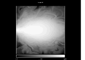
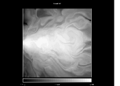
a. Self-gravitating torus after 5.8 orbits b. Zero mass torus after 5.2 orbits

Figure 1: Comparison between the density logarithm distribution in the ($r$-$z$) plane for the self-gravitating torus (left panel) and the zero mass torus (right panel). The former develops a two-component structure composed of an inner Keplerian disks and an outer, more massive, thick disk. The later is disrupted by the MRI, and a standard thin disk structure builds up, with a constant $H/R$ ratio.

Figure 2: Angular momentum profile in the equatorial profile of the torus, averaged between orbits 5.05 and 7. The dashed shows the Keplerian profile resulting from the central point mass, the dotted line has a power law dependance on the radius: $l\propto r^{0.9}$.

We show in figure 1 the logarithm of the density field in the $(r-z)$ plane during the turbulent phase for both models. In the self-gravitating case (left panel), the initial torus has developed a two-component structure, composed of an inner thin disk fed by an outer thick and massive torus. Figure 2 shows the angular momentum radial profile in the equatorial plane during this phase (solid line). As shown by the dashed line, the inner disk is in Keplerian rotation around the central mass, while the dotted line is a fit of the outer part of the disk with a power law dependence $l\propto r^{0.9}$, very close to the Mestel profile $l\propto r$.
In figure 1, the comparison between both models is striking: although the Maxwell stress is similar in the two cases, the self-gravitating torus presents a much more coherent structure than its zero mass counterpart. Indeed, the latter has been completely disrupted by the initial growth of the MRI. This result is probably due to the self-gravitating potential smoothing the MRI.

4 3D simulations: first results

4.1 Hydrodynamical results

Figure 3: Hydrodynamical 3D simulations of a self-gravitating torus. The left hand side panel shows the density perturbation in the equatorial plane after 5.5 orbits. The right hand side shows the time history of the Fourier component (from top to bottom) $m=2,4,6,8$. An exponential growth of the $m=2$ is obvious. The measured growth rate is similar to values previously quoted in the literature.

In 3D, we expect to observe the growth of pure hydrodynamic non-axisymmetric gravitational instabilities. To check this, we performed nonmagnetic hydrodynamic simulations of a torus similar to those described in the previous section, but without a central mass. The resolution is $(N_{R},N_{\theta},N_{z})=(64,32,32)$ and the azimuthal range is limited to $\theta=[0,\pi]$, which prevents the appearance of odd modes. As long as the final state is not dominated by such modes, and there is no reason to think that they will be, our qualitative results should not be misleading.
The results of this run are shown in figure 3. The left panel shows the density perturbation in the equatorial plane after $5.5$ orbits at the initial pressure maximum. A crisp $m=2$ pattern has emerged. In the right panel we plot the time evolution of the Fourier component $m=2,4,6,8$. The exponential growth of the $m=2$ mode is obvious. The growth rate measured is similar to that quoted in previous studies [Tohline & Hachisu (1990)].

4.2 MHD simulations in an axisymmetric potential

Figure 4: Left: time history of the Maxwell (solid line) and Reynolds (dashed line) stress. Right: radial profile of $\alpha$, the ratio of the total vertically averaged stress (Maxwell + Reynolds) to the vertically averaged pressure.

In 3D, different magnetic field configurations can be investigated. We present here the results of a simulation done with an initial toroidal field (with a the volume averaged $\beta$ of $10$). The resolution is $(128,32,128)$ and the domain extends in $\theta$ between $0$ and $\pi/2$. However, note that this calculation is done with only the axisymmetric component of the gravitational potential included, preventing the growth of any non-axisymmetric gravitational instability. Such a simplification makes the simulation much easier to do and lets us investigate the minimum resolution required for MHD turbulence to be sustained.
In the left panel of figure 4, we can see that the Maxwell stress tensor (solid line) grows similarly to 2D simulations but saturates after about $6$ orbits and doesn’t decay afterwards. We conclude from this observation that turbulence is sustained. As in 2D, we also see in this plot that the Reynolds stress (dashed line) is much smaller than the Maxwell stress. The right panel shows the radial profile of $\alpha$, the ratio of the total vertically averaged stress (Maxwell+Reynolds) to the vertically averaged pressure. We find typical values of the order of a few times $10^{-2}$, in agreement with previous global non self-gravitating simulations starting with similar magnetic configurations [Hawley (2000), Steinacker & Papaloizou (2002)].
Finally, a comparison between figure 3 and 4 shows that both the MRI and the gravitational instabilities grow on dynamical timescales. However, it is difficult at this point to decide which of the two, if either, would dominate in the nonlinear phase, since their interaction is likely to be complex.

5 Conclusions and Perspectives

By means of 2D and 3D simulations, we have presented here the first examples of the behaviour of the MRI in a global self-gravitating system. In both 2D and 3D, we found that the MRI behaves similarly to the zero mass local and global configurations: the initial linear growth breaks down into turbulence. In 2D, we observe the formation of a dual structure composed of an inner thin disk in Keplerian rotation, fed by an outer massive torus with a different angular momentum profile. In 3D, we performed simulations with an axisymmetric potential and measured typical values of $\alpha$ similar to those seen in the previous non self-gravitating configurations.
A full 3D MHD simulation including high order Fourier components of the gravitational potential is clearly needed to investigate the interplay between the growth of non-axisymmetric instabilities (seen in pure hydrodynamic runs) and fully developed MHD turbulence.

References

- Balbus & Hawley (1991) Balbus,S., Hawley,J., 1991, ApJ, 376, 214
- Balbus & Hawley (1998) Balbus,S., Hawley,J., 1998, Rev. Mod Phys., 70, 1
- Cohl & Tohline (1999) Cohl,H., Tohline,J., 1999, ApJ, 527, 86
- Evans & Hawley (1988) Evans,C.R., Hawley,J., 1988, ApJ, 332, 659
- Hawley & Stone (1995) Hawley,J., Stone,J., 1995, Comput. Phys. Commun., 89, 127
- Hawley (2000) Hawley,J., 2000, ApJ, 528, 462
- Hachisu (1986) Hachisu,I., 1986, ApJS, 62, 461
- Hirsch (1988) Hirsch,C., Numerical Computation of Internal and External Flows - Volume 1, Fundamentals of Numerical Discretization. Wiley (1988)
- Laughlin et al. (1998) Laughlin.G, Korchagin,V., Adams,F.C., 1998, ApJ, 504, 945
- Stone & Norman (1992a,b) Stone,J., Norman,M., 1992a, ApJS, 80, 753
- Stone & Norman (1992b) Stone,J., Norman,M., 1992b, ApJS, 80, 791
- Tohline & Hachisu (1990) Tohline,J., Hachisu,I., 1990, ApJ, 361, 394
- Steinacker & Papaloizou (2002) Steinacker,A., Papaloizou,J., 2002, ApJ, 571, 413