Tsunamis in Galaxy Clusters: Heating of Cool Cores by Acoustic Waves

Abstract

Using an analytical model and numerical simulations, we show that acoustic waves generated by turbulent motion in intracluster medium effectively heat the central region of a so-called “cooling flow” cluster. We assume that the turbulence is generated by substructure motion in a cluster or cluster mergers. Our analytical model can reproduce observed density and temperature profiles of a few clusters. We also show that waves can transfer more energy from the outer region of a cluster than thermal conduction alone. Numerical simulations generally support the results of the analytical study.

1 Introduction

For many years, it was thought that radiative losses via X-ray emission in clusters of galaxies leads to a substantial gas inflow, which was called a “cooling flow” (Fabian, 1994, and references therein). However, X-ray spectra taken with ASCA and XMM-Newton fail to show line emission from ions having intermediate or low temperatures, implying that the cooling rate is at least 5 or 10 times less than that previously assumed (e.g. Ikebe et al., 1997; Makishima et al., 2001; Peterson et al., 2001; Tamura et al., 2001; Kaastra et al., 2001; Matsushita et al., 2002). Chandra observations have also confirmed the small cooling rates (e.g. McNamara et al., 2000; Johnstone et al., 2002; Ettori et al., 2002; Blanton, Sarazin, & McNamara, 2003).

These observations suggest that a gas inflow is prevented by some heat sources that balance the radiative losses. There are two popular ideas about the heating sources. One is energy injection from a central AGN of a cluster (Tucker & Rosner, 1983; Böhringer & Morfill, 1988; Rephaeli, 1987; Binney & Tabor, 1995; Soker et al., 2001; Ciotti & Ostriker, 2001; Böhringer et al., 2002; Churazov et al., 2002; Soker, Blanton, & Sarazin, 2002; Reynolds, Heinz, & Begelman, 2002; Kaiser & Binney, 2003). Recent Chandra observations show that AGNs at cluster centers actually disturb the intracluster medium (ICM) around them (Fabian et al., 2000; McNamara et al., 2000; Blanton et al., 2001; McNamara et al., 2001; Mazzotta et al., 2002; Fujita et al., 2002; Johnstone et al., 2002; Kempner, Sarazin, & Ricker, 2002), although some of them were already discovered by ROSAT (Böhringer et al., 1993; Huang & Sarazin, 1998). Numerical simulations suggest that buoyant bubbles created by the AGNs mix and heat the ambient ICM to some extent (Churazov et al., 2001; Quilis, Bower, & Balogh, 2001; Saxton, Sutherland, & Bicknell, 2001; Brüggen & Kaiser, 2002; Basson & Alexander, 2003). The other possible heat source is thermal conduction from the hot outer layers of clusters (Takahara & Takahara, 1979, 1981; Tucker & Rosner, 1983; Friaca, 1986; Gaetz, 1989; Böhringer & Fabian, 1989; Sparks, 1992; Saito & Shigeyama, 1999; Narayan & Medvedev, 2001).

However, it has already been known that the ICM heating by AGNs or thermal conduction has problems. For the AGN heating, the efficiency of the heating must be quite high (Fabian, Voigt, & Morris, 2002). Moreover, the intermittent activity of an AGN makes the temperature profile of the host cluster irregular, which is inconsistent with observations (Brighenti & Mathews, 2003). For the thermal conduction, stability is the most serious problem; either the observed temperature gradient disappears or the conduction has a negligible effect relative to radiative cooling (Bregman & David, 1988; Brighenti & Mathews, 2003; Soker, 2003). Moreover, thermal conduction alone cannot sufficiently heat the central regions of some clusters (Voigt et al., 2002; Zakamska & Narayan, 2003). Although a “double heating model” that incorporates the effects of simultaneous heating by both the central AGN and thermal conduction may alleviate the stability problem (Ruszkowski & Begelman, 2002), Brighenti & Mathews (2003) indicates that the conductivity must still be about $0.35\pm 0.10$ times the Spitzer value.

In this paper, we consider another natural heating source. In the ICM, fluid turbulence is generated by substructure motion or cluster mergers. From numerical simulations, Nagai, Kravtsov, & Kosowsky (2003) showed that the turbulent velocities in the ICM is about 20%–30% of the sound speed even when a cluster is relatively relaxed. Such turbulence generates acoustic waves in the ICM. Compressive characters of the acoustic waves with a relatively large amplitude inevitably lead to the the steepening of the wave fronts to form shocks. As a result, the waves can heat the surrounding ICM through the shock dissipation. A similar heating mechanism has also been proposed in the solar corona; the waves are excited by granule motions of surface convection (Osterbrock, 1961; Ulmschneider, 1971; McWhirter, Thonemann, & Wilson, 1975). The idea of wave heating in the ICM was proposed by Pringle (1989), but the study was limited to order-of-magnitude estimates. In this paper, we study the wave heating by an analytical model and numerical simulations. We use cosmological parameters of $\Omega_{0}=0.3$, $\lambda=0.7$, and $H_{0}=70\>\rm km\>s^{-1}\>Mpc^{-1}$ unless otherwise mentioned.

2 Analytical Approach

2.1 Models

In the ICM the magnetic pressure is generally negligible against the gas pressure (Sarazin, 1986). Therefore, acoustic waves (strictly speaking, fast mode waves in high-$\beta$ plasma) could carry much larger amount of energy than other modes of magnetohydrodynamical waves. We expect that turbulence in the ICM excites acoustic waves that propagate in various directions. In this paper, we focus on the acoustic waves traveling inward, which play an important role in the heating of the cluster center. These waves, having a relatively large but finite amplitude, eventually form shocks to shape sawtooth waves (N-waves) and directly heat the surrounding ICM by dissipation of their wave energy. We adopt the heating model for the solar corona based on the weak shock theory (Suzuki, 2002; Stein & Schwartz, 1972). In this section, we assume that a cluster is spherically symmetric and stationary. The equation of continuity is

$$\dot{M}=-4\pi r^{2}\rho v\>,$$ (1)

where $\dot{M}$ is the mass accretion rate, $r$ is the distance from the cluster center, $\rho$ is the gas density, and $v$ is the gas velocity. The equation of momentum conservation is

$$v\frac{dv}{dr}=-\frac{GM(r)}{r^{2}}-\frac{1}{\rho}\frac{dp}{dr}-\frac{1}{\rho c_{s}\{1+[(\gamma+1)/2]\alpha_{w}\}}\frac{1}{r^{2}}\frac{d}{dr}(r^{2}F_{w})$$ (2)

where $G$ is the gravitational constant, $M(r)$ is the mass within radius $r$, $p$ is the gas pressure, $c_{s}$ is the sound velocity, $\gamma(=5/3)$ is the adiabatic constant, and $\alpha_{w}$ is the wave velocity amplitude normalized by the ambient sound velocity ($\alpha_{w}=\delta v_{w}/c_{s}$). For the actual calculations, we ignore the term $vdv/dr$ because the velocity is much smaller than the sound velocity except for the very central region of a cluster where the weak shock approximation is not valid ($\alpha_{w}\gtrsim 1$; see §2.2). The wave energy flux, $F_{w}$, is given by

$$F_{w}=-\frac{1}{3}\rho c_{s}^{3}\alpha_{w}^{2}\left(1+\frac{\gamma+1}{2}\alpha_{w}\right)\>.$$ (3)

Note that the sign of equation (3) is the opposite of equation (7) of Suzuki (2002), because we consider waves propagating inwards contrary to those in Suzuki (2002). The energy equation is written as

$$\rho v\frac{d}{dr}\left(\frac{1}{2}v^{2}+\frac{\gamma}{\gamma-1}\frac{k_{B}T}{\mu m_{H}}\right)+\rho v\frac{GM(r)}{r^{2}}+\frac{1}{r^{2}}\frac{d}{dr}[r^{2}(F_{w}+F_{c})]+n_{e}^{2}\Lambda(T,Z)=0\>,$$ (4)

where $k_{B}$ is the Boltzmann constant, $T$ is the gas temperature, $\mu(=0.61)$ is the mean molecular weight, $m_{H}$ is the hydrogen mass, $n_{e}$ is the electron number density, and $\Lambda$ is the cooling function. The term $\nabla\cdot\mbox{\boldmath$F$}_{w}$ indicates the heating by the dissipation of the waves. We adopt the classical form of the conductive flux for ionized gas,

$$F_{c}=-f_{c}\kappa_{0}T^{5/2}\frac{dT}{dr}$$ (5)

with $\kappa_{0}=5\times 10^{-7}$ in cgs units. The factor $f_{c}$ is the ratio of actual thermal conductivity to the classical Spitzer conductivity. The cooling function is a function of temperature $T$ and metal abundance $Z$, and is given by

$$\Lambda(T,Z) = 2.1\times 10^{-27}\left(1+0.1\frac{Z}{Z_{\sun}}\right)\left(\frac{T}{\rm K}\right)^{-0.5}$$ (7)

$$+\;8.0\times 10^{-17}\left(0.04+\frac{Z}{Z_{\sun}}\right)\left(\frac{T}{\rm K}\right)^{-1.0}$$

in units of $\rm ergs\>cm^{3}\>s^{-1}$. This is an empirical formula derived by fitting to the cooling curves calculated by Böhringer & Hensler (1989). We assume that wave injection takes place at radii far distant from the cluster center, and thus there is no source term of waves in equation (4).

The equation for the evolution of shock wave amplitude is given by

$$\frac{d\alpha_{w}}{dr}=\frac{\alpha_{w}}{2}\left[-\frac{1}{p}\frac{dp}{dr}+\frac{2(\gamma+1)\alpha_{w}}{c_{s}\tau}-\frac{2}{r}-\frac{1}{c_{s}}\frac{dc_{s}}{dr}\right]\;,$$ (8)

where $\tau$ is the period of waves, which we assume to be constant (Suzuki, 2002). We give the period by $\tau=\lambda_{0}/c_{s0}$, where $c_{s0}$ is the sound velocity at the average temperature of a cluster ($T_{\rm av}$), and $\lambda_{0}$ is the wave length given as a parameter. The second term of the right side of equation (8) denotes dissipation at each shock front of the N-waves. We note that the sign of the term is the opposite of equation (6) of Suzuki (2002), because we consider waves propagating inwards contrary to those in Suzuki (2002).

For the mass distribution of a cluster, we adopt the NFW profile (Navarro, Frenk, & White, 1997). The mass profile is written as

$$M(r)\propto\left[\ln\left(1+\frac{r}{r_{s}}\right)-\frac{r}{r_{s}(1+r/r_{s})}\right]\>,$$ (9)

where $r_{s}$ is the characteristic radius of the cluster. The normalization can be given by $M(r_{\rm vir})=M_{\rm vir}$, where $r_{\rm vir}$ and $M_{\rm vir}$ are the virial radius and mass of a cluster, respectively. We ignore the self-gravity of the ICM.

2.2 Results

We show that our model can reproduce observed ICM density and temperature profiles of clusters. We choose A1795 and Ser 159–03 clusters to be compared with our model predictions. Zakamska & Narayan (2003) showed that thermal conduction alone can explain the density and temperature profiles for A1795; $f_{c}=0.2$ is enough and other heat sources are not required. On the other hand, the profiles for Ser $159-03$ cannot be reproduced by thermal conduction alone (Zakamska & Narayan, 2003). The parameters of the mass profiles for the clusters are the same as those adopted by Zakamska & Narayan (2003) and are shown in Table 1. The concentration parameter of a cluster, $c=r_{\rm vir}/r_{s}$ is given by

$$c=\frac{1}{r_{s}}\left[\frac{3\>M_{\rm vir}}{4\pi\>200\>\rho_{\rm crit}}\right]^{1/3}\>,$$ (10)

where $\rho_{\rm crit}$ is the critical density of the universe. We fix the metal abundance profiles. For A1795, we assume $Z(r)=0.8\exp(-r/170{\rm\>kpc})\>Z_{\sun}$ (Ettori et al., 2002), and for Ser 159–03, we assume $Z(r)=0.51\exp(-r/171{\rm\>kpc})\>Z_{\sun}$ (Kaastra et al., 2001).

We carry out the modeling of ICM heating as follows. First, we select values of $f_{c}$, $\dot{M}$, and $\lambda_{0}$. Then, we set the boundary conditions of the equations (1), (2), (4), and (8) at $r_{i}=1$ kpc, that is, well inside the central cD galaxy. From $r=r_{i}$, we integrate the equations outward and compare the model profiles of $n_{e}(r_{i})$ and $T(r_{i})$ with the data. While we fix the value of $\alpha_{w}(r_{i})$, we adjust $n_{e}(r_{i})$ and $T(r_{i})$ to be consistent with the observed profiles. We restrict ourselves to a comparison by eye, since neither the data nor the models are reliable enough for a detailed $\chi^{2}$ fit. If we do not have satisfactory fits, we change the values of $f_{c}$, $\dot{M}$, and $\lambda_{0}$ and repeat the process. We show the values of $f_{c}$, $\dot{M}$, and $\lambda_{0}$ that we finally adopted in Table 2, and briefly summarize how the results depend on the choice of them as follows.

For A1795, we choose $f_{c}=2\times 10^{-3}$, because Zakamska & Narayan (2003) have already shown that ICM heating only by thermal conduction with $f_{c}\sim 0.2$ is consistent with the observations. In this study, we will show that even when $f_{c}$ is much smaller than 0.2, the observed profiles can be reproduced if wave heating is included. However, we found that if $f_{c}$ is too small, the obtained temperature profile is too steep to be consistent with the observation. For Ser 159–03, we adopt $f_{c}=0.2$, which is suggested by Narayan & Medvedev (2001) in a turbulent MHD medium. If we take $f_{c}$ much smaller than this, the model cannot reproduce the relatively flat temperature distribution observed in this cluster.

For mass accretion rates $\dot{M}$, we take about 1/10 times the value claimed before the Chandra and XMM-Newton era. For A1795, $\dot{M}\sim 500\>M_{\sun}\rm\>yr^{-1}$ ($h=0.5$) was reported (Edge, Stewart, & Fabian, 1992; Peres et al., 1998). Thus, we adopt $\dot{M}=50\>M_{\sun}\rm\>yr^{-1}$, which is consistent with a recent XMM-Newton observation ($<150\>M_{\sun}\rm\>yr^{-1}$; Tamura et al., 2001). For Ser 159–03, $\dot{M}\sim 300\>M_{\sun}\rm\>yr^{-1}$ ($h=0.5$) was reported (White, Jones, & Forman, 1997; Allen & Fabian, 1997). Thus, we adopt $\dot{M}=30\>M_{\sun}\rm\>yr^{-1}$. We note that if we assume that wave heating is effective and that $\dot{M}$ is much smaller than the above values, we cannot reproduce both density and temperature profiles obtained by X-ray observations; we get too high temperature and too low density.

Typical wave length, $\lambda_{0}$, should be comparable to the typical eddy size of turbulence in ICM. From numerical simulations, Roettiger, Stone, & Burns (1999) showed that the typical eddy size is the core scale of a cluster. Thus, we take $\lambda_{0}=100$ kpc for A1795. For Ser 159–03, we use a smaller value of $\lambda_{0}=70$ kpc because of its small mass (Table 1). Smaller $\lambda_{0}$ means a smaller distance that waves propagate before dissipation.

Among three of the parameters for the boundary conditions at $r=r_{i}$ ($\alpha_{w}$, $n_{e}$, and $T$), we fix $\alpha_{w}=3$ to reduce the number of fitting parameters. If we assume much smaller $\alpha_{w}$, wave heating becomes negligible. On the other hand, if we assume much larger $\alpha_{w}$, the region where the weak shock approximation is invalid ($\alpha_{w}\gtrsim 1$) extends.

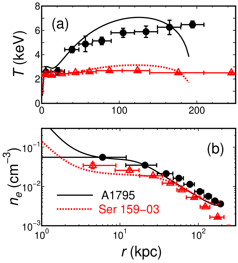
Figure 1: (a) Modeled temperature and (b) density profiles for A1795 (solid lines) and Ser 159–03 (dotted lines). Filled dots and empty triangles are the Chandra data for A1795 and Ser 159–03, respectively.

Figure 1 shows the model fits for the two clusters. The boundary conditions are presented in Table 2. The temperature $T(r_{i})$ is especially required to be fine-tuned for the fit. We use the Chandra data of A1795 obtained by Ettori et al. (2002) and the XMM-Newton data of Ser 159–03 obtained by Kaastra et al. (2001). The XMM-Newton data of A1795 are also obtained by Tamura et al. (2001) and they are similar to those obtained by Ettori et al. (2002), although the former is not deprojected contrary to the latter. The good agreement between the model and the data suggests that wave heating is a promising candidate of the mechanism that solves the cooling flow problem. In Figure 1, densities go to infinity and temperatures go down to zero at $r\sim 200$ kpc. This suggests that waves injected outside of this radius cannot reach the cluster center.

In Figure 2a, we present the wave velocity amplitude normalized by the sound velocity ($\alpha_{w}$). As the N-waves propagate into the central regions of the cluster, $\alpha_{w}$ increases rapidly. This is mainly because of the geometrical convergence to the cluster center, whereas the total wave luminosity (= energy flux times $r^{2}$) mostly dissipates through the inward propagation in itself. Since $\alpha_{w}>1$ at $r\lesssim 4$ kpc for both A1795 and Ser 159–03, the results may not be quantitatively correct there. We note that the gas velocity for the region of $r\gtrsim 4$ kpc is very small compared with the sound velocity and thus our ignorance of $vdv/dr$ in equation (2) is justified.

In Figure 2b, the ratio $F_{w}f_{c}/F_{c}$ is presented. The gaps at $\sim 10$ kpc reflect $F_{c}<0$. Assume that an observer made observations of the model clusters and the temperature distributions were exactly measured. If the observer assumed the classical conductivity, the heat flux measured by the observer should be $F_{c}/f_{c}$ ($f_{c}<1$) because of the definition of $F_{c}$ (equation [5]). Figure 2b shows that the observer would measure an X-ray emission much larger than that predicted by the classical thermal conduction ($F_{w}f_{c}/F_{c}>1$) if the energy swallowed by the black hole at the cluster center is small. Such large X-ray emissions have actually been estimated in some clusters (Voigt et al., 2002). Wave heating model can account for the observations without the help of heating by AGNs.

3 One-Dimensional Numerical Simulations

3.1 Models

In order to be compared with the results in the previous section, we performed one-dimensional numerical simulations. We solve the following equations:

$$\frac{\partial\rho}{\partial t}+\frac{1}{r^{2}}\frac{\partial}{\partial r}(r^{2}\rho v)=0\;,$$ (11)

$$\frac{\partial(\rho v)}{\partial t}+\frac{1}{r^{2}}\frac{\partial}{\partial r}(r^{2}\rho v^{2})=-\rho\frac{GM(r)}{r^{2}}-\frac{\partial p}{\partial r}\;,$$ (12)

$$\frac{\partial e}{\partial t}+\frac{1}{r^{2}}[r^{2}v(p+e)]=\frac{1}{r^{2}}\frac{\partial}{\partial r}\left[r^{2}\kappa(T)\frac{\partial T}{\partial r}\right]-n_{e}^{2}\Lambda(T)-\rho u\frac{GM(r)}{r^{2}}\;,$$ (13)

where the total energy is defined as $e=p/(\gamma-1)+\rho v^{2}/2$, and $\kappa(T)=\kappa_{0}T^{5/2}$. We ignore the self-gravity of ICM. For numerical simulations, we adopt the cooling function based on the detailed calculations by Sutherland & Dopita (1993),

$$n_{e}^{2}\Lambda=[C_{1}(k_{B})^{\alpha}+C_{2}(k_{B}T)^{\beta}+C_{3}]n_{i}n_{e}\>,$$ (14)

where $n_{i}$ is the ion number density and the units for $k_{B}T$ are keV. For an average metallicity $Z=0.3\>Z_{\sun}$ the constants in equation (14) are $\alpha=-1.7$, $\beta=0.5$, $C_{1}=8.6\times 10^{-3}$, $C_{2}=5.8\times 10^{-2}$, and $C_{3}=6.4\times 10^{-2}$, and we can approximate $n_{i}n_{e}=0.704(\rho/m_{H})^{2}$. The units of $\Lambda$ are $10^{-22}\>\rm ergs\>cm^{3}$ (Ruszkowski & Begelman, 2002). Note that equation (13) does not include the energy dissipation term contrary to equation (4). This is because the energy dissipation at shocks is included automatically in numerical simulations if shocks are resolved.

The hydrodynamic part of the equations is solved by a second-order advection upstream splitting method (AUSM) based on Liou & Steffen (1993, see also ). We use 500 unequally spaced meshes in the radial coordinate to cover a region with a radius of 300 kpc. The inner boundary is set at $r=1$ kpc. The innermost mesh has a width of $\sim 15$ pc, and the width of the outermost mesh is $\sim 3$ kpc. The following boundary conditions are adopted:

1. Variables except velocity have zero gradients at the center.

2. The inner edge is assumed to be a perfectly reflecting point.

3. The density and pressure at the outermost mesh are equal to specified values.

Waves are injected at the outermost mesh as

$$v(t)=\alpha_{w0}c_{s0}\sin\left(\frac{2\pi c_{s0}t}{\lambda_{0}}\right)\>,$$ (15)

where $\alpha_{w0}$ is the parameter.

3.2 Numerical Results

The mass distribution we assumed is the same as that of A1795 in Table 1 except for $T_{\rm av}$. We assume that the ICM is isothermal and in pressure equilibrium at $t=0$. For the NFW profile (equation [9]), the gas initial density profile is written as

$$\rho(r)=\rho_{0}\exp[-Bf(r/r_{s})]\;,$$ (16)

where

$$B=\frac{1}{m(1)}\frac{G\mu m_{H}M(r_{s})}{r_{s}k_{B}T_{\rm av}}\;,$$ (17)

$$m(x)=\ln(1+x)-\frac{x}{1+x}\;,$$ (18)

$$f(x)=1-\frac{1}{x}\ln(1+x)\;$$ (19)

(Suto, Sasaki, & Makino, 1998). The initial ICM temperature is $T_{\rm av}$. The density and pressure of the outer boundary are fixed at the initial values. We finish the calculations when the temperature of some of the meshes becomes zero because we do not treat mass dropout from the hot ICM. We define the time as $t_{\rm cool}$. If the temperature does not go to zero, we finish the calculations at $t=7$ Gyr. In this section, we set $n_{e}(0)=0.017\rm\>cm^{-3}$, $T_{\rm av}=7$ keV, and $\lambda_{0}=100$ kpc. Other model parameters are shown in Table 3.

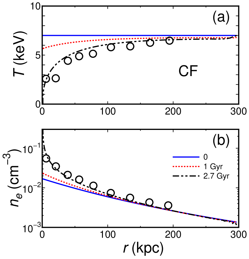
Figure 3: (a) Temperature and (b) density profiles for Model CF. Open circles are the Chandra data for A1795 (Ettori et al., 2002).

Figures 3 and 4 show the temperature and density profiles for Models CF and CO, respectively. For reference, the data of A1795 are shown (Ettori et al., 2002), although the detailed comparison is premature. Contrary to Figure 1, we use a linear scale for the distance from the cluster center for both temperature and density profiles to see shock structures. Model CF is a genuine cooling flow model; the temperature goes to zero at the cluster center at $t_{\rm cool}=2.7$ Gyr. In Model CO, conduction dominates cooling and the solution is stable for a long time. The suppression factor of the conductivity, $f_{c}=0.2$, in Model CO is the same as that of Zakamska & Narayan (2003). The temperature gradient at the cluster center is less steep than that obtained by Zakamska & Narayan (2003). This may be because of the differences of the boundary conditions or the initial conditions.

Figures 5 and 6 show the temperature and density profiles for Models W1 and W2, respectively. As we predicted in Figure 2, waves are amplified in the central region. A shock is seen at $r=13$ kpc in Model W1. Both temperature and density diverge at the cluster center because these are one-dimensional simulations and waves focus on the cluster center. In the outer region, the shape of waves is complicated. This is because we adopted the reflection condition at the inner boundary and the inward and outward waves interact. For Model W1, $t_{\rm cool}=4.7$ Gyr, and for Model W2, $t_{\rm cool}>7$ Gyr. They are much larger than $t_{\rm cool}$ for Model CF. This means the wave heating is effective.

In Models M1 and M2, we include both thermal conduction and waves. The results of Model M1 and Model M2 are almost the same as those of Model W1 and CO, respectively. The cooling time-scale $t_{\rm cool}$ of Model M1 is shorter than that of Model W1, because shocks are weakened by the thermal conduction. In model M2, the conduction dominates the wave heating.

4 Discussion

Our analytical model and numerical simulations show that acoustic waves are amplified at the cluster center and can heat the cluster core. One should note that our assumption, that is, the spherical symmetry, could affect the amplification quantitatively. For more realistic modeling, we should consider that real clusters are not exactly spherically symmetric. However, Pringle (1989) indicated that even if a cluster is not spherically symmetric, the lower temperature and smaller sound velocity at the cluster center should have waves focus on the center. In order to study this effect, we need to perform high-resolution multi-dimensional numerical simulations (Wada, Fujita, &, Suzuki 2003, in preparation). Since the focusing effect depends on the temperature gradient, it may solve the fine-tuning problem of the heating of cluster cores. If the cooling dominates heating, the temperature at the cluster center decreases and the temperature gradient in the core increases. This strengthens the focusing effect and wave heating becomes more efficient. Multi-dimensional simulations have another benefit; it is free from the inner boundary conditions that we set in our one-dimensional simulations.

If waves are actually responsible for the heating in cluster cores, weak shocks should be observed there in some clusters. In our simulations, waves are amplified at $r\lesssim 10-50$ kpc (Figures 5 and 6). Thus, if the wave length is large ($\gtrsim 100$ kpc), the shocks are not necessarily observed in all clusters. However, as pointed out by Churazov et al. (2003), the passing of waves may cause gas-sloshing around cluster cores. Observations of fine structures in many cluster cores will be useful to understand the heating mechanism there.

In the central regions of clusters, turbulence generated by interaction of amplified waves from various directions could be observed as broadened metal lines by future X-ray observatories. Observational studies of optical emission lines revealed that there is warm gas at some cluster centers and that the velocity widths range from 100 to $1000\rm\>km\>s^{-1}$ (Hu, Cowie, & Wang, 1985; Johnstone, Fabian, & Nulsen, 1987; Heckman et al., 1989). These warm gas may be embodied in and move with the hot turbulent ICM (see Loewenstein & Fabian, 1990).

5 Conclusions

Through analytical and numerical approaches, we have shown that acoustic waves generated by turbulence in the ICM in the outer region of a cluster can effectively heat the central part of the cluster. The heat flux by the waves may exceed that by thermal conduction. The process presented here is phenomenologically analogous to the collapse of a ”tsunami” (a seismic sea wave) at seashore owing to the change of depth of the sea. As in tsunamis, even if the waves have small amplitude at their origin, they could bring huge damage at a distant point, namely the cluster center. Of course, one should note that tsunamis are gravity-driven waves and not acousitc waves. In the analytical studies, we have obtained time-independent solutions and compared the predicted density and temperature profiles with the observed ones; they are consistent with each other. In general, we have confirmed the results obtained by the analytical studies by one-dimensional numerical simulations. Since we assumed that a cluster is spherically symmetric and the assumption leads to artificial focusing of waves, one should take the quantitative results with care. However, it has been indicated that even if a cluster is not spherically symmetric, waves are focused by the temperature gradient at the cluster center. Thus, it is worthwhile to study the wave heating by multi-dimensional analyses.

Table 1: Cluster Parameters

Cluster	$M_{\rm vir}$	$T_{\rm av}$	$r_{s}$	$c$
	($10^{14}\>M_{\sun}$)	(keV)	(Mpc)
A1795	12	7.5	0.46	4.2
Ser 159–03	2.6	2.7	0.31	4.7

Table 2: Model Parameters

Cluster	$f_{c}$	$\dot{M}$	$\lambda_{0}$	$\alpha_{w}(r_{i})$	$n_{e}(r_{i})$	$T(r_{i})$
		($M_{\sun}\rm\>yr^{-1}$)	(kpc)		($\rm cm^{-3}$)	(keV)
A1795	$2\times 10^{-3}$	50	100	3	0.5	0.6213
Ser 159–03	0.2	30	70	3	0.14	0.780

Table 3: Model Parameters

Model	$\alpha_{w0}$	$f_{c}$	$t_{\rm cool}$ (Gyr)
CF	0	0	2.7
CO	0	0.2	$\cdots$
W1	0.1	0	4.7
W2	0.2	0	$\cdots$
M1	0.1	0.002	4.3
M2	0.1	0.2	$\cdots$

Note. — No data for $t_{\rm cool}$ mean $t_{\rm cool}>7$ Gyr.

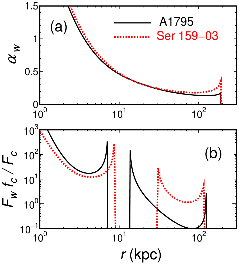
Figure 2: (a) Wave amplitudes and (b) the ratio of heat flux by waves to that by thermal conduction for A1795 (solid lines) and Ser 159–03 (dotted lines).

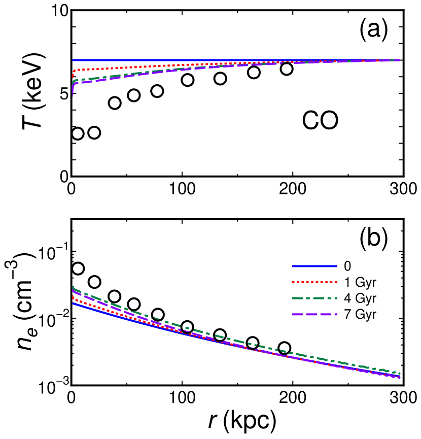
Figure 4: The same as Figure 3 but for Model CO

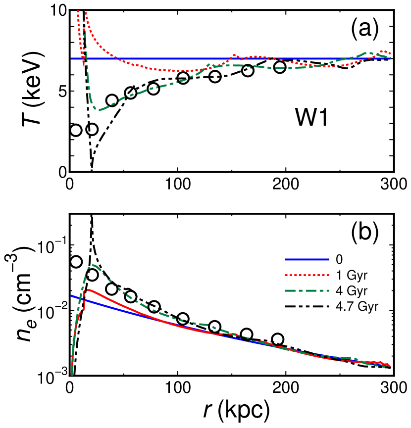
Figure 5: The same as Figure 3 but for Model W1

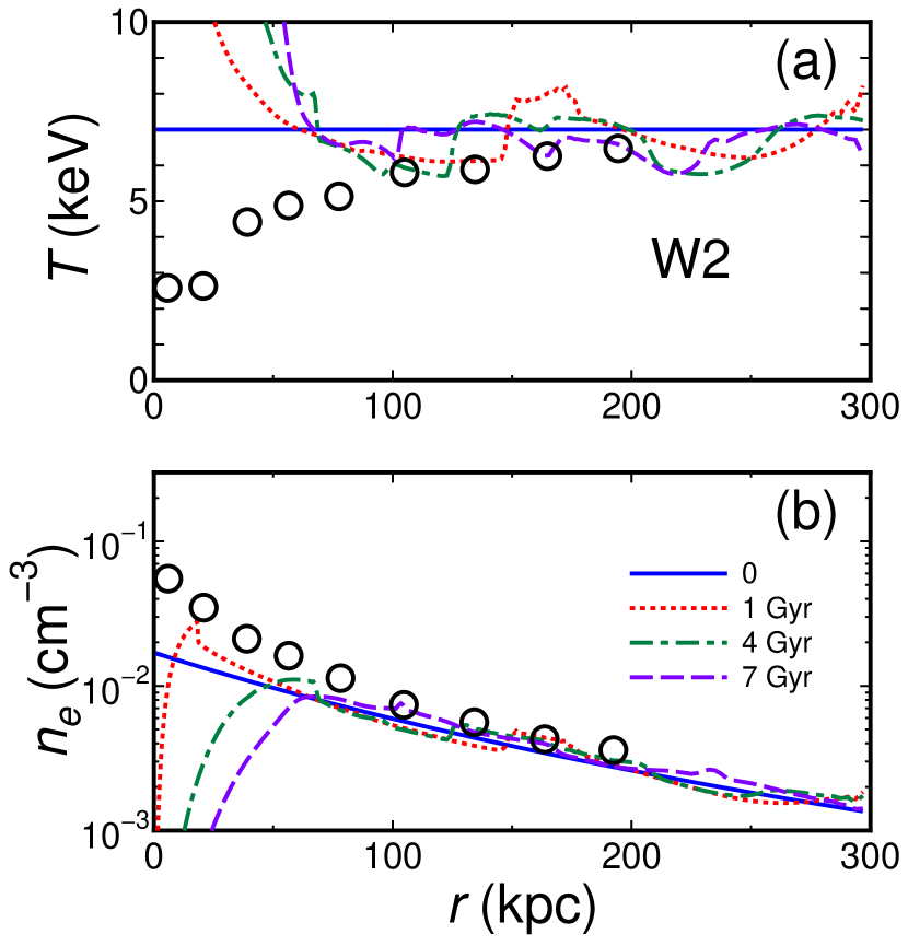
Figure 6: The same as Figure 3 but for Model W2

References

- Allen & Fabian (1997) Allen, S. W., & Fabian, A. C. 1997, MNRAS, 286, 583
- Basson & Alexander (2003) Basson, J. F. & Alexander, P. 2003, MNRAS, 339, 353
- Binney & Tabor (1995) Binney, J., & Tabor, G. 1995, MNRAS, 276, 663
- Blanton et al. (2003) Blanton, E. L., Sarazin, C. L., & McNamara, B. R. 2003, ApJ, 585, 227
- Blanton et al. (2001) Blanton, E. L., Sarazin, C. L., McNamara, B. R., & Wise, M. W. 2001, ApJ, 558, L15
- Böhringer & Fabian (1989) Böhringer, H. & Fabian, A. C. 1989, MNRAS, 237, 1147
- Böhringer & Hensler (1989) Böhringer, H., & Hensler, G. 1989, A&A, 215, 147
- Böhringer et al. (2002) Böhringer, H., Matsushita, K., Churazov, E., Ikebe, Y., & Chen, Y. 2002, A&A, 382, 804
- Böhringer & Morfill (1988) Böhringer, H., & Morfill, G. E. 1988, ApJ, 330, 609
- Böhringer et al. (1993) Böhringer, H., Voges, W., Fabian, A. C., Edge, A. C., & Neumann, D. M. 1993, MNRAS, 264, L25
- Bregman & David (1988) Bregman, J. N., & David, L. P. 1988, ApJ, 326, 639
- Brighenti & Mathews (2003) Brighenti, F., & Mathews, W. G. 2003, ApJ, 587, 580
- Brüggen & Kaiser (2002) Brüggen, M. & Kaiser, C. R. 2002, Nature, 418, 301
- Bryan & Norman (1998) Bryan, G. L., & Norman, M. L. 1998, ApJ, 495, 80
- Ciotti & Ostriker (2001) Ciotti, L., & Ostriker, J. P. 2001, ApJ, 551, 131
- Churazov et al. (2001) Churazov, E., Brüggen, M., Kaiser, C. R., Böhringer, H., & Forman, W. 2001, ApJ, 554, 261
- Churazov et al. (2002) Churazov, E., Sunyaev, R., Forman, W., & Böhringer, H. 2002, MNRAS, 332, 729
- Churazov et al. (2003) Churazov, E., Forman, W., Jones, C., & Böhringer, H. 2003, ApJ, 590, 225
- Edge et al. (1992) Edge, A. C., Stewart, G. C., & Fabian, A. C. 1992, MNRAS, 258, 177
- Ettori et al. (2002) Ettori, S., Fabian, A. C., Allen, S. W., & Johnstone, R. M. 2002, MNRAS, 331, 635
- Fabian (1994) Fabian, A. C. 1994, ARA&A, 32, 277
- Fabian et al. (2000) Fabian, A. C. et al. 2000, MNRAS, 318, L65
- Fabian et al. (2002) Fabian, A. C., Voigt, L. M., & Morris, R. G. 2002, MNRAS, 335, L71
- Friaca (1986) Friaca, A. C. S. 1986, A&A, 164, 6
- Fujita et al. (2002) Fujita, Y., Sarazin, C. L., Kempner, J. C., Rudnick, L., Slee, O. B., Roy, A. L., Andernach, H., & Ehle, M. 2002, ApJ, 575, 764
- Gaetz (1989) Gaetz, T. J. 1989, ApJ, 345, 666
- Heckman et al. (1989) Heckman, T. M., Baum, S. A., van Breugel, W. J. M., & McCarthy, P. 1989, ApJ, 338, 48
- Hu et al. (1985) Hu, E. M., Cowie, L. L., & Wang, Z. 1985, ApJS, 59, 447
- Huang & Sarazin (1998) Huang, Z., & Sarazin, C. L. 1998, ApJ, 496, 728
- Ikebe et al. (1997) Ikebe, Y. et al. 1997, ApJ, 481, 660
- Johnstone et al. (2002) Johnstone, R. M., Allen, S. W., Fabian, A. C., & Sanders, J. S. 2002, MNRAS, 336, 299
- Johnstone et al. (1987) Johnstone, R. M., Fabian, A. C., & Nulsen, P. E. J. 1987, MNRAS, 224, 75
- Kaastra et al. (2001) Kaastra, J. S., Ferrigno, C., Tamura, T., Paerels, F. B. S., Peterson, J. R., & Mittaz, J. P. D. 2001, A&A, 365, L99
- Kaiser & Binney (2003) Kaiser, C. R., & Binney, J. 2003, MNRAS, 338, 837
- Kempner et al. (2002) Kempner, J. C., Sarazin, C. L., & Ricker, P. M. 2002, ApJ, 579, 236
- Liou & Steffen (1993) Liou, M., & Steffen, C. 1993, J. Comp. Phys., 107, 23
- Loewenstein & Fabian (1990) Loewenstein, M., & Fabian, A. C. 1990, MNRAS, 242, 120
- Makishima et al. (2001) Makishima, K. et al. 2001, PASJ, 53, 401
- Matsushita et al. (2002) Matsushita, K., Belsole, E., Finoguenov, A., & Böhringer, H. 2002, A&A, 386, 77
- Mazzotta et al. (2002) Mazzotta, P., Kaastra, J. S., Paerels, F. B., Ferrigno, C., Colafrancesco, S., Mewe, R., & Forman, W. R. 2002, ApJ, 567, L37
- McNamara et al. (2000) McNamara, B. R. et al. 2000, ApJ, 534, L135
- McNamara et al. (2001) McNamara, B. R. et al. 2001, ApJ, 562, L149
- McWhirter et al. (1975) McWhirter, R. W. P., Thonemann, P. C., & Wilson, R. 1975, A&A, 40, 63
- Nagai et al. (2003) Nagai, D., Kravtsov, A. V., & Kosowsky, A. 2003, ApJ, 587, 524
- Narayan & Medvedev (2001) Narayan, R. & Medvedev, M. V. 2001, ApJ, 562, L129
- Navarro et al. (1997) Navarro, J. F., Frenk, C. S., & White, S. D. M. 1997, ApJ, 490, 493
- Osterbrock (1961) Osterbrock, D. E. 1961, ApJ, 134, 347
- Peres et al. (1998) Peres, C. B., Fabian, A. C., Edge, A. C., Allen, S. W., Johnstone, R. M., & White, D. A. 1998, MNRAS, 298, 416
- Peterson et al. (2001) Peterson, J. R. et al. 2001, A&A, 365, L104
- Pringle (1989) Pringle, J. E. 1989, MNRAS, 239, 479
- Quilis et al. (2001) Quilis, V., Bower, R. G., & Balogh, M. L. 2001, MNRAS, 328, 1091
- Rephaeli (1987) Rephaeli, Y. 1987, MNRAS, 225, 851
- Reynolds et al. (2002) Reynolds, C. S., Heinz, S., & Begelman, M. C. 2002, MNRAS, 332, 271
- Roettiger et al. (1999) Roettiger, K., Stone, J. M., & Burns, J. O. 1999, ApJ, 518, 594
- Ruszkowski & Begelman (2002) Ruszkowski, M. & Begelman, M. C. 2002, ApJ, 581, 223
- Saito & Shigeyama (1999) Saito, R., & Shigeyama, T. 1999, ApJ, 519, 48
- Sarazin (1986) Sarazin, C. L. 1986, Rev. Mod. Phys., 58, 1
- Saxton et al. (2001) Saxton, C. J., Sutherland, R. S., & Bicknell, G. V. 2001, ApJ, 563, 103
- Soker (2003) Soker, N. 2003, MNRAS, 342, 463
- Soker et al. (2002) Soker, N., Blanton, E. L., & Sarazin, C. L. 2002, ApJ, 573, 533
- Soker et al. (2001) Soker, N., White, R. E., David, L. P., & McNamara, B. R. 2001, ApJ, 549,
- Sparks (1992) Sparks, W. B. 1992, ApJ, 399, 66
- Stein & Schwartz (1972) Stein, R. F. & Schwartz, R. A. 1972, ApJ, 177, 807
- Sutherland & Dopita (1993) Sutherland, R. S. & Dopita, M. A. 1993, ApJS, 88, 253
- Suto et al. (1998) Suto, Y., Sasaki, S., & Makino, N. 1998, ApJ, 509, 544
- Suzuki (2002) Suzuki, T. K. 2002, ApJ, 578, 598
- Takahara & Takahara (1979) Takahara, M., & Takahara, F. 1979, Prog. Theor. Phys., 62, 1253
- Takahara & Takahara (1981) Takahara, M., & Takahara, F. 1981, Prog. Theor. Phys., 65, L369
- Tucker & Rosner (1983) Tucker, W. H. & Rosner, R. 1983, ApJ, 267, 547
- Tamura et al. (2001) Tamura, T. et al. 2001, A&A, 365, L87
- Ulmschneider (1971) Ulmschneider, P. 1971, A&A, 12, 297
- Voigt et al. (2002) Voigt, L. M., Schmidt, R. W., Fabian, A. C., Allen, S. W., & Johnstone, R. M. 2002, MNRAS, 335, L7
- Wada & Norman (2001) Wada, K. & Norman, C. A. 2001, ApJ, 547, 172
- White et al. (1997) White, D. A., Jones, C., & Forman, W. 1997, MNRAS, 292, 419
- Zakamska & Narayan (2003) Zakamska, N. L., & Narayan, R. 2003, ApJ, 582, 162