Molecular gas in the galaxy M 83

We present ¹²CO $J$=1–0 and $J$=2–1 Swedish-ESO Submillimetre Telescope (SEST) observations of the barred spiral galaxy M83 (NGC5236). The size of the CO maps is 10′$\times$10′ and they cover the entire optical disk. The grid spacing is 11″ for CO($J$=1–0) and 11″ or 7″ for CO($J$=2–1) depending on the position in the galaxy. In total we have obtained spectra in 1900 and 2574 positions in the CO($J$=1–0) and CO($J$=2–1) lines, respectively. The CO emission is strongly peaked toward the nucleus, which breaks up into two separate components in the CO($J$=2–1) data due to the higher spatial resolution. Emission from the bar is strong, in particular on the leading edges of the bar. The molecular gas arms are clearly resolved and can be traced for more than 360°. Emission in the inter-arm regions is detected. The average CO ($J$=2–1)/($J$=1–0) line ratio is 0.77. The ratio is lower than this on the spiral arms and higher in the inter-arm regions. The arms show regularly spaced concentrations of molecular gas, Giant Molecular Associations (GMA’s), whose masses are of the order 10⁷ M_⊙. The total molecular gas mass is estimated to be 3.9$\times$10⁹ M_⊙. This mass is comparable to the total HI mass, but H₂ dominates in the optical disk. In the disk, H₂ and HI show very similar distributions, including small scale clumping. We compare the molecular gas distribution with those of other star formation tracers, such as B and H$\alpha$ images.

1 Introduction

In disk galaxies the mass of the molecular (H₂) gas is usually similar to, or a bit less than, that of the atomic (HI) gas (Young & Scoville, 1991; Casoli et al., 1998). However, their spatial distributions are completely different, both in the radial and in the vertical directions. The molecular gas is concentrated to a relatively thin disk, which often has a radial extent similar to that of the optical disk and a vertical scale height which is smaller than that of the young, massive stars. The radius of the HI disk is usually much larger than that of the optical disk (up to 5 times the Holmberg radius), and the atomic gas is also less concentrated to the disk in the vertical direction (Knapp, 1987).

If the mass surface density in a region exceeds a certain critical density, massive star formation is triggered (Kennicutt, 1989). So, naturally, the study of interstellar gas, and especially the molecular gas phase, plays a key role in understanding the structure and evolution of galaxies. Unfortunately, direct studies (in emission) of the cold ($\sim$10 K) H₂ gas in molecular clouds are very difficult, since the energy of the first excited rotational level is of the order of 500 K (corresponding to a wavelength of 28 $\mu$m), and therefore much larger than the average kinetic temperatures in the clouds. Carbon monoxide (CO) is the second most common molecule with a relative abundance with respect to H₂ of about 10^-4. The heavy, asymmetrical CO molecule has rotational levels which are easily excited by collisions with H₂, and it radiates at mm wavelengths where observations can be carried out using radio telescopes. However, the conversion factor which is used to derive the H₂ column density from the velocity-integrated CO intensity, $X_{\rm CO}$, is not well-known, and this is a source of major uncertainty (Young & Scoville, 1991; Combes, 1991).

CO emission at mm wavelengths has been detected in many galaxies ranging in distance from the nearby irregular galaxies The Large and The Small Magellanic Clouds to quasars at a redshift of more than $z$ $\sim$ 5, and in essentially all galaxy types. A large survey of 300 galaxies (of which 236 were detected) of different types was done by Young et al. (1995) using the FCRAO 14 m telescope. The analysis of the data is still ongoing, but some interesting results have been published, e.g., the conversion factor ($X_{\rm CO}$) appears relatively constant, at least within each galaxy type (Young & Rownd, 2001), and the global star formation efficiency decreases with increasing galaxy size (Young, 1999). In this survey a number of galaxies were also mapped and radial distributions of the molecular gas can be examined. Recently, in a more detailed study, 28 nearby galaxies were mapped with the 45 m Nobeyama telescope (Kuno et al., 2000; Nishiyama et al., 2001). Among other things, this showed that barred and non-barred galaxies differ in both the distribution and the kinematics of the molecular gas. Another large survey is the BIMA SONG project (Regan et al., 2001; Helfer et al., 2003), in which 44 nearby ($v_{\sun}<2000$ km s^-1) galaxies have been observed with the BIMA array and the NRAO 12m telescope. Early results show that many galaxies have multiple peaks at the nucleus, that the CO distribution usually cannot be fitted with a single exponential disk model, and that the ratio of the scale length in the CO disk and the scale length in the stellar disk is on average 1 (but the scatter around this average is large).

Detailed morphological studies of selected galaxies are more rare, partly because there are so few nearby galaxies for which the limited angular resolution of radio telescopes gives an adequate spatial resolution. Nakai et al. (1994) outlined a number of important observational conditions that should be fulfilled in order to be able to extract useful information on the properties of the molecular gas in different regions of a galaxy: (1) a spatial resolution better than one kpc, which is the typical width of molecular spiral arms and the spacing between them, (2) high sensitivity in order to detect the weak inter-arm emission, (3) mapping of a large field in order to get statistically meaningful results, and (4) filled aperture telescope data, since it is important to detect the diffuse emission in the inter-arm regions. To this list we add a fifth condition, (5) the observation should be carried out in (at least) two lines per molecular species (and preferably also partially observed in a few isotopomers) in order to gain insight into the density, temperature, and chemistry of the molecular gas.

Single-dish measurements are therefore essential to our determination of the molecular gas distribution, its relation to star formation activity, its location with respect to dynamical resonances, and the total reservoir of gas capable of forming future generations of stars. The most detailed single-dish maps of molecular gas in spiral galaxies are the mappings of M 51, using the IRAM 30m telescope (Garcia-Burillo et al., 1993) and the Nobeyama 45m telescope (Nakai et al., 1994), and two projects currently underway to map our neighbor M 31 (Loinard et al., 1999; Nieten et al., 2000). In M 51 the molecular spiral arms were resolved, and streaming motions were detected. Also, the CO emission was found to peak on the inside of the spiral arms, giving support to a scenario where molecular gas agglomerates and forms new stars, which in their turn produce H$\alpha$ emission and other star formation tracers, close to the spiral arms. Support was also found for the proposal that gravitational instability in the disk is the main formation mechanism of GMAs (Galactic Molecular Associations of mass $\sim$10⁷ M_⊙). Other large spiral galaxies that have been completely surveyed in CO with a single-dish telescope are IC 342 (Crosthwaite et al., 2001), M 101 (Kenney et al., 1991), NGC 253 (Houghton et al., 1997), and NGC 6946 (Tacconi & Young, 1989). Some large scale CO mapping projects, such as the OVRO maps of M 51 (Aalto et al., 1999) and M 83 (Rand et al., 1999), have been done using mm-wave interferometers. Although this gives a superior angular resolution and important unique information, a significant part of the emission is resolved out (especially the diffuse component in the inter-arm regions).

We have mapped the CO($J$=1–0) and CO($J$=2–1)  emission in the barred, grand-design, spiral galaxy M 83 located at a distance of 4.5 Mpc. The observations were done with the 15 m Swedish-ESO Submillimetre Telescope (SEST) providing beam widths of 45″ (1–0) and 23″ (2–1), which corresponds to 980 pc and 500 pc, respectively, at the adopted distance. M 83 is among the brightest galaxies in terms of CO emission, and it is also one of the most nearby barred spirals. Its low inclination ($\approx$24^∘) and proximity make it a perfect candidate to investigate the correlation between various tracers of stellar activity.

In this paper we present the CO($J$=1–0) and CO($J$=2–1) observational data. We show the distribution of the molecular gas, as inferred from the CO data, and compare it to the distributions of optical light, obtained in different filters, and the HI gas. We examine the CO ($J=2-1$)/($J=1-0$) line ratio and its variation over the disk. In two forth-coming papers we will present and discuss the kinematics of the molecular gas, and discuss the relation between the molecular gas and star formation.

2 The galaxy M83

M 83 is a relatively nearby, barred, grand-design, spiral galaxy (see Table 1). It is viewed almost face-on and the bar is aligned with the major axis. Color images show clumpy, well-defined spiral arms, evidently rich in young blue stars. It is also fairly symmetrical and has no nearby massive optical companions and no immediate evidence of interaction or outflows.

Table 1: General Parameters of M 83.

Morphological Typea	SAB(s)c
IR center:b
R.A. (J2000)	$13^{\rm h}37^{\rm m}00\aas@@fstack{s}8$
Decl. (J2000)	$-29\degr 51\arcmin 56\arcsec$
LSR systemic velocity (opt)c	506 km s-1
Distanced	4.5 Mpc
Position anglec	45°
Inclinationf	24°
Holmberg diameter (D0)e	14$\aas@@fstack{\prime}$6
$M_{\rm HI}$e	7.7$\times 10^{9}\leavevmode\nobreak\ {\rm M}_{\odot}$
$M_{{\rm H}_{2}}$g	3.9$\times 10^{9}\leavevmode\nobreak\ {\rm M}_{\odot}$
a de Vaucouleurs et al. (1976); b Sofue & Wakamatsu (1994); c Comte (1981); d Thim et al. (2003); e Huchtmeier & Bohnenstengel (1981); f Talbot et al. (1979); g this paper

Due to its favorable properties it is one of the most well-observed galaxies: HI (Rogstad et al., 1974; Huchtmeier & Bohnenstengel, 1981; Tilanus & Allen, 1993), radio continuum (Ondrechen, 1985; Neininger et al., 1993), CO (see Table 2), IR continuum (Adamson et al., 1987; Fitt et al., 1992; Elmegreen et al., 1998), optical continuum (Jensen et al., 1981), Balmer lines (Comte, 1981; de Vaucouleurs et al., 1983; Tilanus & Allen, 1993), and in X-ray emission (Immler et al., 1999; Soria & Wu, 2002).

Table 2: Previous CO observations of M 83 divided into two groups: single-dish and interferometer observations. If no location is given, the map is centered on the nucleus and oriented along the major axis.

Reference	Transition	Beam and Telescope	Map description
Combes et al. (1978)	CO(1-0)	64″, NRAO 11m	10 positions, 6′$\times$3′
Lord (1987)	CO(1-0)	45″, FCRAO 14m	21 positions, 5′$\times$5′
Wiklind et al. (1990)	CO(1-0)	45″, SEST 15m	196 positions, SE quadrant, 3′$\times$2′
	CO(2-1)	23″, SEST 15m	143 positions, SE quadrant, 1$\aas@@fstack{\prime}$5$\times$1$\aas@@fstack{\prime}$5
Handa et al. (1990)	CO(1-0)	16″, NRO 45m	85 positions, 3$\aas@@fstack{\prime}$5$\times$1′
Wall (1991)	CO(2-1)	22″, JCMT 15m	43 positions
	CO(3-2)	22″, CSO 10m	8 positions
Petitpas & Wilson (1998)	CO(3-2)	14″, JCMT 15m	81 positions, 0$\aas@@fstack{\prime}$7$\times$0$\aas@@fstack{\prime}$7
	CO(4-3)	12″, JCMT 15m	46 positions, 0$\aas@@fstack{\prime}$7$\times$0$\aas@@fstack{\prime}$5
Israel & Baas (2001)	CO(2-1)	21″, JCMT 15m	49 positions, 1$\aas@@fstack{\prime}$2$\times$2$\aas@@fstack{\prime}$0
	CO(3-2)	14″, JCMT 15m	55 positions, 1$\aas@@fstack{\prime}$2$\times$1$\aas@@fstack{\prime}$7
	CO(4-3)	11″, JCMT 15m	20 positions, 0$\aas@@fstack{\prime}$5$\times$0$\aas@@fstack{\prime}$5
Crosthwaite et al. (2002)	CO(1-0)	55″, NRAO 12m	On-the-fly, 10′$\times$10′
	CO(2-1)	28″, NRAO 12m	On-the-fly, 8′$\times$8′
Thuma et al. (in prep.)	CO(3-2)	23″, SMT 10m	374 positions, 5$\aas@@fstack{\prime}$5$\times$2$\aas@@fstack{\prime}$5
	CO(4-3)	17″, SMT 10m	21 positions
This paper	CO(1-0)	45″, SEST 15m	1900 positions, 10′$\times$10′
	CO(2-1)	23″, SEST 15m	2574 positions, 10′$\times$10′
Lord & Kenney (1991)	CO(1-0)	12$\aas@@fstack{\prime\prime}$4$\times$5$\aas@@fstack{\prime\prime}$4, OVRO	Inner eastern arm, 1$\aas@@fstack{\prime}$5$\times$1$\aas@@fstack{\prime}$5
Kenney & Lord (1991)	CO(1-0)	8$\aas@@fstack{\prime\prime}$9$\times$5$\aas@@fstack{\prime\prime}$8, OVRO	Western bar end, 1$\aas@@fstack{\prime}$5$\times$1$\aas@@fstack{\prime}$5
Handa et al. (1994)	CO(1-0)	12″$\times$6″, NMA	Nucleus, 1$\aas@@fstack{\prime}$1$\times$1$\aas@@fstack{\prime}$1
Rand et al. (1999)	CO(1-0)	6$\aas@@fstack{\prime\prime}$5$\times$3$\aas@@fstack{\prime\prime}$5, OVRO	Inner eastern arm, 2$\aas@@fstack{\prime}$9$\times$1$\aas@@fstack{\prime}$1

The distance to M 83 is a long-standing issue. Sandage & Tammann (1974) used a relation between the luminosity class and the angular size of the three largest Hii regions to deduce a distance of 8.9 Mpc, while de Vaucouleurs (1979) used a number of methods to derive a distance of 3.7 Mpc. Recently, Cepheids have been observed in M 83 by Thim et al. (2003) using the VLT. Twelve Cepheid candidates were observed and the distance was estimated to be 4.5$\pm$0.3 Mpc. This distance is also supported by studies that seem to indicate that M 83 interacted with NGC 5253 some 1–2 $\times$ 10⁹ years ago (Kobulnicky & Skillman, 1995; Calzetti et al., 1999). This small, metal-poor dwarf galaxy about 2° SE of M 83 has roughly the same systemic velocity, and shows a highly disturbed HI velocity field and intense star formation. There has been a number of distance measurements to NGC 5253 (Saha et al., 1995; Parodi et al., 2000; Gibson et al., 2000), and they all favor a distance of about 4 Mpc.

3 Observations and data reduction

3.1 Observations

The CO($J=1-0$ and $J=2-1$) observations of M 83 were done using the 15 m SEST during two epochs, 1989-1994 and 1997-2001 [a description of the telescope is given by Booth et al. (1989)]. Between 1988 and 1994 we observed CO($J$=1–0) in the inner disk of M 83. A segment of these observations were presented in Wiklind et al. (1990). In 1998 and 1999 we completed this map by observing the outer disk. During the latter observations it was possible to do simultaneous observations in two frequency bands. We used this option to observe the CO($J$=2–1) line in parallel with the CO($J$=1–0) line. The map spacing (11″) and integration times were set by the requirements on the CO($J$=1–0) data. In 2000 and 2001 our primary task was to fill in the central area of the CO($J$=2–1) map. For these observations we chose a grid spacing of 7″. We used the other receiver to observe the ¹³CO($J$=1–0) line, but these data will be presented elsewhere.

The receivers were centered on the CO($J$=1–0) and CO($J$=2–1) lines (115.271 and 230.538 GHz, respectively), where the full half-power beam widths (HPBWs) are 45$\arcsec$ and 23$\arcsec$, respectively. Observations performed during 1988-1994 were made with a cooled Schottky-diode mixer receiver, while the subsequent observations were done with SIS receivers. All receivers operated in the single-sideband mode, and the average system temperatures, corrected for the atmospheric and antenna ohmic losses, were 660 K and 390 K for the CO($J$=1–0) observations in the first and second epoch, respectively, and 340 K for the CO($J$=2–1) observations. The backends were acousto-optical spectrometers, with channel separations of 0.69 MHz (1.8 and 0.9 km s^-1 at the two rest frequencies) and total bandwidths varying between 0.5 and 1 GHz.

We used the dual beam switching mode with a throw of $\approx$12$\arcmin$ in azimuth. In dual beam switching the source is placed first in the signal beam and then in the reference beam. The two spectra produced are then subtracted to generate a spectrum with a minimum of baseline variation. Great care was taken to ensure the quality of the data. No observations were done below the elevation of 30° or above 84° (M 83 passes within 1° from zenith at SEST), and pointing was regularly checked and updated using the SiO($v$=1, $J=2-1$) maser line of the nearby AGB-star W Hya ($\approx$3^∘ from M 83). Total pointing errors were typically less than 3″, and data with pointing offsets suspected to be larger than 4″ were disregarded in the subsequent data reduction (when possible, map points with such data were reobserved). The intensity scale was calibrated using the conventional chopper wheel method, and the internal calibration errors in the corrected antenna temperatures, $T_{\rm A}^{*}$, is within $\pm$10% according to the SEST manual. In this paper we use the main beam brightness temperature scale $T_{\rm mb}$, which is defined by $T_{\rm mb}\equiv T_{\rm A}^{*}/\eta_{\rm mb}$. According to the SEST manual the main beam efficiencies [$\eta_{\rm mb}$(115 GHz)=0.7, $\eta_{\rm mb}$(230 GHz)=0.5] have been constant throughout the period of our observations.

Table 3: SEST observation parameters for M 83.

	CO(J=1–0)	CO(J=2–1)
Center of the CO map	R.A. = $13^{\rm h}36^{\rm m}59\aas@@fstack{s}4$ (J2000)
	Decl.= $-29\degr 52\arcmin 05\arcsec$ (J2000)
Rest frequency	115.271204 GHz	230.53799 GHz
Beam size	45″	23″
Center velocity (LSR)	520 km s-1	520 km s-1
Average rms ($T_{\rm mb}$ scale)	74 mK	90 mK
Channel separation	$\leq$0.69 MHz	0.69 MHz
Number of channels	$\geq$700	1000
Main beam efficiency ($\eta_{\rm mb}$)	0.7	0.5
Aperture efficiency ($\eta_{\rm A}$)	0.58 (27 Jy/K)	0.38 (41 Jy/K)

The observations were centered on the coordinates $13^{\rm h}36^{\rm m}59\aas@@fstack{s}4$, $-29\degr 52\arcmin 05\arcsec$ (J2000), which is the optical center given by de Vaucouleurs et al. (1976). For CO($J$=1–0) we have 3634 spectra in 1900 positions with 11″ spacing, and the coverage is complete out to a radius of 4′20″. The grid extends parallel to the equatorial coordinate system, and the dense spacing (1/4 of the HPBW) was chosen in order to facilitate the use of deconvolution techniques. The integration time per position was chosen to render an rms around 70 mK ($T_{\rm mb}$-scale) at the original velocity resolution (1.8 km s^-1). During normal weather conditions we had a typical on-source integration time of 60 seconds. Among the final 1900 spectra we have $\geq$ 3$\sigma$ detections in 1201 positions, i.e. a detection rate of 63%. The average rms noise in our data set is 74 mK, which should be compared to the peak temperature which usually lies around 0.3 K ($T_{\rm mb}$-scale) in the spiral arms in the outskirts of the map.

In CO($J$=2–1) we have two maps with different spacings covering two, partly overlapping, regions. The inner 5′$\times$3′ is covered with a 7″ grid, while the rest of the optical disk (out to a radius of 4$\aas@@fstack{\prime}$5) is covered with an 11″ grid. In total, we have spectra in 2574 positions, out of which we have $\geq$ 3$\sigma$ detections in 1898 positions (73% detection rate). The spectra have an average rms of about 90 mK at the original velocity resolution (0.9 km s^-1). The observational parameters are summarized in Table 3.

3.2 Data reduction

The data reduction was carried out with class, drp, and xs. During the CO($J$=1–0) observations, the number of channels and the frequency resolution varied between the spectrometers. We therefore resampled all data to 1.8 km s^-1 (0.69 MHz) and by selecting the central 700 channels this gave us a (fully sufficient) total bandwidth of 1260 km s^-1.

After flagging bad channels, and replacing them with a value obtained from interpolation between adjacent channels, all spectra at the same position were averaged using a weight determined by the noise level. The baselines were stable, and only linear polynomial fits were subtracted. From the spectra we created a fits data cube for each transition, where the first two axes represent spatial coordinates, and the third axis represents frequency (or velocity).

We adopted a relatively dense grid spacing, compared to the beamwidth, in order to be able to increase the spatial resolution of the data using a mem-deconvolution routine (maximum entropy method); the Statistical Image Analysis (SIA) routine (Rydbeck, 2000). This procedure is particularly effective on a data set as densely spaced as ours (spacing in the range 1/4–1/2 of the HPBW), due to the high redundancy. The routine starts by deconvolving a velocity-integrated intensity map, where the velocity range is chosen to be large enough to encompass all the emission. Once this is done, the procedure splits the initial velocity range into three equally wide regions, calculates their velocity-integrated intensities, and then deconvolves these three maps, using the deconvolved map from the previous step as the input guess. The deconvolution continues in this hierarchical manner, successively narrowing the velocity interval, until a velocity range of 5 km s^-1 is reached. To deconvolve beyond this point is not meaningful since the S/N-ratios in the (narrow velocity range) maps drop below a critical value. For each of the two CO transitions we created 81 (3⁴) maps per transition (each covering about 5 km s^-1) which we assembled into a data cube per transition. By convolving the mem-deconvolved data cube by a Gaussian with a FWHM equal to the observational HPBW and comparing with the raw spectra, we verified that the mem-results are reliable, and that the raw data set is homogeneous, i.e., free from variations in gain and pointing errors. The angular resolutions of the mem-cubes are estimated to be $\approx$22″ and $\approx$14″ for the CO($J$=1–0) and CO($J$=2–1) data, respectively, and the velocity resolution is 5 km s^-1.

We have also constructed convolved data sets by convolving the raw data cubes with a HPBW beam size of 20$\arcsec$ and 15$\arcsec$ for the CO($J$=1–0) and CO($J$=2–1) data, respectively (the spacing in these cubes are 11″). Even if this degrades the resolution by $\approx$10–20%, the average rms noise in these cubes decreases from 74 mK to 25 mK and from 90 mK to 31 mK, respectively. The dramatically decreased noise level is due to the fact that the spacing is small with respect to the HPBW of the convolution kernels. Since the peak intensity in the spectra are relatively unaffected by this process, the average S/N-ratio in the spectra increases by a factor of $\approx$3. As a result of this, the detection rate increases to 92% and 89% for the CO($J$=1–0) and CO($J$=2–1) data, respectively (cf Sect. 3.1). These cubes were used to cross-check the results we got from the mem-deconvolved data. Some results were also derived directly from the convolved cubes, especially in cases where the velocity resolution was more important than the spatial resolution. Furthermore, we convolved the raw CO($J$=2–1) cube with a beam size of 44″ and regridded it to 11″ spacing in order to compare with the convolved CO($J$=1–0) cube at the same resolution ($\approx$49″).

In order to avoid problems with baseline irregularities when calculating the zero moment (over velocity) of the intensities we used a sliding window technique where at each position integration was performed inside a velocity window whose center and width depend on the position within the galaxy. We checked carefully that the window always covered all the emission.

3.3 Correction for the error beam

A closer inspection of the CO($J$=2–1) spectra reveals, apart from the expected main component seen in the CO($J$=1–0) spectra, a broad (velocity width 400 km s^-1) and faint (peak intensity around 0.03 K) component. Despite the low peak intensity of this feature, its integrated intensity is quite appreciable due to its large width. Typically, it makes up to 20%–35% of the total integrated intensity. This feature was discovered in the mem-deconvolved data, which are noise-free, but it can be seen also in spectra produced by convolving the raw CO($J$=2–1) data cube with a 45″ beam. The appearance of this broad component changed with position in the disk, and we found that its shape could, in any given position, be reproduced very well by convolving the data set with a relatively large Gaussian beam. This indicates that the SEST picks up emission from a much larger area than the HPBW of 23”, i.e., at 230 GHz the SEST suffers from a non-negligible error beam.

We have corrected the CO($J$=2–1) data sets for this error using a method described in Appendix A. We have found no trace of an error beam contribution in the CO($J$=1–0) data (not unexpectedly, considering the higher main beam efficiency), and consequently we have not applied any correction to these data.

4 The data

4.1 Spectra

In general, the spectra have a smooth and symmetric shape, but in some areas they show deviations. The spectra close to the nucleus are asymmetric, show extended wings, and a few of them have multiple peaks. The main reason for this is a large velocity gradient over spatial scales small compared to the telescope beam. Further out in the disk there are a few (interarm) regions which show multiple-peak spectra, such as the “Gould-belt structure” located about 3$\arcmin$ SE of the galaxy center (Comerón, 2001). However, in the vast majority of the observed positions the spectral feature can be well described by a single, Gaussian profile.

4.1.1 The CO($J$=1–0) spectra

In the arms we find that the peak temperatures are typically 0.2–0.4 K, and in the inter-arm regions they are about 0.1 K. The spectra are widest in the nuclear region with (Gaussian) widths of 80–100 km s^-1. Further out the linewidths are of the order of 7–14 km s^-1 in the arms, with no systematic difference between arm and inter-arm regions.

The global CO($J$=1–0) spectrum (left panel in Fig. 1) has a velocity-integrated intensity of 8.18$\pm$0.04 K km s^-1 (excluding the calibration error) and a noise level of 1.8 mK (all errors in this paper are 3$\sigma$ unless otherwise noted). The receding part of the galaxy (SW) has more CO($J$=1–0) emission than the approaching part (NE): the velocity interval 510–610 km s^-1 is 18% more luminous than the 410–510 km s^-1 interval. An excess of higher-velocity emission has also been seen in the atomic gas. Huchtmeier & Bohnenstengel (1981) found that the higher-velocity part of the HI emission is 16% more luminous than the lower-velocity part.

The peak intensity spectrum (Fig. 1, right panel) has been obtained by selecting, for every channel, the highest intensity in the map. Therefore, the noise level in this spectrum reflects the noise in the overall worst case. From studies of the channel maps we conclude that the peaks in this spectrum arise from the nuclear region (487, 514, and 534 km s^-1), the western bar end (580 km s^-1), the eastern bar end (460 km s^-1), and the NE outer spiral arm (437 km s^-1).

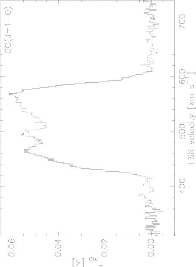
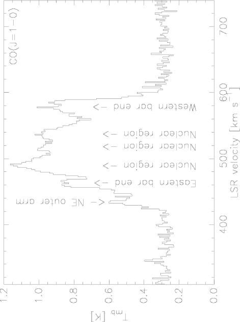
Figure 1: Left: Global CO($J$=1–0) spectrum. Right: Peak intensity CO($J$=1–0) spectrum.

By adding the CO($J$=1–0) spectra (from the raw data cube) in concentric, 20″ wide annuli (compensated for inclination and position angle and centered on the IR nucleus, see Table 1), we produced the spectra in Fig. 3. They show how the average CO($J$=1–0) velocity-integrated intensity changes with galactocentric radius (which is indicated, in arc-seconds, in the upper right corner of each panel). The coverage in the map is complete to a radius of 229″.

4.1.2 The CO($J$=2–1) spectra

The global and peak intensity CO($J$=2–1) spectra show characteristics very similar to those of the CO($J$=1–0) data, Fig. 2 [since the CO($J$=2–1) spectra were obtained with two different spacings, we regridded these data to a common 11″ spacing before producing the spectra in Fig. 2]. The main difference is that the peak intensity spectrum is brighter than the corresponding CO($J$=1–0) spectrum. This is most likely an effect of the emitting objects being smaller than the CO($J$=1–0) beam.

In Table 4 we summarize the characteristics of the global spectra. The global line intensity ratio $R_{21}\equiv\int{T_{\rm mb}(2-1)dv}/\int{T_{\rm mb}(1-0)dv}$ is 0.77$\pm$0.01, based on the errors from Table 4. Note that, including errors in the calibration and the main beam and error beam efficiencies, the result is 0.77$\pm$0.16. However, it should be noted that the relative calibration of the CO($J$=1–0) and CO($J$=2–1) data may be better than the absolute calibration and hence the error in their ratio can be smaller than indicated by the absolute error.

Table 4: Peak intensities, velocity-integrated intensities (with errors), intensity-weighted velocities, and equivalent widths of the global CO($J$=1–0) and CO($J$=2–1) spectra in Figs. 1 and 2. The errors are estimated from the noise levels. In the column for integrated intensities we also show the absolute errors.

	Peak	Integral	Centroid	Eq. width
	[K]	[K km s-1]	[km s-1]	[km s-1]
CO($J$=1–0)	0.061	8.18$\pm$0.04$\pm$0.82	515$\pm$1	134$\pm$1
CO($J$=2–1)	0.046	6.28$\pm$0.03$\pm$0.62	513$\pm$1	135$\pm$1

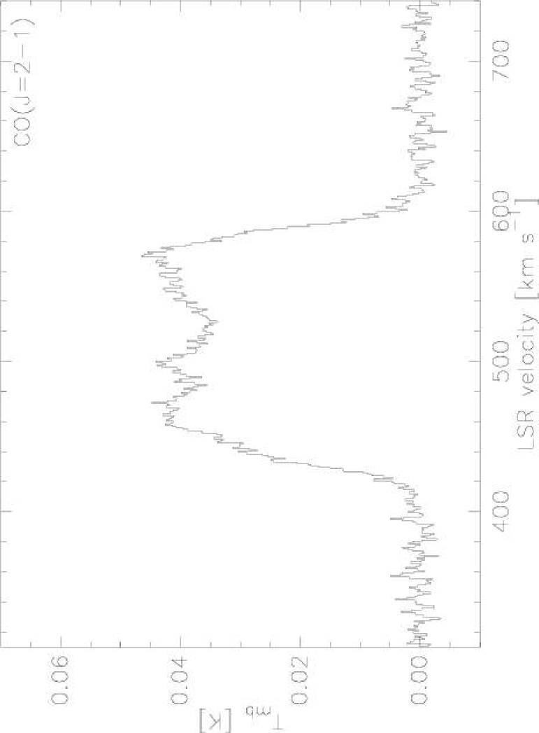
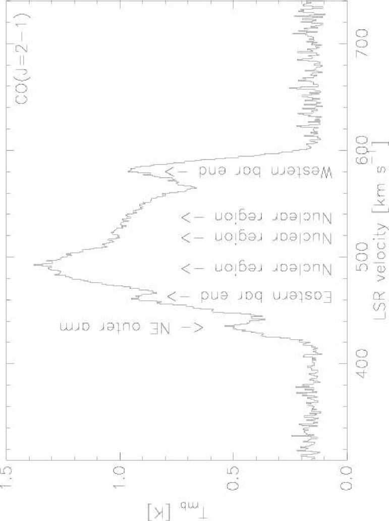
Figure 2: Left: Global CO($J$=2–1) spectrum. Right: Peak intensity CO($J$=2–1) spectrum. Before producing these spectra the CO($J$=2–1) data cube was regridded to 11″ spacing.

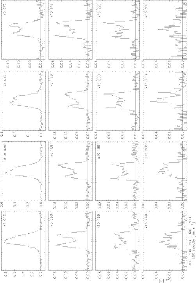
Figure 3: CO($J$=1–0) spectra produced by averaging all spectra within successive, concentric (and inclination-corrected) annuli. The average radius (in arc-seconds) of each annuli is shown in the upper right corner. The center spectrum is shown in the upper left corner, and the outermost spectrum in the lower right corner. Note that the intensity scale varies from panel to panel (the scaling factor is shown in the upper right corner of each panel). The velocity resolution has in this image been reduced to 5 km s^-1.

4.2 The maps

4.2.1 CO($J$=1–0)

Figure 4 shows maps of the CO($J$=1–0) velocity-integrated intensity (hereafter $I_{1-0}$) and the peak intensity (hereafter $T_{1-0}$) for both the convolved data set (left column) and the mem-deconvolved data set (right column). The CO($J$=1–0) emission is concentrated to the nucleus, the central part of the bar, the bar ends, and the spiral arms. The velocity-integrated intensity at the nucleus and the eastern and western bar ends are: 73, 24, and 30 K km s^-1, respectively, which is very close to the corresponding values in Crosthwaite et al. (2002): 73, 22, and 28 K km s^-1. In the mem-deconvolved data set these features are brighter due to the increased spatial resolution: at the eastern bar end we measure 49 K km s^-1, at the western bar end 52 K km s^-1, and at the nucleus the maximum $I_{1-0}$ is 235 K km s^-1 ($T_{1-0}$=2.8 K). By fitting an ellipse to the mem-deconvolved $I_{1-0}$-distribution we find that the CO peak coincides with the IR nucleus within the absolute position accuracy of our maps (3″). The axes ratio of this ellipse is 60″:29″ with a position angle of 36°. In the mem-deconvolved maps the spiral arms are resolved, and they can be followed for almost 360°. The emission in the spiral arms breaks up into regularly spaced maxima, which we interpret to be giant molecular associations (GMAs), a phenomenon previously seen in e.g. M 51 (Nakai et al., 1994). The outer arm, to the SE of the nucleus, seems somewhat disturbed in the sense that in the mem-deconvolved $T_{1-0}$ map it is possible to discern two parallel arms. Further toward the west, this arm appear to almost merge with the inner arm, which also appears to be the case on the opposite side of the galaxy (NE of the nucleus).

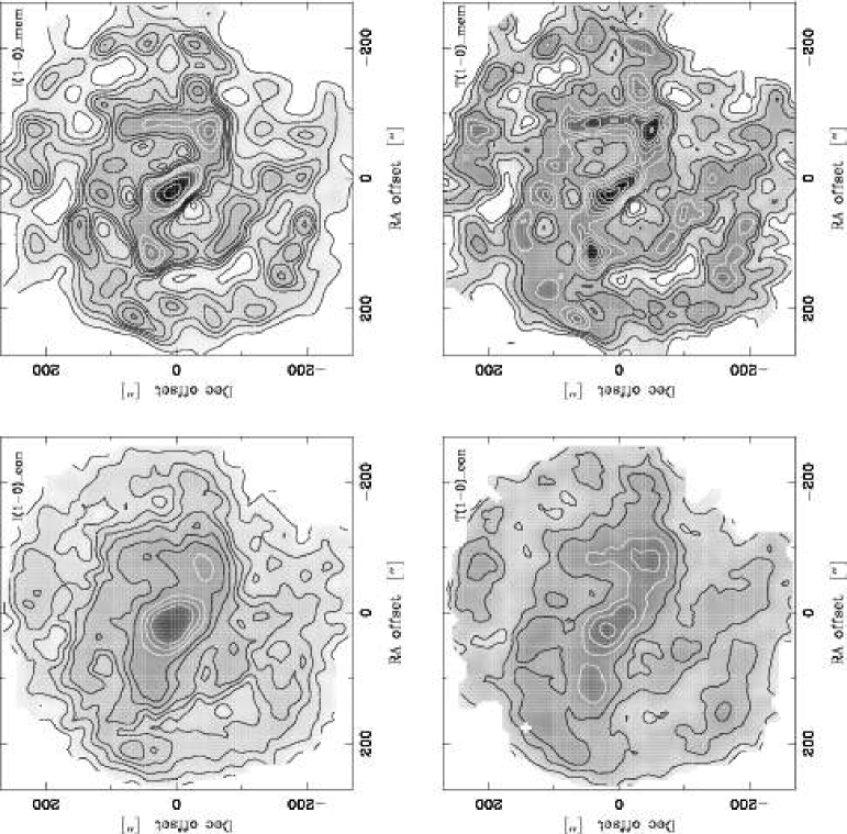
Figure 4: The CO($J$=1–0) maps. Velocity-integrated intensity in the convolved data set (resolution $\approx$49″; upper left) and in the mem-deconvolved data set (resolution $\approx$22″; upper right). Contours are: 1, 3, 5, 7, 9, 13, 18, 27 (first white contour), 37, 50, 100 and 175 K km s^-1. Maximum intensities in the convolved and mem-deconvolved maps are 127 and 235 K km s^-1, respectively. Peak intensities in the convolved data set (lower left) and in the mem-deconvolved data set (lower right). Contours are: 0.05, 0.1, 0.2, 0.3, 0.5 (first white contour), 0.7, 0.9, 1.2, 1.5, 2.0 and 2.5 K. Peak intensity at the center are 1.4 and 2.8 K for the convolved and deconvolved set, respectively.

Rand et al. (1999) (hereafter RLH) mapped the CO($J$=1–0) emission in the inner eastern arm using the OVRO Millimeter Array (spatial resolution 6$\aas@@fstack{\prime\prime}$5 $\times$ 3$\aas@@fstack{\prime\prime}$5). In Fig. 5 we show their data overlayed on our deconvolved $I_{1-0}$ map. The components close to the nucleus (components 1–5 using their nomenclature), are not prominent in our data. They are distributed along the leading edge of the bar. The reason is probably that a shock in this region creates substructures (in temperature, in density, and/or in velocity) in the CO distribution which elsewhere is smooth and therefore undetectable by an interferometer (RLH found that only 2–5% of the single-dish emission was recovered in their interferometer observations). Our eastern bar end is located between components 6 and 7, and the spiral arm segment which continues southward is located between components 9 and 10.

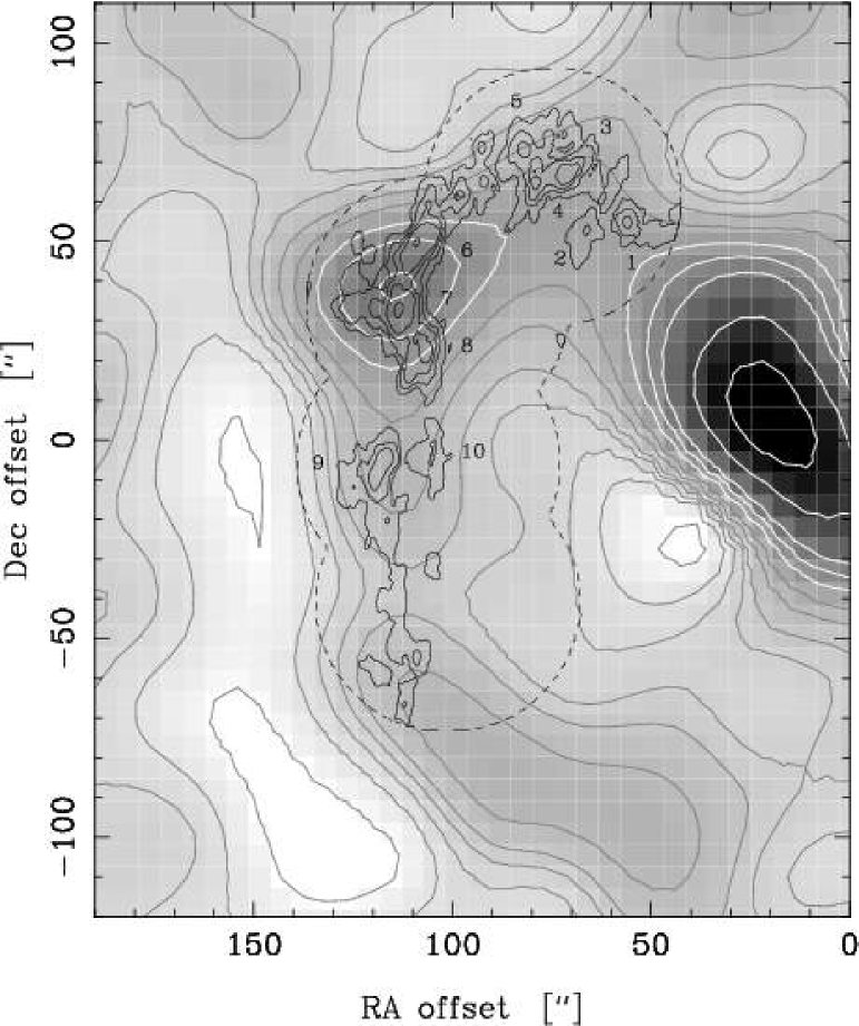
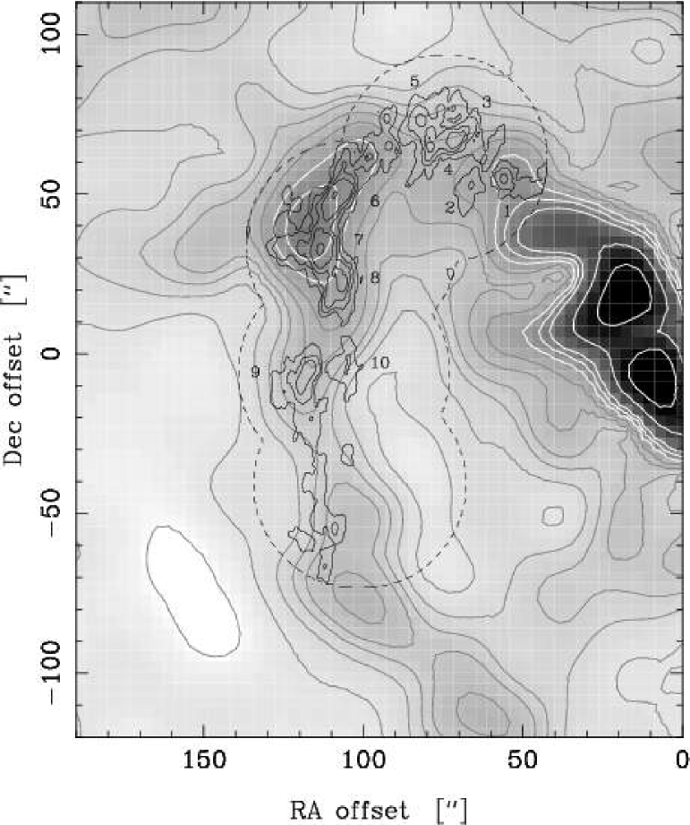
Figure 5: OVRO interferometer CO($J$=1–0) emission (thin lines) superposed on a gray+contour map of our CO($J$=1–0) [left] and CO($J$=2–1) data [right].

4.2.2 CO($J$=2–1)

The CO($J$=2–1) maps show structures very similar to those in the CO($J$=1–0) maps, however with a higher angular resolution, Fig. 6. The deconvolved $I_{2-1}$ map shows the “double nucleus” previously seen in the CO($J=3-2$) and CO($J=4-3$) lines by Petitpas & Wilson (1998). This “double nucleus” is apparent also in our raw CO($J$=2–1) data, but it is not possible to see in the convolved $I_{2-1}$ map, since this map is made using data which was both convolved (with a 15″ beam) and regridded (to 11″ spacing). Since the gray-scale and contour levels in Figs. 4 and 6 are the same, we can directly infer that the CO($J$=2–1) emission is less concentrated to the arms than the CO($J$=1–0) emission.

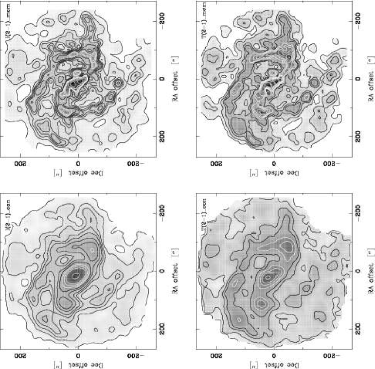
Figure 6: Same as in Fig. 4 but for CO($J$=2–1) . The contours are also the same. The resolution of the maps are 27″ and 12″ for the convolved and the mem-deconvolved data set, respectively. For the convolved data maps the values at the center are 110 K km s^-1 and 1.3 K. In the mem-deconvolved map, the nucleus breaks up into two discrete sources, with similar velocity-integrated and peak intensities: 240 K km s^-1 and 3.0 K.

5 Results and discussion

5.1 Molecular mass in M 83

The H₂ column density in external galaxies is commonly derived from the velocity-integrated CO($J$=1–0) intensity ($I_{\rm CO}=\int T_{\rm mb}dv$) using the expression

$$N({\rm H}_{2})=X_{\rm CO}\times I_{\rm CO}\ ,$$ (1)

where $X_{\rm CO}$ is a conversion factor. The actual value of this factor, and its applicability in different environments have been widely discussed, see e.g. Wilson (1995); Arimoto et al. (1996); Combes (2000); Young & Rownd (2001). In this paper we have adopted the value $X_{\rm CO}$= 2.3$\times 10^{20}$ (K km s^-1)^-1 cm^-2 (Strong et al., 1988), which is supported by the analysis done in RLH. In order to convert the measured intensities into mass surface density we used the expression

$$\Sigma({\rm H}_{2})=3.7\times I_{\rm CO}\times\cos\,i=3.3\times I_{\rm CO}{\rm\leavevmode\nobreak\ M_{\odot}\leavevmode\nobreak\ pc^{-2},}$$ (2)

where i is the inclination of the galaxy, and $I_{\rm CO}$ is given in K km s^-1 (This expression can be obtained by integrating Eq. 1). Using this conversion factor to convert the integrated intensity of the global CO($J$=1–0) spectrum (8.18 K km s^-1, Tab. 4) we find that the average (over the entire optical disk, and including the bar and the nucleus) surface mass density is 27.2 M_⊙ pc^-2, and that the total molecular gas mass within the surveyed area is 3.3$\times 10^{9}$ M_⊙.

5.2 The radial distribution

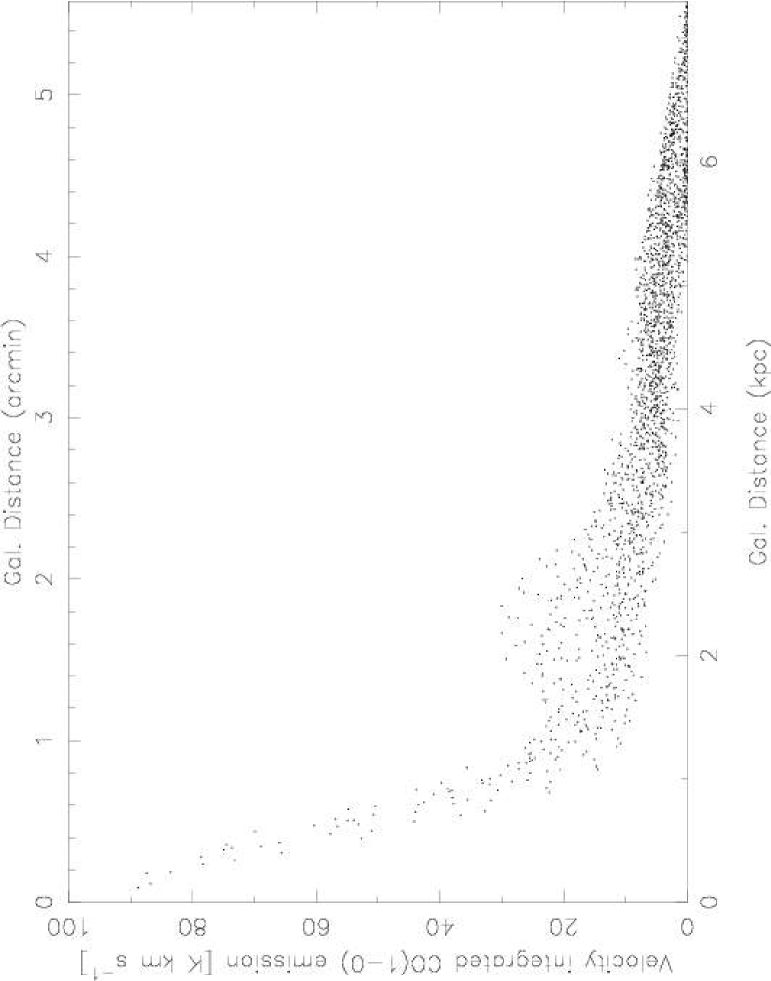
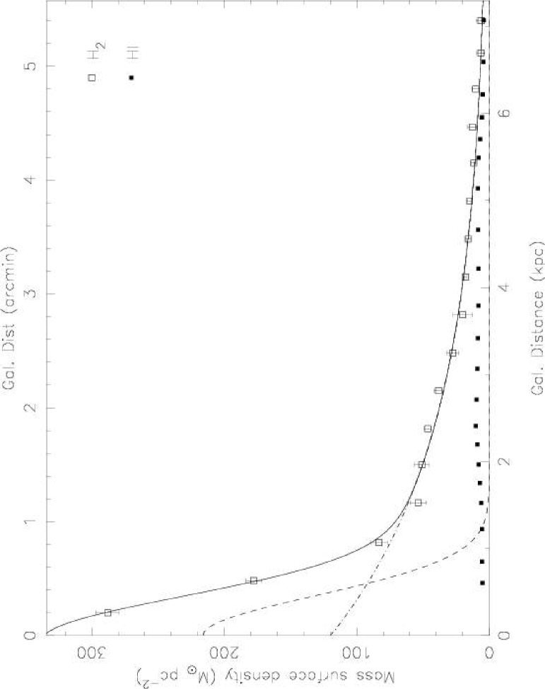
Figure 7: The CO($J$=1–0) velocity-integrated intensity versus galactocentric distance is shown in the left panel (obtained from the convolved data set). The dispersion is dominated by the arm-interarm contrast, and the bar-ends are evident at $\approx$2 kpc. In the right panel the H₂ mass surface densities are shown with formal errors (the data are taken from the spectra in Fig. 3), together with HI mass surface densities. Also shown, as a solid line, is the fit of an H₂ mass distribution described in the text. It consists of a Gaussian central part (dashed line) and an exponential disk (dash-dotted line).

5.2.1 Molecular gas

We have, using the sliding-window technique described above, calculated the velocity-integrated intensity, centroid velocity, peak intensity, and center and width of a Gaussian emission profile fitted to the spectrum for all spectra in all data cubes. The left panel of Fig. 7 shows the CO($J$=1–0) velocity-integrated intensities (obtained from the convolved data set) as a function of the (inclination-corrected) distance from the galaxy center. The scatter is dominated by the arm-interarm contrast. The data in the right panel of Fig. 7 were obtained from the integrated intensities of spectra averaged within concentric annuli (see Fig. 3 and Table 5) by converting the CO($J$=1–0) integrated intensity into mass surface density as described above. In this procedure we used the raw data set, since we needed neither the higher spatial resolution of the mem-deconvolved spectra nor the lower noise of the convolved spectra. The error bars reflect the uncertainty in the azimuthally-averaged radial distribution. To these data we fitted an H₂ mass surface density distribution which is a combination of a Gaussian component and an exponential function (for the disk),

$$\Sigma({\rm H}_{2}) = 216\exp\left[-\left(\frac{r}{649{\rm\leavevmode\nobreak\ pc}}\right)^{2}\right]+$$ (3)

$$120\exp\left[-\frac{r}{2265{\rm\leavevmode\nobreak\ pc}}\right]{\rm\ M_{\odot}\ pc^{-2}}$$

The Gaussian shape of the inner part of the distribution depends mainly on the convolution of the true distribution with the beam (the scale length 649 pc in Eq. 3 corresponds to a FWHM of 50″). The right panel of Fig. 7 shows also the mass surface density of the HI gas. These data were obtained from Tilanus & Allen (1993) (hereafter TA). The column densities in TA were obtained with the VLA, and the authors noted that their estimated total HI mass within the Holmberg radius ($0.87\times 10^{9}\leavevmode\nobreak\ {\rm M}_{\odot}$) was lower than the corresponding masses estimated by other authors using single dish observations, e.g., both Rogstad et al. (1974) and Huchtmeier & Bohnenstengel (1981) obtained about $1.6\times 10^{9}\leavevmode\nobreak\ {\rm M}_{\odot}$ (all masses recalculated to the distance 4.5 Mpc). The most probable explanation for the deficiency was, according to TA, the absence of short-spacing information. In order to compensate for this we have added the “missing” mass surface density (2.4 M_⊙ pc^-2) to the HI data of TA. The resulting HI mass surface densities are still low and typically H₂ gas constitute about 70% of the total mass of neutral hydrogen (H₂ + HI) in the disk inside 6.8 kpc.

Table 5: CO($J$=1–0) and CO($J$=2–1) velocity-integrated intensities of spectra averaged within inclination-corrected annuli. The annuli are fully sampled out to 230″. The CO($J$=2–1) data were regridded to the same spacing as the CO($J$=1–0) so that the disk was sampled in the same way for both transitions. The difference in angular resolution in the data sets has an effect on the response at the center. The errors (1$\sigma$) does not include the calibration uncertainty.

radius	$I_{1-0}$	error	$I_{2-1}$	error	#spectra
[″]	[K km s-1]	[K km s-1]	[K km s-1]	[K km s-1]	in annuli
12	87.7	2.1	98.1	0.8	9
29	53.0	1.2	51.6	0.5	27
49	25.4	1.8	19.1	0.7	49
70	15.5	1.6	10.2	0.7	67
90	15.6	1.6	11.0	0.4	85
109	14.2	0.8	11.5	0.7	100
129	11.7	0.9	8.2	0.4	126
149	7.9	1.1	5.7	0.8	141
169	6.3	1.2	4.3	0.6	157
189	5.4	0.2	3.6	0.8	181
209	4.8	0.5	3.6	0.5	198
229	4.4	0.5	3.1	0.6	215
249	3.5	0.4	2.4	0.7	212
268	3.7	0.8	2.1	0.6	155
288	3.0	0.7	1.5	0.6	102
307	2.1	0.9	$<$2.7		44

Based upon the H₂ mass surface density distribution (Eq. 3) we estimate a total molecular gas mass within a radius of 7.3 kpc (the extent of the map) of $3.5\times 10^{9}\leavevmode\nobreak\ {\rm M}_{\odot}$, and extrapolated to the Holmberg radius (7$\aas@@fstack{\prime}$3 or 9.6 kpc) the mass becomes $3.9\times 10^{9}\leavevmode\nobreak\ {\rm M}_{\odot}$ (which agrees well with the result of Crosthwaite et al. (2002), $3.7\times 10^{9}\leavevmode\nobreak\ {\rm M}_{\odot}$ (cf. also to the result $3.3\times 10^{9}\leavevmode\nobreak\ {\rm M}_{\odot}$ that was derived in Sect. 5.1 using the velocity-integrated intensity in the global spectrum). This is more than twice the total HI mass within the same galactocentric radius. It should, however, be noted that 80% of the HI mass in M 83 is found outside the Holmberg radius (Huchtmeier & Bohnenstengel, 1981). As a comparison, the stellar mass of M 83 is $\sim$ 37$\times 10^{9}\leavevmode\nobreak\ {\rm M}_{\odot}$, given V${}_{T}^{0}$=7.37 (de Vaucouleurs et al., 1992) and assuming a mass-to-light ratio of 2.

In the Gaussian/exponential disk decomposition the major part of the molecular gas mass within the Holmberg radius lies in the disk, $3.6\times 10^{9}\leavevmode\nobreak\ {\rm M}_{\odot}$. Lord (1987) made CO($J$=1–0) observations in 21 positions in the central parts of M 83, and he estimated the total molecular gas mass within 115″ to be 1.2$\times 10^{9}\leavevmode\nobreak\ {\rm M}_{\odot}$ (we have compensated for the difference in $X_{\rm CO}$ and distance). Our H₂ distribution gives 1.4$\times 10^{9}\leavevmode\nobreak\ {\rm M}_{\odot}$.

5.2.2 Comparison with data at other wavelengths

In Fig. 8 we compare the CO radial distributions with corresponding photometry data in the B, K, and H$\alpha$ bands. The B and H$\alpha$ data come from Talbot et al. (1979), and the K data from Adamson et al. (1987). The scale lengths of the various tracers compare well over most of the radial range, but the comparatively low spatial resolution affects the CO curves in the central region and at the bar ends. The latter are responsible for the peaks at $\sim$120″. We have fitted a single exponential to the data in the radial range 140″–240″, which corresponds to the region outside the bar but inside the area where our CO survey is complete. The scale lengths are: 135$\pm$14″, 126$\pm$16″, 112$\pm$20″, 100$\pm$14″ and 132$\pm$35″ for CO($J$=1–0), CO($J$=2–1), K, B, and H$\alpha$, respectively (the errors of the latter three do not include the measurement errors). Thus, the disk scale lengths are, within the errors, the same for these star formation tracers.

The CO intensities decrease exponentially over the entire surveyed area, and we do not observe the sharp cut-off at 4$\aas@@fstack{\prime}$5 seen by Crosthwaite et al. (2002). In fact, we find CO emission with $I_{1-0}$ $\approx$ 1 K km s^-1 in selected spectra as far from the nucleus as 5$\aas@@fstack{\prime}$5.

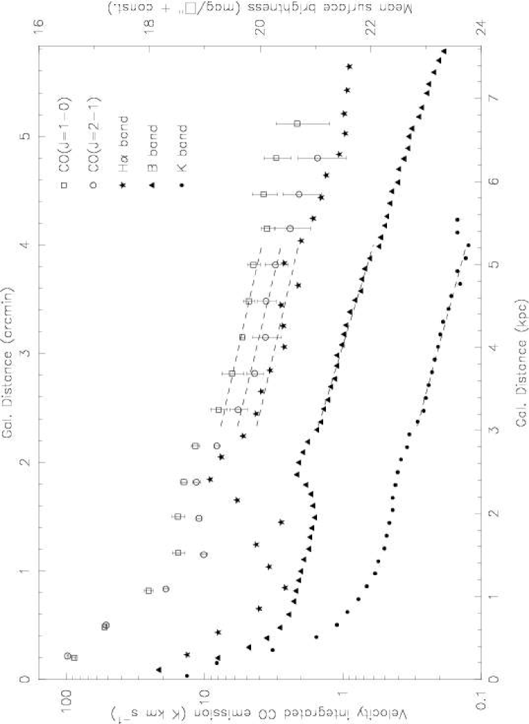
Figure 8: Azimuthally-averaged CO($J$=1–0) and CO($J$=2–1) velocity-integrated intensity (cf. Table 5) in annular zones compared to surface brightnesses in the H$\alpha$, B, and K filters. Note how the bar ends appear as a bump at 120″ in the distributions. The spatial resolution of the CO($J$=2–1) is better than that of the CO($J$=1–0) data, which results in the difference in slopes of the inner parts of these distributions. The dashed lines show the fits of exponentials discussed in the text.

5.3 Brightness distributions

We find that in the mem-deconvolved map the average CO($J$=1–0) intensity in the arms is about 2.5 times higher than in the interarm regions. Assuming a direct proportionality between CO emission and mass surface density, this agrees well with the lower limit of the arm–interarm mass surface density ratio, 2.3, found by RLH using purely kinematical arguments.

In Fig. 9 we show the mem-deconvolved CO($J$=1–0) velocity-integrated intensity map superposed on a true-color image. This image is a composite of three images in the filters B, V, and R, rendered as blue, green, and red, respectively. These images have been obtained at the ESO Danish 1.54 m telescope by Sören Larsen and the data are described in Larsen & Richtler (1999). On the large scale the CO($J$=1–0) emission follows the dust lanes, both in and between spiral arms, but at some locations the CO($J$=1–0) emission is displaced toward the regions where star formation takes place (Wiklind et al., 1990). Most notably, in the inner spiral arm on the eastern side, the CO($J$=1–0) ridge is located downstream of the dust lane with a separation of about 10–15″ (also shown in RLH), as are the HI and H$\beta$ emissions as shown by TA. We note that in general the OB associations straddle the rims of the CO($J$=1–0) emission concentrations, presumably due to extinction in combination with the photodissociation by the young stellar population. The outer and inner spiral arms appear to connect at several locations, and these connection regions often show an increased number of OB associations. The “Gould belt structure”, at (1$\aas@@fstack{\prime}$75,–2$\aas@@fstack{\prime}$25) in the coordinate system of Fig. 9, is such a region (Comerón, 2001).

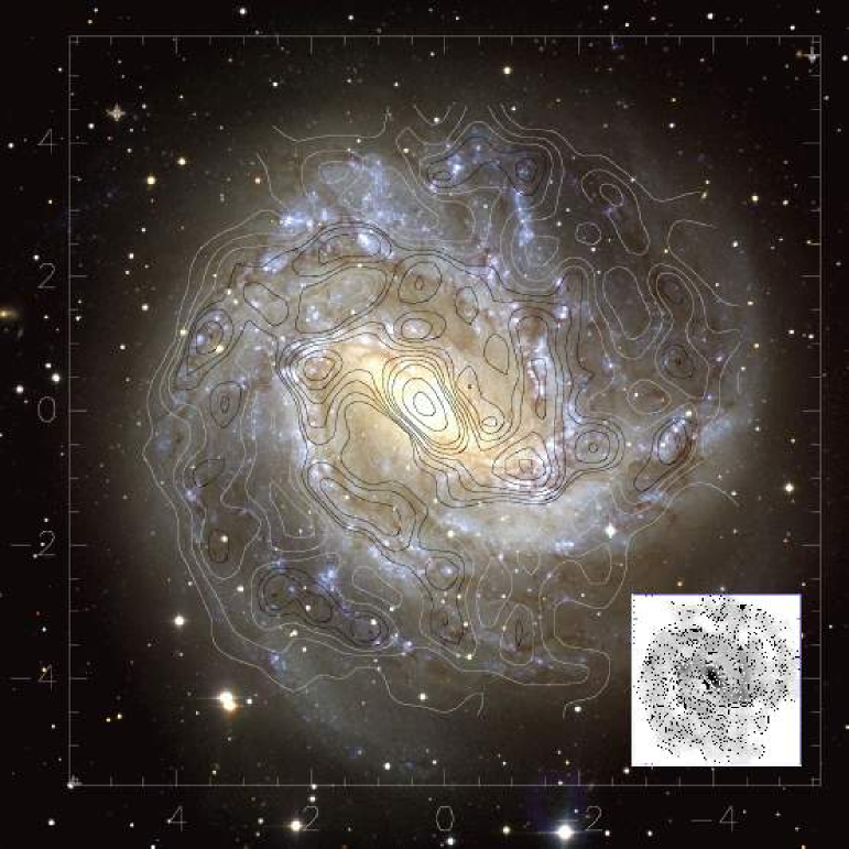
Figure 9: The mem-deconvolved velocity-integrated CO($J$=1–0) intensity as contours superposed on an RGB-map produced from images in B, V, and R. The optical images were obtained by Sören Larsen at the ESO Danish 1.5 m telescope on La Silla, Chile. Three stars have been used for image alignment. These are located in the lower left corner and in both upper corners and are marked with crosses. The inset shows the CO($J$=1–0) map in gray-scale.

Figure 10 shows the CO($J$=2–1) velocity-integrated intensity as contours on an RGB image, where the colors represent star formation (H$\alpha$; red), infrared emission (I band; green), and dust lanes (filters V–I; blue). In the disk, the observed CO($J$=2–1) brightness distribution strengthens the conclusions drawn from the CO($J$=1–0) emission. In the central region the higher angular resolution at the CO($J$=2–1) frequency reveals additional details. There are two central nuclear components relatively symmetrically placed on opposite sides of the IR center. At these locations the dust lanes, on the leading edges of the bar, attach to the nuclear ring seen in J–K by Elmegreen et al. (1998). Their color difference map (V–I) shows an area of high dust extinction at the location of the NE component, whereas at the SW component there appears to be relatively small amounts of dust. It appears as if the NE CO component lies above the disk (or the bulge) and the SW CO component lies below or behind the same. This was also concluded by Sofue & Wakamatsu (1994) based on similar data. Along the bar, the CO($J$=2–1) emission follows the dust lanes on the leading edges. In the disk the CO emission traces the H$\alpha$ emission very well, although there are regions with a clear anti-correlation, i.e., substantial CO emission but none, or very weak, H$\alpha$ emission, such as the peak at about half an arcminute west of the nucleus.

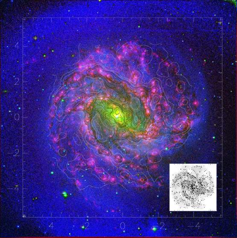
Figure 10: The mem-deconvolved CO($J$=2–1) velocity-integrated intensity as contours on an RGB image where the colors red, green and blue represent star formation (H$\alpha$), infrared emission (I band), and dust lanes (filters V–I), respectively. The inset shows the CO($J$=2–1) map in gray-scale.

Figure 11 shows the CO($J$=1–0) velocity-integrated intensity on a gray-scale image of the HI column density (data kindly provided by R.P.J. Tilanus and R.J. Allen). The angular resolution of the HI map is slightly better than that of the CO map. The CO emission (which is assumed to be linearly proportional to the H₂ mass surface density intensity) and the HI column density follow each other closely, with one outstanding exception: the nucleus, where very little HI is present. At some places in the disk the H₂ and HI maxima are displaced from each other, but there is no apparent systematic trend that H₂ is outside HI or vice verse. In general, the separations are of the order of 3-9$\arcsec$, which is small compared to the resolution in these maps (23$\arcsec$).

Local minima in the HI and H₂ gas surface densities also correlate well. At (50$\arcsec$,180$\arcsec$) in the coordinate system of Fig. 11, marked minima can be seen in both H₂ and HI. The total gas surface density in this area is about 3–6 M_⊙ pc^-2, of which only $\approx$1 M_⊙ pc^-2 is in the form of molecular gas. Such low mass surface densities should not give rise to any massive star formation, and indeed, the H$\alpha$ image shows very little emission here.

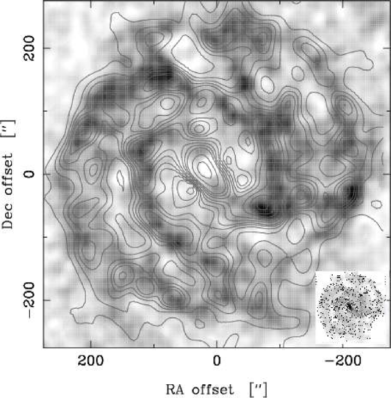
Figure 11: The mem-deconvolved velocity-integrated CO($J$=1–0) intensity as contours on an HI column density map (gray-scale) of roughly similar resolution ($\approx$20″). The HI data comes from TA. The inset shows the CO($J$=1–0) map in gray-scale.

Figure 12 compares the H₂ (as probed by the CO($J$=2–1) emission) and the HI gas in more detail, the resolution being $\approx$ 10$\arcsec$. In the main disk the CO($J$=2–1) emission and HI emission follow each other closely and several of the concentrations in the CO($J$=2–1) emission are also seen in the HI distribution. Again the exception is the nuclear region. The mass surface density of HI at the two nuclear components differ markedly: the SW component has a peak mass surface density of 6 M_⊙ pc^-2, while at the center of the NE component HI is actually seen in absorption against a nuclear continuum source, which again speaks in favor of the idea that the SW and NE components lie on different sides of the disk (or a bulge). The mass surface density of HI at the center is very much lower than that of H₂, where the highest value in the $I_{1-0}$ map corresponds to $\approx$750 M_⊙ pc^-2. In the $I_{1-0}$ map it is not possible to distinguish the separate nuclei due to the relatively low spatial resolution and the coarse grid. However, using the average 2–1/1–0 line ratio (see Sect. 5.4), the mass surface density is $\sim$1100 M_⊙ pc^-2 for each of these components. As the physical properties of the molecular gas in the center may differ from that in the disk, application of the standard conversion factor may lead to an erroneous result. Indeed, it is likely that at least part of the emission in the center comes from a diffuse and non-virialized component. This would lead to an overestimate of the molecular gas mass (Papadopoulos & Allen, 2000).

The explanation for the nice correlation may be that the HI is mostly a dissociation product, as TA discuss. A smooth distribution of ‘primordial’ HI gas would not be detected in the interferometer observations (in which roughly 50% of the HI gas was detected) while HI produced as an effect of dissociation of molecular gas in the neighborhood of star formation would be localized, and therefore detected by the interferometer.

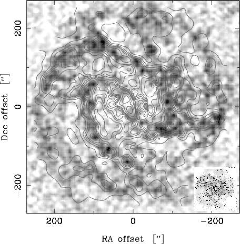
Figure 12: The mem-deconvolved velocity-integrated CO($J$=2–1) intensity as contours on an HI column density map (gray-scale) of roughly similar resolution ($\approx$12″). The HI data comes from TA. The inset shows the CO($J$=2–1) map in gray-scale.

5.4 The CO ($J$=2–1)/($J$=1–0) line intensity ratio

We have created a map of the CO($J$=2–1)/($J$=1–0) line intensity ratio, $R_{21}$, at 49″ resolution. The mean value over this map is 0.72$\pm$0.19, which is within the errors the value derived from the velocity-integrated intensities in Table 4. Crosthwaite et al. (2002) estimate a ratio of 1.1$\pm$0.2, which we suspect is higher than ours because they have not corrected their CO($J$=2–1) data for the error beam contribution (considering the main beam efficiency of the NRAO 12 m telescope at this frequency, $\approx$0.56, the error beam is likely to be comparable to that of the SEST). In the nuclear region and along the bar the ratio is 0.83$\pm$0.04. The $R_{21}$ map shows also that on the arms, the line intensity ratio is lower than in the interarm regions. This is illustrated in Figure 13, where $R_{21}$ is plotted as a function of radius in a $45\degr$ wide sector of the galaxy (position angle 90°–135°). In order to quantify and compare the ratio on the arms to that in the interarm regions, we have selected two sectors where the arms are well separated. The position angle of these sectors are: 90°–135° (SE) and 270°–315° (NW). In these sectors we selected spectra belonging to the inner, outer and inter-arm regions, and averaged them separately. Finally, “arm”-spectra were created by taking the average of the inner and outer arm spectra in the two respective sectors. From these eight spectra, four ratios were calculated. Assuming our error beam is correct (Sect. A), the line ratio is significantly lower on the arms: 0.59$\pm$0.04 (SE) and 0.69$\pm$0.04 (NW) compared to the ratio in the interarm region 0.88$\pm$0.17 (SE) and 0.98$\pm$0.21 (NW) (the errors are 3$\sigma$ and are estimated from the noise level in the spectra). We believe that this is an effect of a (partly) different cloud component in the interarm regions, where the heating of the gas is more efficient than in the dense arm cloud complexes. As a note: We have also calculated the $R_{21}$ value for the mem-deconvolved CO($J$=1–0) and CO($J$=2–1) maps at the common resolution 30″. The arm value is roughly the same (0.6$\pm$0.1), but the interarm value is higher, 1.3$\pm$0.3.

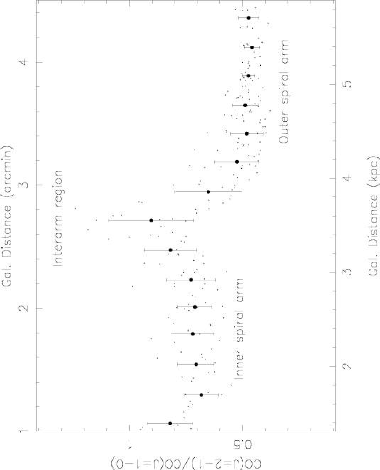
Figure 13: The CO ($J$=2–1)/($J$=1–0) line intensity ratio, $R_{21}$, as a function of galactocentric radius. The interarm region shows a clear trend of increased line ratio. The data are taken from a $45\degr$ wide sector SE of the nucleus (position angle 90°–135°).

By averaging $R_{21}$ in concentric annuli, we find a trend in the line intensity ratio in the sense that it decreases with galactocentric distance, Fig. 14 (this is also indicated in Fig. 8). In particular, the lower envelope of the $R_{21}$-values is clearly decreasing. A similar difference between the $R_{21}$ line ratio in the disk and towards the nucleus has previously been shown to exist in our Galaxy (Sawada et al., 2001). The wiggles in Fig. 14 can be associated with features in the $R_{21}$ map. The nucleus appears to be surrounded by a ring of excited gas, which is reflected as a bump in the radial distribution. The bar ends and inner arms are reflected as a flat region at $\approx$120–150$\arcsec$ , while the low $R_{21}$-values in the outer arms suppresses the average $R_{21}$-ratio in the range 200–300″.

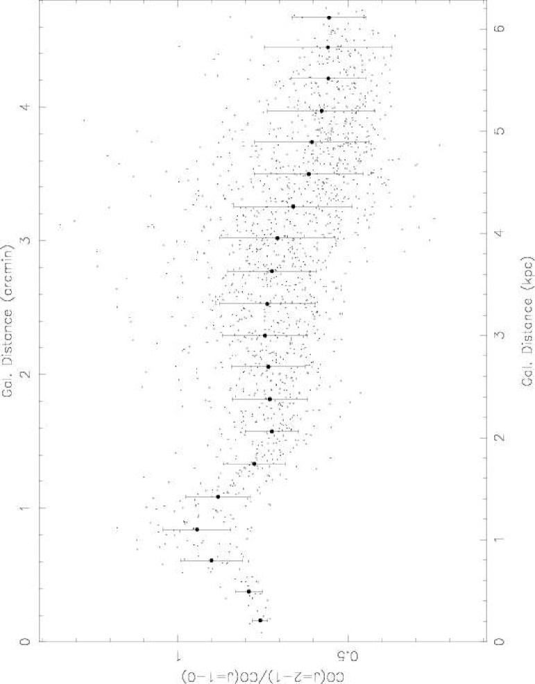
Figure 14: The CO ($J$=2–1)/($J$=1–0) line intensity ratio for individual positions (dots) and the azimuthally averaged ratio (with error bars) in annular zones in the plane of the galaxy.

6 Conclusions

We have mapped, in over-sampling mode, the CO($J$=1–0) and CO($J$=2–1) brightness distributions over the entire optical disk of M83. Significant corrections for an error beam have been applied to the CO($J$=2–1) data. A mem-method has been used to increase the angular resolution of the data.

We find that:

i) the CO emission is strongly peaked toward the nucleus, which splits up into two components in the CO($J$=2–1) data. Also the bar ends are prominent. The CO emission follows the leading edges of the bar.

ii) Molecular gas spiral arms are clearly identified, and they trace, in most cases, the dust lanes. There are frequent “bridges” between spiral arms, and in some areas the arms are clearly disturbed.

iii) An average arm–interarm brightness contrast of about 2.5 is found for the CO($J$=1–0) line.

iv) The CO ($J$=2–1)/($J$=1–0) line ratio, which is about 0.77 on average, differ between the arm and interarm regions. It is significantly higher in the latter.

v) Regularly spaced molecular gas concentrations of mass $\approx$10⁷ M_⊙ lie along the arms.

vi) The estimated total molecular gas mass is 3.9$\times$10⁹ M_⊙, and within 7.3 kpc the H₂ mass dominates over that of HI by a factor of more than two. The estimated gas/stellar mass ratio is $\approx$0.1 in the optical disk.

vii) The CO and HI emissions are very well correlated in the optical disk, and frequently concentrations of the two gas components coincide.

viii) The CO radial brightness distribution in the disk follows that of other starformation tracers as H$\alpha$ emission, and continuum light in the B and K filters. The estimated scale length, of a fitted exponential, is about 120$\arcsec$, corresponding to 2.6 kpc at the adopted distance.

Appendix A Error beam

The beam pattern of a radio telescope is affected by its surface accuracy. This means that the power received in the error beam may very well be comparable to the power received in the main beam. For sources that are compact relative to the extent of the beam, it is relatively easy to compensate for this underestimate of the true flux: The measured antenna temperature ($T_{\rm A}^{*}$) is simply divided by the main beam efficiency, $\eta_{\rm mb}$, to attain the main beam brightness temperature ($T_{\rm mb}$). The main beam efficiency is usually well known and can be found in the user manual of the different telescopes. For extended sources, the situation is more complex, since the antenna may receive power not only from the main beam. If the size of the error beam is comparable to the extent of the source, a simple multiplication of $(\eta_{\rm mb})^{-1}$ will overestimate the flux at the position where the measurement is done. If the antenna pattern is well known, it is possible to calculate how the beam couples to the source and thus compensate for this effect. Unfortunately, the antenna pattern for SEST has never been measured properly, so this was not an option for us. Instead we devised a procedure to remove the impact of the error beam, using our own data set to estimate the strength and size of the error beam pattern.

Nearly all CO($J$=2–1) spectra did show two components: one narrow line, that agrees with the width and center velocity of the CO($J$=1–0) spectra at the same position and another, broader, component that is picked up by the error beam. By studying these broad wings in a number of spectra in the deconvolved CO($J$=2–1) data set and by comparing with spectra in data cubes convolved with different FWHPs, we estimated that the size of the error beam at 230 GHz is of the order of 200″. This is in good agreement with the error beam size of 3′, which was assumed by Johansson et al. (1998).

In order to try to estimate the impact of the error beam we produced a data set where we convolved the mem-deconvolved data set with a 200″ Gaussian profile. In each position an automated process, using the sliding window technique, calculated the velocity-integrated intensity in the region of the extended wings [i.e. outside the velocity range where we have seen emission in the CO($J$=1–0) data] in both the deconvolved cube and in the 200″ convolved cube. The ratio between these intensities corresponds to the fraction of the available emission which is picked up by the error beam. We will refer to this as the error beam efficiency. In principle, the error beam efficiency must lie in the interval 0.1–0.5, since the main beam efficiency is 0.5 and the moon beam efficiency is 0.9. Some values of our error beam efficiency estimates are higher than 0.5. This happens in regions where the emission in the main beam falls outside the expected velocity range (e.g., in regions with exceptionally strong streaming motions or wide emission profiles), leading to an over-estimation of the flux in the wings. An attempt to make the window wider had a negative impact on the results since we were left with fewer channels to calculate the velocity-integrated emission in the wings. Neglecting values above 0.5, we found that the error beam efficiency was on average 0.27$\pm$0.11.

Figure 15 shows the original spectrum, the 200″ convolved spectrum (scaled with the error beam efficiency), and the resulting (cleaned) spectrum after subtraction of the two previous spectra, in four typical positions. The convolved spectra reproduces the shape of the wings very well, and the shape of the cleaned spectra resembles the corresponding CO($J$=1–0) spectra (not shown).

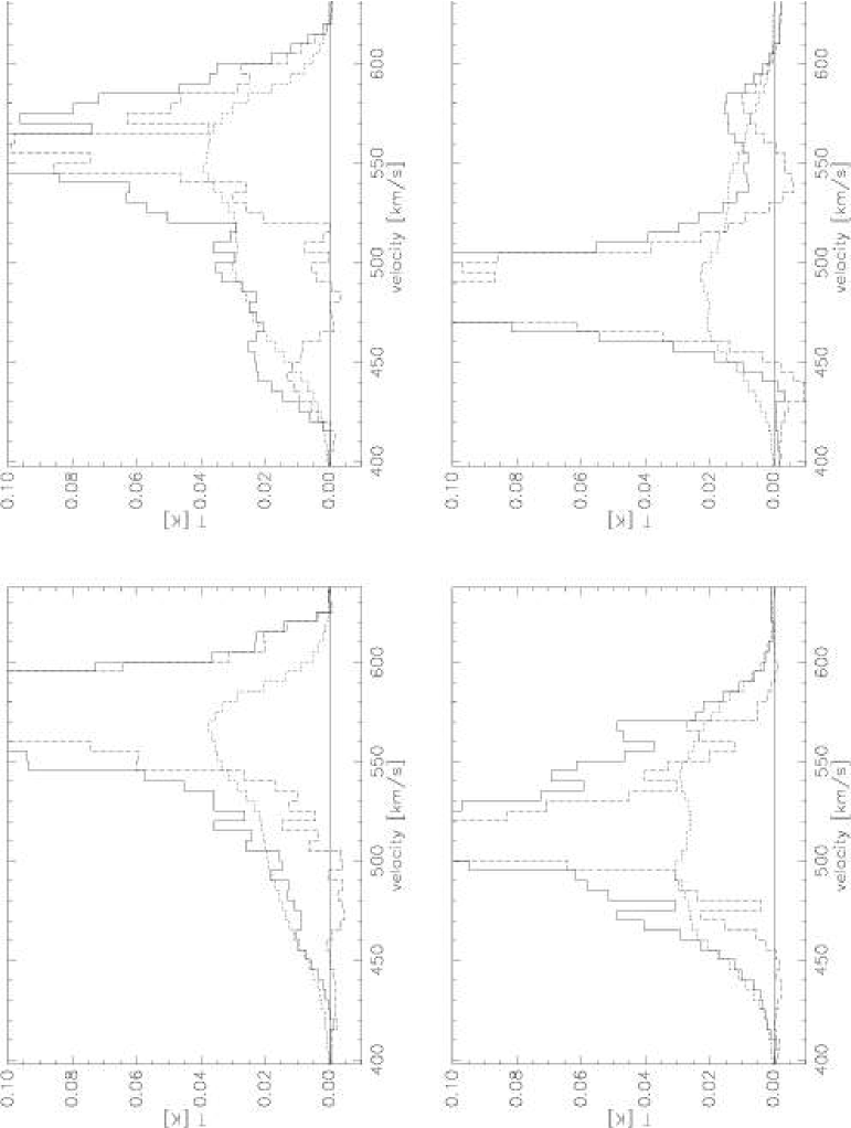
Figure 15: These spectra show the original spectra (solid lines), 200″ convolved spectra (short-dashed lines) and subtracted spectra (long-dashed lines) in four typical positions. The coordinates with respect to the map center is, from upper left to lower right, (-42,-70), (-42,0), (-42,70) and (-42,140). The 200″ convolved spectra are scaled with the derived error beam efficiency.

We have corrected the convolved and the mem-deconvolved data sets for this error by subtracting the error beam contribution for each individual spectrum. Based on the previous result, we took a conservative approach and fixed the error beam contribution to 0.27. In principle, we could have let this ratio vary from spectrum to spectrum by fitting the 200″-convolved spectrum to the extended wings, but this would have introduced other, not easily controlled, errors.

References

- Aalto et al. (1999) Aalto, S., Hüttemeister, S., Scoville, N. Z., & Thaddeus, P. 1999, ApJ, 522, 165
- Adamson et al. (1987) Adamson, A. J., Adams, D. J., & Warwick, R. S. 1987, MNRAS, 224, 367
- Arimoto et al. (1996) Arimoto, N., Sofue, Y., & Tsujimoto, T. 1996, PASJ, 48, 275
- Booth et al. (1989) Booth, R. S., Delgado, G., Hagstrom, M., et al. 1989, A&A, 216, 315
- Calzetti et al. (1999) Calzetti, D., Conselice, C. J., Gallagher, J. S., & Kinney, A. L. 1999, AJ, 118, 797
- Casoli et al. (1998) Casoli, F., Sauty, S., Gerin, M., et al. 1998, A&A, 331, 451
- Combes (1991) Combes, F. 1991, ARA&A, 29, 195
- Combes (2000) Combes, F. 2000, in Euroconference ”The Evolution of Galaxies” I- Observational Clues, ed. J. Vilchez, G. Stasinska, & E. Perez, 7318
- Combes et al. (1978) Combes, F., Encrenaz, P. J., Lucas, R., & Weliachew, L. 1978, A&A, 67, L13
- Comerón (2001) Comerón, F. 2001, A&A, 365, 417
- Comte (1981) Comte, G. 1981, A&AS, 44, 441