Non-linear evolution of the cosmological background density field as diagnostic of the cosmological reionization

Abstract

We present constraints on the cosmological and reionization parameters based on the cumulative mass function of the Ly-$\alpha$ systems. We evaluate the formation rate of bound objects and their cumulative mass function for a class of flat cosmological models with cold dark matter plus cosmological constant or dark energy with constant equation of state encompassing different reionization scenarios and compare it with the cumulative mass function obtained from the Ly-$\alpha$ transmitted flux power spectrum.
We find that the analysis of the cumulative mass function of the Ly-$\alpha$ systems indicates a reionization redshift $z_{r}=24.2\pm 4$ (68%CL) in agreement with the value found on the basis of the WMAP anisotropy measurements, setting constraints on the amplitude of the density contrast, $\sigma_{8}=0.91\pm 0.04$ (68%CL), similar to those derived from the X-ray cluster temperature function.

Our joint analysis of Ly-$\alpha$ cumulative mass function and WMAP anisotropy measurements shows that the possible current identification of a running of the slope, $dn_{s}/d{\rm ln}k\neq 0$, at $k_{p}$=0.05Mpc^-1 (multipole ${\it l}\approx 700$) is mainly an effect of the existing degeneracy in the amplitude-slope plane at this scale, the result being consistent with the absence of running, the other constraints based on WMAP data remaining substantially unchanged.

Finally, we evaluate the progress on the determination the considered parameters achievable by using the final temperature anisotropy data from WMAP and from the forthcoming Planck satellite that will significantly improve the sensitivity and reliability of these results.

This work has been done in the framework of the Planck LFI activities.

1 Introduction

The cosmological density background is assumed to have been seeded at some early epoch in the evolution of the Universe, inflation being the most popular of the current theories for the origin of the cosmological structures (see e.g. Kolb & Turner 1990, Linde 1990).
Measurements of the Cosmic Microwave Background (CMB) anisotropies present at the epoch of the recombination at large scales ($R\,\lower 2.0pt\hbox{${>\atop\hbox{\raise 4.0pt\hbox{$\sim$}}}$}\,8h^{-1}$Mpc), always outside the horizon during the radiation-dominated era, carry precious information on the power spectrum of density field. Moving to intermediate and small scales the background density field encodes information related to the non-linear evolution of the gravitational clustering, the time evolution of the galaxy bias relative to the underlying mass distribution (see e.g. Hoekstra et al. 2002, Verde et al. 2002), and the magnitude of the peculiar motions and bulk flows in the redshift space (Kaiser 1987). At these scales the spectrum of the background density field can be constrained by complementing CMB measurements with other astronomical data (see Kashlinsky (1998) for the evaluation of the spectrum of the density field from a variety of astronomical data on scales 1$h^{-1}$Mpc $\leq$ R $\leq$ 100$h^{-1}$Mpc ).

In particular, on scales less then 5 $h^{-1}$Mpc the spectrum of the density field can be constrained by using observations of the spatial distribution of high-redshift collapsed objects as quasars and galaxies and information on their macroscopic properties (Efstathiou & Ress 1988, Kashlinsky & Jones 1991, Kashlinsky 1993). The detection of high-z quasars by the Sloan Digital Sky Survey (Becker et al. 2001, White et al. 2003, Fan et al. 2003) and by the Keck telescope (Vogt et al. 1994, Songaila & Cowie 2002) as well as the detection of high-redshift galaxies (see Kashlinsky (1998) and the references therein) are indications about the existence of such early collapsed objects at redshifts between 2 and 6, on mass scales of $\sim$ 10¹⁰M_⊙.
The rms mass fluctuations over a sphere of radius of 8$h^{-1}$Mpc, $\sigma_{8}$, fixes the amplitude of the density field power spectrum and then determines the redshift of collapse, $z_{c}$, of an object with a given mass-scale. Consequently, the observation of such objects can set significant constraints on different cosmological theories.
Recently, the WMAP  team (Spergel et al. 2003, Verde et al. 2003) highlighted the relevance of complementing the CMB and LSS measurements with the Ly-$\alpha$ forest data (the absorptions observed in quasar spectra by the neutral hydrogen in the intergalactic medium) in constraining the cosmological parameters (Croft et al. 1998; Zaldarriaga et al. 2003 and references therein) and the shape and amplitude of the primordial density field at small scales.

In this paper we investigate the dynamical effects of the non-linear evolution of the density field implied by the high-z collapsed objects as diagnostic of the reionization history of the Universe. The reionization is assumed to be caused by the ionizing photons produced in star-forming galaxies and quasars when the cosmological gas falls into the potential wells caused by the cold dark matter halos. In this picture the reionization history of the Universe is a complex process that depends on the evolution of the background density field and of the gas properties in the intergalactic medium (IGM) and on their feedback relation. The evolution of the background density field, that determines the formation rate of the bound objects, is a function of the grow rate of the density perturbations and depends on the assumed underlying cosmological model. The evolution of the gas in the IGM is a complex function of the gas density distribution and of the gas density-temperature relation. The latter is related to the spectrum (amplitude and shape) of the ionizing radiation, to the reionization history parametrized by some reionization parameters (the reionization redshift, $z_{r}$, and the reionization temperature, $T_{r}$), and to the assumed cosmological parameters.
As shown by hydrodynamical simulations (Cen et al. 1994; Zhang et al. 1995; Hernquist et al. 1996; Theuns et al. 1998), the gas in the IGM is highly inhomogeneous, leading to the non-linear collapse of the structures. In this process the gas is heated to its virial temperature. The photoionization heating and the expansion cooling cause the gas density and temperature to be tightly related. Finally, the temperature-mass relation for the gas in the IGM at the time of virilization determines the connection between the gas density and the matter density at the corresponding scales.

Taking advantage of the results of a number of hydrodynamical simulations (Cen et al. 1994; Miralda-Escudé et al. 2000; Chiu, Fan & Ostriker 2003) and semi-analytical models (Gnedin & Hui 1998; Miralda-Escudé, Haehnelt & Rees 2000, Chiu & Ostriker 2000), we re-assess in this paper the possibility to use the mass function of Ly-$\alpha$ systems to place constraints on spatially flat cosmological models with cold dark matter plus cosmological constant or dark energy, encompassing different reionization scenarios. We use the Press-Schechter theory (Press & Schechter 1974) to compute the comoving number density of Ly-$\alpha$ systems per unit redshift interval from the Ly-$\alpha$ transmitted flux power spectrum (Croft et al. 2002) and examine the constraints on the cosmological parameters. In our analysis we take into account the connection between the non-linear dynamics of the gravitational collapse and the properties of the gas in the IGM through the virial temperature-mass relation. We address the question of the consistency of the WMAP and Ly-$\alpha$ constraints on the cosmological parameters, paying a particular attention to the degeneracy between the running of the effective spectral index and the power spectrum amplitude. Finally, we discuss the improvements achievable with the final WMAP temperature anisotropy data and, in particular, the impact of the next CMB temperature anisotropy measurements on-board the ESA Planck  satellite.

2 Early object formation mass function

2.1 Formation rates

The most accurate way used to assess the formation rates of the high-z collapsed objects is based on numerical simulations. A valid alternative is offered by the Press-Schechter theory (Press & Schechter 1974, Bond et al. 1991) extensively tested by numerical simulations for both open and flat cosmologies (Lacey & Cole 1994, Eke, Cole & Frenk 1996, Viana & Liddle 1996).

According to the Press-Schechter theory, the fraction of the mass residing in gravitationally bounded objects is given by:

$$f_{{\rm coll}}(z)\approx\sqrt{\frac{2}{\pi}}\frac{1}{\sigma(R_{f},z)}\int_{\delta_{c}(z)}^{\infty}\exp{\left[-\frac{\delta_{c}^{2}(z)}{2\sigma(R_{f},z)}\right]}d\,\delta_{c}(z)\,.$$ (1)

Here $\delta_{c}(z)$ is the redshift dependent density threshold required for the collapse; $R_{f}$ is the filtering scale associated with the mass scale $M=4\pi R_{f}^{3}\rho_{b}/3$, $\rho_{b}$ being the comoving background density; $\sigma(R_{f},z)$ is the rms mass fluctuation within the radius $R_{f}$:

$$\sigma^{2}(R_{f},z)=\int_{0}^{\infty}\frac{d\,k}{k}\Delta^{2}(k,z)W^{2}(kR_{f})\,,$$ (2)

where W(x) is the window function chosen to filter the density field. For a top-hat filtering $W(x)=3({\rm sin}x-x{\rm cos}x)/x^{3}$ while for a Gaussian filtering $W(x)=\exp(-x^{2})$. As we do not find significant differences between the results derived by adopting the two considered window functions for some representative cases, we present in this work the results obtained by using the Gaussian smoothing. In the above equation $\Delta^{2}(k,z)$ is referred as the power variance and is related to the matter power spectrum $P(k,z)$ through:

$$\Delta^{2}(k,z)=\frac{1}{2\pi^{2}}k^{3}P(k,z)\,.$$ (3)

Motivated in the framework of the spherical collapse model and calibrated by N-body numerical simulations, the linear density threshold of the collapse $\delta_{c}(z)$ was found to vary at most by $\simeq 5$ % with the background cosmology (see e.g. Lilje 1992, Lacey & Cole 1993, Eke, Cole & Frenk 1996). However, the choice of $\delta_{c}(z)$ depends on the type of collapse. For the spherical collapse the standard choice is $\delta_{c}(0)=1.7\pm 0.1$ while for pancake formation or filament formation its value is significantly smaller (Monaco 1995). For the purpose of this work we assume that the collapse have occurred spherically and use $\delta_{c}(0)=1.686$ that is the conventional choice for the case of the flat cosmological models (Eke, Cole & Frenk 1996). The time evolution of $\delta_{c}$ depends on the background cosmology:

$$\delta_{c}(z)=\delta_{c}(0)\frac{D(z)}{D(0)}\,,$$ (4)

where $D(z)$ is the linear growth function of the density perturbation, given in general form by (Heath 1977, Carroll, Press & Turner 1992, Hamilton 2001):

$$D(a)=\frac{5\Omega_{m}}{2af(a)}\int_{0}^{a}f^{3}(a)d\,a\,.$$ (5)

Here $a=(1+z)^{-1}$ is the cosmological scale factor normalized to unity at the present time ($a_{0}=1$), $\Omega_{m}$ is the matter density energy parameter at the present time and $f(a)$ specifies the time evolution of the scale factor for a given cosmological model:

$$\frac{d\,a}{d\,t}=\frac{H_{0}}{f(a)},\hskip 11.38092ptf(a)=\left[1+\Omega_{m}\left(\frac{1}{a}-1\right)+\Omega_{de}\left(\frac{1}{a^{1+3w}}-1\right)\right]^{-1/2}.$$ (6)

In the above equation $H_{0}$ is the present value of the Hubble paramenter, $\Omega_{de}$ is the present value of the energy density parameter of the dark energy, $w=p/\rho_{de}\sim-1$ defines the dark energy equation of state, and $\Omega_{m}$ is the matter energy density parameter. Equation (6) reduces to that of a $\Lambda$CDM model for $w=-1$.

The comoving number density of the gravitationally collapsed objects within the mass interval $d\,M$ about $M$ at a redshift $z$ is given by (Viana & Liddle 1996):

$$n(M,z)d\,M=-\sqrt{\frac{2}{\pi}}\frac{\rho_{b}}{M}\frac{\delta_{c}}{\sigma^{2}(R_{f},z)}\frac{d\,\sigma(R_{f},z)}{d\,M}\exp{\left[-\frac{\delta_{c}^{2}}{2\sigma^{2}(R_{f},z)}\right]}d\,M.$$ (7)

We are interested in the formation rate of the high-z collapsed objects at a given redshift. According to Sasaki method (Sasaki 1994), the comoving number density of bounded objects with the mass in the range $dM$ about M, which virilized in the redshift interval $dz$ about $z$ and survived until the redshift $z_{f}$ without merging with other systems is given by:

$${\rm N}(M,z)d\,Md\,z=\left[-\frac{\delta_{c}^{2}}{\sigma^{2}(R_{f},z)}\frac{n(M,z)}{\sigma(R_{f},z)}\frac{d\,\sigma(R_{f},z)}{d\,z}\right]\frac{\sigma(R_{f},z)}{\sigma(R_{f},z_{f})}d\,M\,d\,z\,,$$ (8)

where:

$$\sigma(R_{f},z)=\sigma(R_{f},0)\frac{D(z)}{D(0)}\frac{1}{1+z}.$$

The total comoving number density of the bounded objects per unit redshift interval with the mass exceeding $M$ (the cumulative mass function) is given by:

$${\bf N}(>M)=\int^{\infty}_{M}{\rm N}(M,z)dM.$$ (9)

2.2 Mass-temperature relation for the virilized gas in the IGM

The fraction of the mass of the gas in collapsed virilized halos can be calculated if the probability distribution function (PDF) for the gas overdensity is known:

$$f_{{\rm coll}}(z)=\int_{\Delta_{c}(z)}^{\infty}{\bf\Delta}P_{V}({\bf\Delta})d\,{\bf\Delta}\,.$$ (10)

Here $P_{V}({\bf\Delta})$ is the volume-weighted PDF for the gas overdensity ${\bf\Delta}=\rho_{g}/\rho_{bar}$, where $\rho_{g}$ is the gas density and $\rho_{bar}$ is the mean density of baryons. In the above equation $\Delta_{c}(z)$ is the halo density contrast at virilization. Based on hydrodynamical simulations, Miralda-Escudé et al. (2000) found for the volume-weighted probability distribution, $P_{V}({\bf\Delta})$, the following fitting formula:

$$P_{V}({\bf\Delta)}d\,{\bf\Delta}=A\exp{\left[-\frac{({\bf\Delta}^{-2/3}-C_{0})^{2}}{2(2\delta_{0}/3)^{2}}\right]}{\bf\Delta}^{-\beta}d\,{\bf\Delta}.$$ (11)

In this equation $\delta_{0}$ is the linear rms gas density fluctuation and $\beta$ is a parameter that describe the gas density profile ( $\rho_{g}\sim r^{-\beta}$ for an isotermal gas). As shown by the numerical simulations (see Table 1 from Chiu, Fan & Ostriker 2003) the redshift evolution of $\delta_{0}$ depends on the underlying cosmological model. Assuming the same fraction of baryons and dark matter in collapsed objects, we compute the redshift dependence of $\delta_{0}$ on the cosmological parameters by using an iterative procedure (Chiu, Fan & Ostriker 2003) requiring the equality of the equations (1) and (10) representing the collapsed mass fraction. The parameters $A$ and $C_{0}$ were obtained by requiring the normalization to unity of the total volume and mass. For the redshift dependence of $\beta$ in the considered redshift range we take the values $\beta\approx{\rm min}[2.5,\,3.2-4.73/(1+z)]$ obtained by Chiu, Fan & Ostriker (2003) through a fit to their hydrodinamical simulations.

As we are interested to apply equation (9) to the virilized gas, we need to know the temperature-density and the mass-temperature relations for the virilized gas in the IGM.
The temperature-density relation is determined by the reionization scenario and the underlying cosmological model. Hydrodynamical simulations can predict this relation accurately, but the limited computer resources restrict the number of cosmological models and reionization histories that can be studied. For this reason we evaluate the temperature-density relation at the redshifts of interest by using the semi-analytical model developed by Hui & Gnedin (1997) that permits to study the reionization models by varying the amplitude, spectrum, the epoch of reionization and the underlying cosmological model. According to this model, for the case of uniform reionization models, the mean temperature-density relation is well approximated by a power-law equation of state that can be written as:

$$T=T_{0}(1+{\bf\Delta})^{\gamma-1},$$ (12)

where $T_{0}$ and $\gamma$ are analytically computed as functions of the reionization temperature $T_{r}$, the reionization redshift $z_{r}$, the matter and baryon energy density parameters $\Omega_{m}$ and $\Omega_{bar}$, and the Hubble parameter $H_{0}$.

According to the virial theorem (Lahav et al. 1991, Lilje et al. 1992), the virial mass-temperature relation at any redshift $z$ can be written as (Eke, Cole & Frenk 1996; Viana & Liddle 1996; Kitayama & Suto 1997; Wang & Steinhardt 1988):

$$\frac{M_{vir}}{10^{15}h^{-1}M_{\odot}}=\left(\frac{k_{B}T_{vir}/{\it f}_{\beta}}{0.944{\rm keV}}\right)^{3/2}[(1+z)^{3}\Omega_{0}\Delta_{c}]^{-1/2}\left[1-\frac{2\Omega_{de}(z)}{\Delta_{c}\Omega_{m}(z)}\right]^{-3/2},$$ (13)

where $k_{B}$ is the Boltzmann constant, $T_{vir}$ is the temperature of the virilized gas, $\Delta_{c}$ is the density contrast at virilization and ${\it f}_{\beta}={\it f}_{u}\mu/\beta$, where ${\it f}_{u}$ is the fudge factor (of order of unity) that allows for deviations from the simplistic spherical model and $\mu$ is the proton molecular weight. Different analyses adopting similar mass-temperature relations disagree on the value of $f_{\beta}$ because of the uncertainties in the numerical simulations. We adopt here $f_{\beta}=1$, as indicated by the most extensive simulation results obtained by Eke, Cole & Frenk (1996).

Throughout this paper we consider that the virilization takes place at the collapse time, $t(z_{c})$, that is half of the turn-around time: $t(z_{c})=t(z_{ta})/2$, $z_{ta}$ being the redshift at which ${\dot{R}}(z_{ta})=0$ ($R$ is the radius of a spherical overdensity).
For $\Lambda$CDM models the density contrast at virilization is a function of $\Omega_{m}$ only. For quintessence models the density contrast at virilization becomes a function of $\Omega_{m}$ and $w$ and can be written as (Wang & Steinhardt 1988):

$$\Delta_{c}(z=z_{c})=\frac{\rho_{clust}(z_{c})}{\rho_{b}(z_{c})}=\zeta\left(\frac{R_{ta}}{R_{vir}}\right)^{3}\left(\frac{1+z_{ta}}{1+z_{c}}\right)^{3},$$ (14)

where: $\zeta(z_{z_{ta}})=\rho_{clust}(z_{ta})/\rho_{b}(z_{ta})$; $R_{ta}$ and $R_{vir}$ are the radius at $z_{ta}$ and $z_{c}$ respectively:

$$\zeta(z_{ta})=(3\pi/4)^{2}\Omega_{m}(z_{ta})^{-0.79+0.26\Omega_{m}(z_{ta})-0.06w},$$ (15)

$$\frac{R_{vir}}{R_{ta}}=\frac{1-\eta_{v}/2}{2+\eta_{t}-3\eta_{v}/2},$$ (16)

where $\eta_{t}=2\zeta^{-1}\Omega_{de}(z_{ta})/\Omega_{m}(z_{ta})$ and $\eta_{v}=2\zeta^{-1}[(1+z_{c})/(1+z_{ta})]^{3}\Omega_{de}(z_{c})/\Omega_{m}(z_{c})$.
The energy density parameters and the Hubble parameter evolve with the scale factor according to:

$$\Omega_{m}(a)=\frac{\Omega_{0}f^{2}(a)}{a},\hskip 8.5359pt\Omega_{de}(a)=\frac{\Omega_{de}f^{2}(a)}{a^{1+3w}},\hskip 8.5359ptH(a)=\frac{H_{0}}{af(a)},$$ (17)

where $f(a)$ is given by the equation (6).
The scale factors for collapse, $a_{c}$, and turn-around, $a_{ta}$, was computed from the spherical collapse model (Lahav et al. 1991, Eke, Cole & Frenk 1996).
For any region inside the radius $R$ that was overdense by $\Delta_{i}$ with respect to the background at some initial time $t_{i}$ corresponding to the redshift $z_{i}$, we solve the set of equations:

$$\int^{a_{ta}}_{0}f(a)d\,a=\frac{H_{0}}{H_{i}}\int_{0}^{s_{ta}}g(s)d\,s,\hskip 8.5359pt\int^{a_{c}}_{0}f(a)d\,a=2\frac{H_{0}}{H_{i}}\int_{0}^{s_{ta}}g(s)d\,s,$$ (18)

where:

$$\frac{ds}{dt}=\frac{H_{i}}{g(s)}\hskip 5.69046pt{\rm and}\hskip 5.69046ptg(s)=\left[1+\Omega_{i}(1+\Delta_{i})\left(\frac{1}{s}-1\right)+\Omega_{de,i}(s^{2}-1)\right]^{-1/2}.$$ (19)

In the above equations, solved by using an iterative procedure, $s=R/R_{i}$ is the scale factor of a spherical perturbation with the initial radius $R_{i}$ and $s_{ta}=R_{ta}/R_{i}$ is its scale factor at the turn-around (see Appendix A in Eke, Cole & Frenk 1996). The average density perturbation inside the radius $R$ is given by:

$$\Delta(R,z)=\frac{3}{R^{3}}\int_{0}^{R}R^{2}\delta(R,z)d\,R,$$ (20)

where $\delta(R,z)$ is related to the power spectrum of the density field $P(k,z)=|\delta_{k}(z)|^{2}$ through:

$$\delta(R,z)=\frac{1}{(2\pi)^{3}}\int\delta_{k}(z)e^{-ikR}d^{3}\,k.$$ (21)

As initial conditions for the spherical infall we choose the epoch given by $z_{i}=1100$ when the growth of perturbations is fully determined by the linear theory. The initial values of the parameters $H_{i}=H(z_{i})$, $\Omega_{i}=\Omega(z_{i})$ and $\Omega_{de,i}=\Omega_{de}(z_{i})$ are given by the equation (17) and for the normalization of the density field at $z_{i}$, $\sigma_{8}(z_{i})$, we take:

$$\sigma_{8}(z_{i})=\sigma_{8}(0)\frac{D(z_{i})}{D(0)}\frac{1}{1+z_{i}}.$$

We adopt for $\sigma_{8}$ at the present time the value obtained from the analysis of the local X-ray temperature function for flat cosmological models with a mixture of cold dark matter and cosmological constant or dark energy with constant equation of state (Wang & Steinhardt 1998):

$$\sigma_{8}=(0.50-0.1\Theta)\Omega_{m}^{-\gamma(\Omega_{m},\Theta)}\,,$$ (22)

where:

$$\gamma(\Omega_{m},\Theta)=0.21-0.22w+0.33\Omega_{m}+0.25\Theta$$

and

$$\Theta=(n_{s}-1)+(h-0.65).$$

3 Results

3.1 Cosmological constraints from Ly-$\alpha$ observations

The study Ly-$\alpha$ transmitted flux power spectrum has become increasingly important for cosmology as it is probing the absorptions produced by the low density gas in voids or mildly overdense regions. This gas represents an accurate tracer of the distribution of the dark matter at the early stages of the structure formation. One of the most important application is to recover the linear matter power spectrum $P_{L}(k)$ from the flux power spectrum $P_{F}(k)$ and inferring the cosmological parameters of the underlying cosmological model.
On the observational side there are recent analyses by McDonald et al. (2000) and Croft et al. (2002) that obtain results for the transmitted flux power spectrum $P_{F}(k)$ in agreement with each other within the error bars. Two different methods have been proposed to constrain the cosmological parameters: McDonald et al. (2000) and Zaldarriaga et al. (2001) directly compare $P_{F}(k)$ with the predictions of the cosmological models, while Croft et al. (2002) and Gnedin & Hamilton (2002) use an analytical fitting function to recover the matter power spectrum, $P_{L}(k)$, from the flux power spectrum $P_{F}(k)$. The WMAP team (Verde et al. 2003) used the analytical fitting function obtained by Gnedin & Hamilton (2002) to convert $P_{F}(k)$ into $P_{L}(k)$.
In a recent work, Seljak, McDonald & Makarov (2003) investigate the cosmological implications of the conversion between the measured flux power spectrum and the matter power spectrum, pointing out several issues that lead to the expansion of the errors on the inferred cosmological parameters.

We compute the total comoving number density, $N_{Ly-\alpha}$, of Ly-$\alpha$ systems per unit redshift interval that survived until ${z}=2.72$ without merging with other systems from the flux transmission power spectrum, $P_{F}(k)$, obtained by Croft at al. (2002) for their fiducial sample with mean absorption redshift ${\bar{z}}=2.72$. We then compare $N_{Ly-\alpha}$ with the theoretical predictions for the same function, $N_{th}$, obtained for a class of cosmological models encompassing the dark energy contribution with constant equation of state and different reionization scenarios.
Our fiducial background cosmology is described by a flat cosmological model, $\Omega_{0}=\Omega_{m}+\Omega_{de}=1$, with the following parameters at the present time: $\Omega_{bar}h^{2}=0.024\pm 0.001$, $\Omega_{m}h^{2}=0.14\pm 0.02$, $h=0.72\pm 0.05$, as indicated by the best fit of the power law $\Lambda$CDM model of WMAP data (Spergel et al. 2003). In our analysis we allow to vary the primordial scalar spectral index $n_{s}$, the parameter $w$ describing the equation of state for the dark energy, the reionization redshift $z_{r}$, and the reionization temperature $T_{r}$. We assume adiabatic initial conditions and neglect the contribution of the tensorial modes.

Figure 1: The dependence of the virilized gas properties on the cosmological and reionization parameters: $n_{s}=0.99$, $z_{r}=10$, $w=-1$, $T_{r,4}=2.5$ (solid lines), $n_{s}=0.99$, $z_{r}=17$, $w=-1$, $T_{r,4}=2.5$ (dashed lines), $n_{s}=0.99$, $z_{r}=10$, $w=-1$, $T_{r,4}=2$ (dot-dashed lines), $n_{s}=1.1$, $z_{r}=10$, $w=-1$, $T_{r,4}=2.5$ (small dot-dashed lines), $n_{s}=1.1$, $z_{r}=10$, $w=-0.7$, $T_{r,4}=2.5$ (dotted lines). $T_{r,4}$ represents the reionization temperature in units of $10^{4}$K. See also the text.

Our parameter vector ${\bf p}=(n_{s},w,z_{r},T_{r})$ has four dimensions. We create a grid of model predictions for the each choice of the parameters in the grid:

• $n_{s}=(0.7,0.8,0.85,0.99,1.1,1.15,1.2,1.3)$

• $w=(-0.4,-0.5,-0.6,-0.65,-0.7,-0.75,-0.8,-0.85,-0.9,-0.95,-1)$

• $z_{r}=(5,6,8,10,12,14,16,18,20,22,24,26,28,30,35,40)$

• $T_{r,4}=(1.6,1.8,1.9,2,2.1,2.2,2.3,2.4,2.5,2.6,2.8,3)$

Here $T_{r,4}$ is the reionization temperature in units of $10^{4}$K.
The density perturbations $\delta_{k}(z_{i})$ at the initial redshift $z_{i}=1100$ and the matter transfer function at $z=2.72$ was computed for each set of parameters in the grid by using the CMBFAST code version 4.2 (Seljak & Zaldarriaga 1996). Then we evaluate the linear matter power spectrum, $P_{L}(k)$, with the appropriate normalization.
The Ly-$\alpha$ transmission power spectrum for the fiducial sample at ${\bar{z}}=2.72$ proves linear scales in the range $R=(11.4-1750)$ km/s (see Table 2 from Croft et al. 2002). For the purpose of this work we consider scales up to 791 km/s, which are non-linear today. We compute the averaged density perturbation $\Delta_{i}$ inside each scale $R$ at the initial redshift $z_{i}$ and the corresponding redshift of collapse, $z_{c}$, as described in the previous section. Then, assuming that the virilization takes place at the collapse time, we evaluate the temperature-density relation at $z_{c}$ and compute the appropriate virial mass at $z=2.72$ by using the mass-temperature relation. The virial mass obtained in this way is related to the filtering scale through $M_{vir}=(4\pi/3)R_{f}^{3}\rho_{b}({\bar{z}})$ with $\rho_{b}({\bar{z}})=(3H_{0}^{2}/8\pi G)\Omega_{0}(1+{\bar{z}})^{3}$. We found that the filtering scale obtained in this way, $R_{f}\approx R_{J}/2$, is proportional to the Jeans scale, $R_{J}$, corresponding to the the Jeans mass $M_{J}=1.5\,{\rm T}_{4}(1+z_{c})^{-3/2}\Omega_{m}^{-1/2}10^{10}{\rm h}^{-1}{\rm M}_{\odot}\,$ ($T_{4}$ being the gas temperature in units of $10^{4}$ K), but the exact relation depends on the cosmological model and reionization parameters.
Figure 1 presents few dependences of the gas properties on the background cosmology and reionization parameters. Panels a) and b) show the dependence of the gas temperature $T_{0}$ and of the parameter $\gamma$ on the redshift of collapse $z_{c}$. Panel c) and d) present the dependence of the virilized mass on the linear scale $R$ and on the mass scale $M(R)$, as an indication on the fraction of the virilized mass at the given scale. In panel e) we show the dependence of the clumping factor ${\it C}=<\rho^{2}_{g}>/<\rho_{bar}>^{2}$ on the virial mass. Panel f) presents the dependence of the filtering scale $R_{f}$ on the linear scale $R$.
We note that the filtering scale obtained in this way depends on our parameter vector: $R_{f}=R_{f}(k,{\bf p})$, where $k$ is the wave number corresponding to the linear scale $R$.
For each choice of the parameters in our simulation grid we compute $N_{Ly-\alpha}$ according to the equations (7) – (9) by filtering the transmission power spectrum $P_{F}(k)$ at each wave number $k$ with the corresponding filtering scale $R_{f}(k,{\bf p})$ and apply the same procedure to compute $N_{th}$ from the linear power spectrum $P_{L}(k)$. We compare $N_{Ly-\alpha}$ and $N_{th}$ by computing a Gaussian approximation of the likelihood function:

$${\it L}(N_{Ly-\alpha};{\bf p})\propto\prod_{i=1}^{17}=\exp\left[-\frac{1}{2}\left(\frac{N^{i}_{Ly-\alpha}-N^{i}_{th}}{\sigma_{i}}\right)^{2}\right]\,,$$ (23)

where $i$ runs over different points [we are using first 17 bins from the $P_{F}(k)$] and $\sigma_{i}$ is the error bar associated to $N_{Ly-\alpha}$ on each point. The full chi-squared goodness of fit is $\chi^{2}\approx-2$ln${\it L}$ with 12 degrees of freedom (ndf). We define the confidence level (CL) as the upper tail probability of the chi-squared distribution and calculate $\chi^{2}({\rm CL},{\rm ndf})$ for a given CL by inverting the chi-squared distribution.

Figure 2: The cumulative mass function of the Ly-${\alpha}$ systems per unit redshift interval at $z=2.72$ (filled and open circles) compared with the corresponding theoretical predictions (solid and dashed lines). See also the text.

Figure 2 presents $N_{Ly-\alpha}$ and $N_{th}$ functions obtained for few choices of the parameters in the simulation grid. In each of the panels a), b), and c) we indicate in the top the values of the parameters in common to the two curves reported in each of the panels a), b), and c) are indicated in the top while the values of the parameters associated only to one of the two curves of each of the panels a), b), and c) are indicated in the bottom together with the corresponding confidence level obtained from our analysis. Panel d) shows an example of two quasi-degenerated models and their predictions for $N_{Ly-\alpha}$.

Each simulated $P_{L}(k)$ at $z=2.72$ was parametrized by its effective slope (Peacock & Dodds 1996), the running of the slope and the power variance at the pivot point $k^{*}_{p}$=0.03 s/km:

$$n^{*}_{{\rm eff}}(k^{*}_{p})=\frac{d{\rm ln}P_{L}(k)}{d{\rm ln}k}(k=k^{*}_{p}/2)\,,$$ (24)

$$\frac{dn^{*}_{\rm eff}}{d{\rm ln}k}(k=k^{*}_{p}/2)\,,$$ (25)

$$\Delta^{2}_{*}(k^{*}_{p})=2\pi^{2}k^{3}P_{L}(k)|_{k^{*}_{p}}\,.$$ (26)

Assuming full ionization (ionization fraction $x_{e}$=1) for an easier comparison with the results of the WMAP team, we compute for each model in our grid the optical depth to the last scattering, $\tau$, and the normalization of the matter power spectrum at the present time in terms of $\sigma_{8}$.
Once we have computed the value of the $\chi^{2}$ for every choice of the parameters of our simulation grid we marginalize along one direction at a time to get the four-dimensional constraints on the considered parameters.

In Table 1 we report the constraints  we have obtained at $68\%$ CL and $95\%$ CL. Figure 3 presents our $68\%$ CL contour in $n^{*}_{{\rm eff}}$ - $\Delta^{2}_{*}$ plane, indicating the best fit values and in Figure 4 we compare the best fit linear power spectrum, $P_{L}(k)$, at $z=2.72$ ($68\%$ CL) with the transmission power spectrum $P_{F}(k)$. The error bars include the statistical error and a systematic error due to the undeterminations in $\Omega_{m}$, $\Omega_{de}$ and $H_{0}$.
Our values for $n^{*}_{{\rm eff}}$ and $\Delta^{2}_{*}$ are in a good agreement with those obtained by Seljak, McDonald & Makarov (2003) indicating the same degeneracy direction in $n^{*}_{{\rm eff}}$ - $\Delta^{2}_{*}$ plane, but are only marginally consistent with the similar values obtained by Croft et al. (2002).
We find that the analysis of the cumulative mass function of the Ly-$\alpha$ systems indicates a reionization redshift in agreement, within the error bars, with the value found on the basis of the WMAP anisotropy measurements, setting constraints on the amplitude of the density contrast similar to those derived from the X-ray cluster temperature function.

Table 1: Cosmological parameter constraints from Ly-$\alpha$ cumulative mass function. The values of $n^{*}_{{\rm eff}}$, $dn^{*}_{{\rm eff}}/d{\rm ln}k$ and $\Delta^{2}_{*}$ are evaluated at the pivot point $k^{*}_{p}$=0.03 s/km and $z=2.72$; $T_{r,4}$ is the reionization temperature in units of $10^{4}$K.

	Ly-$\alpha$
Parameter	$68\%$ CL	$95\%$ CL
$n_{s}$	1.001$\pm$0.034	0.975$\pm$0.047
$T_{r,4}$	2.317$\pm$0.205	2.244$\pm$0.227
$z_{r}$	24.195$\pm$3.976	22.313$\pm$4.814
$w$	$-$0.689$\pm$0.141	$-$0.729$\pm$0.144
$\sigma_{8}$	0.911$\pm$0.038	0.919$\pm$0.039
$\tau^{a}$	0.148$\pm$0.035	0.132$\pm$0.041
$\sigma_{8}e^{-\tau}$	0.786$\pm$0.041	0.805$\pm$0.047
$n^{*}_{{\rm eff}}$	$-$2.550$\pm$0.034	$-$2.576$\pm$0.047
$dn^{*}_{{\rm eff}}/d{\rm ln}k$	$-$0.017$\pm$0.004	$-$0.018$\pm$0.005
$\Delta^{2}_{*}$	0.666$\pm$0.113	0.618$\pm$0.131
aAssumes ionization fraction, $x_{e}$=1.

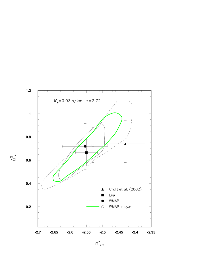
Figure 3: Constraints at $68\%$ CL on the effective slope $n^{*}_{{\rm eff}}$ and power variance $\Delta^{2}_{*}$ at $k^{*}_{p}$=0.03 s/km and $z=2.72$ from: Ly-$\alpha$ cumulative mass function analysis (thin solid contour and filled square), WMAP anisotropy measurements (dashed contour and filled circle) and the joint WMAP and Ly-$\alpha$ analysis (thick solid – green – contour and open circle). See also the discussion in Sect. 3.2. The similar values obtained by Croft et al. 2002 (filled triangle) are also indicated.

Figure 4: The best fit linear power spectrum $P_{L}(k)$ at $z=2.72$ obtained at 68% CL from the analysis of the Ly-$\alpha$ cumulative mass function (open circles and solid line) compared with the transmission power spectrum $P_{F}(k)$ from Croft et al. 2002 (filled circle).

3.2 Combined CMB and Ly-$\alpha$ analysis

By jointly considering the WMAP anisotropy data and the Ly-$\alpha$ observations, we investigate the cosmological constraints obtained on the basis of the analysis of the Ly-$\alpha$ cumulative mass function. To this purpose, we use here only the accurate WMAP temperature anisotropy (TT) power spectrum. In fact, although crucial to probe the cosmological reionization, the inclusion of the polarization (ET) power spectrum derived from WMAP [see also the DASI detection/upper limit on (E and B) polarization power spectrum; Kovac et al. 2002] does not change significantly our quantitative results, as we have verified for a representative set of cases. We will take into account the polarization information in future works. We ran the CMBFAST code v4.2 with the COBE normalization option to generate the CMB temperature anisotropy power spectra for the considered grid of parameters and then renormalized each computed power spectra, $C_{\ell}$, of the grid to minimize the $\chi^{2}$ when compared to the WMAP data (we find that this renormalization does not change appreciably the final best fit and error bar results). We vary $n_{s}$, $w$ and $z_{r}$ in the same range as in the previous analysis, but for this case we also allow to vary the effective running of the slope $dn_{s}/d{\rm ln}k|_{k_{p}}$ at $k_{p}=0.05$Mpc^-1, the same pivot wavenumber used in the analysis by the WMAP team (Spergel et al. 2003).
Our parameter vector has also four dimensions: ${\bf p}=(n_{s},w,z_{r},dn_{s}/d{\rm ln}k$), where $dn_{s}/d{\rm ln}k$ was free to vary in the range $[-0.1,0.1]$ with a step of 0.01. We compute the $\chi^{2}$ for each choice of the parameters in the grid, comparing the simulated CMB temperature anisotropy power spectra with the WMAP anisotropy power spectrum, following the same procedure as in the previous analysis. In addition, for each choice of parameters in the grid we generate the matter transfer function and evaluate the linear matter power spectrum $P_{L}(k)$ at the present time with the normalization given by the equation (22). For each $P_{L}(k)$ we compute the effective slope $n_{{\rm eff}}(k_{p})$ and the running of the slope $dn_{\rm eff}/d{\rm ln}k$ at the pivot wavenumber $k_{p}=0.05$Mpc^-1, as given by equations (24)–(26) by only replacing $k^{*}_{p}$ with $k_{p}$. Note the difference between the two definitions of the running of the slope: $dn_{s}/d{\rm ln}k$ is the matter power law free parameter (see Spergel et al. 2003 and the CMBFAST code v4.2) while $dn_{\rm eff}/d{\rm ln}k$ is obtained from the matter transfer function shape.

Table 2: Cosmological constraints from the joint WMAP and Ly-$\alpha$ analysis. The values of $n_{{\rm eff}}$, $dn_{s}/d\,{\rm ln}k$ and $dn_{\rm eff}/d\,{\rm ln}k$ are evaluated at the pivot wavenumber $k_{p}$=0.05Mpc^-1; $T_{r,4}$ is the reionization temperature in units of $10^{4}$K.

	WMAP+Ly-$\alpha$
Parameter	$68\%$ CL	$95\%$ CL
$n_{s}$	1.034$\pm$0.043	1.011$\pm$0.059
$T_{r,4}$	2.320$\pm$0.194	2.228$\pm$0.229
$z_{r}$	26.131$\pm$3.105	25.495$\pm$3.728
$w$	$-$0.804$\pm$0.122	$-$0.831$\pm$0.115
$\sigma_{8}$	0.945$\pm$0.035	0.949$\pm$0.032
$\tau^{a}$	0.167$\pm$0.028	0.159$\pm$0.032
$\sigma_{8}e^{-\tau}$	0.800$\pm$0.037	0.810$\pm$0.040
$n_{{\rm eff}}$	$-$2.151$\pm$0.045	$-$2.154$\pm$0.047
$dn_{\rm eff}/d\,{\rm ln}k$	0.018$\pm$0.004	0.017$\pm$0.005
$dn_{s}/d\,{\rm ln}k$	0.023$\pm$0.022	0.024$\pm$0.023
aAssumes ionization fraction, $x_{e}$=1.

Figure 5: Panel a): constraints in $n_{{\rm eff}}$ - $dn_{s}/d{\rm ln}k$ plane from MCMC with $dn_{s}/d{\rm ln}k\neq 0$. Panels b) and c): constraints in $n_{{\rm eff}}$ – $\sigma_{8}e^{-\tau}$ plane and $\sigma_{8}e^{-\tau}$ - $dn_{{\rm eff}}/d{\rm ln}k$ plane from MCMC with $dn_{\rm eff}/d{\rm ln}k=0$. All contours and error bars are at $68\%$ CL; $n_{{\rm eff}}$, $dn_{s}/d{\rm ln}k$ and $dn_{\rm eff}/d{\rm ln}k$ are obtained at $k_{p}=0.05$Mpc^-1.

We generate Monte Carlo Markov Chains (MCMC) using the combined $\chi^{2}$ obtained from the Ly-$\alpha$ cumulative mass function and WMAP anisotropy analysis (the number of model elements is of about $3\times 10^{6}$). In this way we sample the chi-squared probability distribution in the combined parameter space. We run the MCMC with $dn_{s}/d{\rm ln}k=0$ and varying $dn_{s}/d{\rm ln}k$ in the range mentioned above.
Before of discussing the results obtained by using the pivot wavenumber $k_{p}$=0.05Mpc^-1 we briefly report on the results we derived by using the pivot point $k^{*}_{p}$=0.03 s/km as in Sect. 3.1 but by exploiting only the WMAP (TT) power spectrum or WMAP combined to the Ly-$\alpha$ information. They are shown again in Figure 3: note how for this pivot point choice the poor sensitivity of WMAP at the small scales accessible to Ly-$\alpha$ observations does not improve but slightly worses the parameter recovery, the two kinds of observations having similar degeneracy directions in the $n^{*}_{\rm eff}-\Delta^{2}_{*}$ plane. On the contrary, the situation improves by considering a pivot wavenumber (namely at $k_{p}$=0.05Mpc^-1) at larger scales. We report in Table 2 the results obtained from the joint WMAP and Ly-$\alpha$ analysis from the MCMC with $dn_{s}/d{\rm ln}k\neq 0$ that can be compared with the WMAP results (Spergel et al. 2003; Peiris et al. 2003).
Panel a) in Figure 5 presents the constraints in $n_{\rm eff}$ - $dn_{s}/d{\rm ln}k$ plane obtained from the analysis of the WMAP anisotropy measurements and the joint WMAP and Ly-$\alpha$ analysis from MCMC with $dn_{s}/d{\rm ln}k\neq 0$. We found that both analyses favour a positive running of the slope $dn_{s}/d{\rm ln}k\approx 0.023$ and an effective spectral index $n_{eff}\approx-2.2$ at $k_{p}$=0.05 Mpc^-1.
Panels b) and c) present the constraints in the $n_{{\rm eff}}$ – $\sigma_{8}e^{-\tau}$ plane and $\sigma_{8}e^{-\tau}$ – $dn_{\rm eff}/d{\rm ln}k$ plane obtained from MCMC with $dn_{s}/d{\rm ln}k=0$ . From the Monte Carlo Markov chain with $dn_{s}/d{\rm ln}k=0$ we found $n_{{\rm eff}}\approx-2.19$ and $dn_{{\rm eff}}/d{\rm ln}k\approx 0.01$.

Our results differ from the value of the effective running of the slope $dn_{s}/d{ln}k\approx-0.03$ found by the WMAP team (Spergel et al. 2003; Peiris et al. 2003) at the same pivot wavenumber and indicate that a possible identification of a running of the slope, $dn_{s}/d{\rm ln}k\neq 0$, at $k_{p}$=0.05Mpc^-1 (multipole ${\it l}\approx 700$) with the current data is mainly an effect of the existing degeneracy in the amplitude-slope plane at this scale, the result being clearly consistent with the absence of running.

In Figure 6 we compare the cosmological parameter constraints at $68\%$ CL from the Ly-$\alpha$ analysis and the joint WMAP and Ly-$\alpha$ analysis with the cosmological parameter “simulated” constraints on cosmological parameters achievable by WMAP after 4 years of observations and by the combination of the three “cosmological” channels of Planck (Mandolesi et al. 1998, Puget et al. 1998, Tauber 2000) at 70, 100, and 143 GHz considering only the multipoles $\ell\leq 1500$ and neglecting the Galactic and extragalactic foreground contamination. We assume Gaussian symmetric beams with the nominal resolution, a sky coverage of $80\%$, the cosmic variance and nominal noise sensitivity as sources of error, and neglect for simplicity possible systematic effects. Only the information from the temperature (TT) power spectrum is again considered. In the case of the “simulated” data we assume exactly the current WMAP data and error bars at $\ell\,\lower 2.0pt\hbox{${<\atop\hbox{\raise 4.0pt\hbox{$\sim$}}}$}\,300$, being the uncertainty in that multipole range dominated by the cosmic variance. We consider as fiducial model the best fit power law $\Lambda$CDM model to the WMAP data with $dn_{s}/d\,{\rm ln}k=0$ (Table 1 from Spergel at al. 2003).

Note the improvement on power spectrum and reionization parameters achievable by using the final WMAP data (improvement of about a factor of two) and that (of about a further factor of two) achievable with Planck by using only the temperature anisotropy data. Note also the role of Planck in reducing the error bar for the parameter $w$ defining the equation of state of the dark energy component parameter.

We find that adding the current Ly-$\alpha$ information to the simulated WMAP 4-yr data only slightly reduces the error bars (of course, the relative improvement is significantly smaller by adding them to the simulated Planck data).

Figure 6: Cosmological parameter constraints at $68\%$ CL from the Ly-$\alpha$ and WMAP+Ly-$\alpha$ analysis compared with the cosmological parameter constraints achievable by WMAP after 4 years of observations and by Planck. For all panels the meaning of the symbols is the same as in panel a). See also the text.

4 Discussion and conclusions

The recent detection of high values of the electron optical depth to the last scattering (Kogut et al. 2003, Spergel et al. 2003) by the WMAP satellite (Bennett et al. 2003) implies the existence of an early epoch of reionization of the Universe at $z_{r}\sim 20$, fundamentally important for understanding the formation and evolution of the structures in the Universe.
As the reionization is assumed to be caused by the ionizing photons produced during the early stages of star-forming galaxies and quasars, we evaluate this effect by computing the cumulative mass function of the high-z bound objects for a class of flat cosmological models with cold dark matter plus cosmological constant or dark energy with constant equation of state, encompassing different reionization scenarios. Our fiducial cosmological model has $\Omega_{b}h^{2}=0.024\pm 0.001$, $\Omega_{m}h^{2}=0.14\pm 0.02$, $h=0.72\pm 0.05$ as indicated by the best fit power law $\Lambda$CDM model of WMAP data (Spergel et al. 2003).

Assuming that the virilization takes place at the collapse time and a constant baryon/dark matter ratio in collapsed objects, we compute the fraction of the mass residing in gravitationally bounded systems as a function of the redshift of collapse at each linear scale and of the virial mass-temperature relation. We evaluate the formation rate of bound objects at $z=2.72$ and their cumulative mass function was compared with the cumulative mass function obtained from the Ly-$\alpha$ transmission power spectrum (Croft et al. 2002).
Our method allows to study reionization models by varying the amplitude, spectrum, and epoch of the reionization and the cosmological parameters. In the same time, as the high-z bound objects are rare fluctuations of the overdensity field, the tail of the cumulative mass function is sensitive to the rms mass fluctuations within the filtering scale $\sigma(R_{f},z)$.
We find that the analysis of the cumulative mass function of the Ly-$\alpha$ systems indicates a reionization redshift in agreement with the value found on the basis of the WMAP anisotropy measurements, setting constraints on the amplitude of the power spectrum, $\sigma_{8}$, similar to those derived from the X-ray cluster temperature function.

Our joint analysis of Ly-$\alpha$ cumulative mass function and WMAP anisotropy measurements shows that a possible identification of a running of the slope, $dn_{s}/d{\rm ln}k\neq 0$, at $k_{p}$=0.05Mpc^-1 (multipole ${\it l}\approx 700$) is mainly an effect of the existing degeneracy in the amplitude-slope plane at this scale, the result being clearly consistent with the absence of running, the other constraints based on WMAP remaining substantially unchanged.

We also shown that, for the set of cosmological models studied in this work, the error bars on the considered parameters can be reduced by about a factor of two by using the final WMAP data. The temperature anisotropy data from the forthcoming Planck satellite will further improve the sensitivity on these parameters, by another factor of two, and also the reliability of these results thanks to the better foreground subtraction achievable with the wider frequency coverage and the improved sensitivity, resolution and systematic effect control. This information jointed with the great improvement on the study of the Ly-$\alpha$ forest trasmission power spectrum (Seljak et al. 2002) achievable by the increase of the number of quasar spectrum measures expected from the Sloan Digital Sky Survey will allow to significantly better constrain the properties of the primordial density field at small scales.

5 Acknowledgements

We acknowledge the use of the computing system at Planck-LFI Data Processing Center in Trieste and the staff working there. LAP acknowledge the financial support from the European Space Agency. It is a pleasure to thank to U. Seljak and M. Zaldarriaga for the use of the CMBFAST code v4.2 employed in the computation of the CMB power spectra and the matter transfer functions.

References

- [1] \harvarditemBecker et al. 2001Becker2001 Becker, R.H. et al. 2001, ApJ, 122, 2850
- [2] \harvarditemBennett et al. 2003Bennett2003 Bennett, C.L. et al. 2003, ApJS, 148, 1
- [3] \harvarditemBond et al. 1991Bond1991 Bond, J.R., Cole, S., Efstathiou, G., Kaiser, N. 1991, ApJ, 379, 440
- [4] \harvarditemCarroll et al. 1992Carroll1992 Carroll, S.M., Press, W.H., Turner, E.L. 1992, MNRAS, 282, ARAA, 30, 499
- [5] \harvarditemCen et al. 1994Cen1994 Cen, R. et al. 1994, ApJ, 437, L9
- [6] \harvarditemChiu & Ostriker 2000ChiuOstriker2000 Chiu, A.W. & Ostriker, P.J. 2000, Apj, 534, 507
- [7] \harvarditemChiu al. 2003Chiu2003 Chiu, A.W., Fan, X. & Ostriker, P.J. 2003, astro-ph/0304234
- [8] \harvarditemCroft et al. 1998Croft1998 Croft, R.A.C. et al. 1998, ApJ, 495, 44
- [9] \harvarditemCroft et al. 2002Croft2002 Croft, R.A.C. et al. 2002, ApJ, 581, 20
- [10] \harvarditemEfstathiou & Rees1988EfstathiouRees1988 Efstathiou, G. & Rees, M.J. 1988, MNRAS, 230, 5P
- [11] \harvarditemEke et al. 1996Eke1996 Eke, V.R., Cole, S. & Frenk, C.S. 1996, MNRAS, 282, 363
- [12] \harvarditemFan et al. 2003Fan2003 Fan, X. et al. 2003, ApJ, in press, astro-ph/0301135
- [13] \harvarditemGnedin & Hamilton 2002GnedinHamilton2002 Gnedin, N.Y. & Hamilton, A.J.S. 2002, MNRAS, 334, 107
- [14] \harvarditemHamilton 2001Hamilton2001 Hamilton A.J.S. 2001, MNRAS, 322, 419
- [15] \harvarditemHeath 1997Heath1997 Heath, D.J. 1997, MNRAS, 179, 351
- [16] \harvarditemHernquist et al. 1996Hernquist1996 Hernquist, L., et al. 1996, ApJ, 457, L51
- [17] \harvarditemHoekstra et al. 2002Hoekstra2002 Hoekstra, H. et al. 2002, ApJ, 577, 604
- [18] \harvarditemHui & Gedin 1997HuiGedin1997 Hui, L. & Gedin, N.Y. 1997, MNRAS, 292, 27
- [19] \harvarditemKaiser 1987Kaiser1987 Kaiser, N. 1987, MNRAS, 227, 1
- [20] \harvarditemKashlinsky & Jones 1991KashlinskyJones1991 Kashlinsky, A. & Jones, B.J.T 1991, Nature, 349, 753
- [21] \harvarditemKashlinsky 1998Kashlinsky1998 Kashlinsky, A. 1998, ApJ , 492, 1
- [22] \harvarditemKitayama & Suto 1997KitayamaSuto1997 Kitayama, T. & Suto, Y. 1997, ApJ, 490, 557
- [23] \harvarditemKogut et al. 2003Kogut2003 Kogut, A. et al. 2003, ApJS, 148, 161
- [24] \harvarditemKolb & Turner 1990KolbTurner1990 Kolb, E.W. & Turner, M.S. 1990, The Early Universe, Addison-Wesley Publishing Co.
- [25] \harvarditemKovac et al. 2002Kovac2002 Kovac, J.M. et al. 2002, Nature, 420, 772
- [26] \harvarditemLacey & Cole 1993LaceyCole1993 Lacey, C. & Cole, S. 1993, MNRAS, 262, 627
- [27] \harvarditemLacey & Cole 1994LaceyCole1994 Lacey, C. & Cole, S. 1994, MNRAS, 271, 676
- [28] \harvarditemLahav et al. 1991Lahav1991 Lahav, O., Lilje, P.B., Primack, J.R., Ress, M.J. 1991, MNRAS, 251, 128
- [29] \harvarditemLilje 1992Lilje1992 Lilje, P.B. 1992, ApJ, 386, L33
- [30] \harvarditemLinde 1990Linde1990 Linde, A. 1990, Particle Physics and Inflationary Cosmology, Harwood Academic Publishers
- [31] \harvarditemMandolesi et al.1998Mandolesi1998 Mandolesi, N., et al. 1998, Planck Low Frequency Instrument, A Proposal Submitted to ESA
- [32] \harvarditemMiralda-Escudé et al. 2000MiraldaEscude2000 Miralda-Escudé, J., Haehnelt, M. & Ress, M.J. 2000, ApJ, 530, 1
- [33] \harvarditemMcDonald & Miralda-Escudé1999McDonaldMiraldaEscude1999 McDonald, P. & Miralda-Escudé, J. 1999, ApJ, 518, 24
- [34] \harvarditemMcDonald et al. 2000McDonald2000 McDonald, P. et al. 2000, ApJ, 543, 1
- [35] \harvarditemMonaco 1995Monaco1995 Monaco, P. 1995, ApJ, 447, 23
- [36] \harvarditemPeacock & Dodds 1996PeacockDodds1996 Peacock J.A. & Dodds S.J. 1996, MNRAS, 280, L19
- [37] \harvarditemPeiris et al. 2003Peiris2003 Peiris, H.V. et al. 2003, ApJS, 148, 216
- [38] \harvarditemPuget et al.1998Puget1998 Puget, J.L., et al. 1998, High Frequency Instrument for the Planck Mission, A Proposal Submitted to the ESA
- [39] \harvarditemPress & Schechter 1974PressSchechter1974 Press, W.H. & Schechter, P. 1974, ApJ, 187, 452
- [40] \harvarditemSongaila & Cowie 2002SongailaCowie2002 Songaila, A. & Cowie, L.L. 2002, ApJ, 123, 2183
- [41] \harvarditemSasaki 1994Sasaki1994 Sasaki, S. 1994, PASJ, 46, 427
- [42] \harvarditemSeljak et al. 2002Seljak2002 Seljak, U., Mandelbaum, R. & McDonald, P. 2002, Constraining the dark energy with Ly-alpha forest, to appear in proceedings of the XVIII’th IAP Colloquium, On the Nature of Dark Energy, IAP Paris, astro-ph/0212343
- [43] \harvarditemSeljak et al. 2003Seljak2003 Seljak, U., McDonald, P. & Makarov, A. 2003, MNRAS, 342, L79
- [44] \harvarditemSeljak & Zaldarriaga 1996SeljakZaldarriaga1996 Seljak, U. & Zaldarriaga, M. 1996, ApJ, 469, 437
- [45] \harvarditemSpergel et al. 2003Spergel2003 Spergel, D.N. et al. 2003, ApJS, 148, 175
- [46] \harvarditemTauber2000Tauber2000 Tauber, J.A., 2000, The Planck Mission, in The Extragalactic Infrared Background and its Cosmological Implications, Proceedings of the IAU Symposium, Vol. 204, M. Harwit and M. Hauser, eds.
- [47] \harvarditemTheuns et al. 1998Theuns1998 Theuns, T., et al. 1998, MNRAS, 301, 478
- [48] \harvarditemVerde et al. 2002Verde2002 Verde, L. et al. 2002, MNRAS, 335, 432
- [49] \harvarditemVerde et al. 2003Verde2003 Verde, L. et al. 2003, ApJS, 148, 195
- [50] \harvarditemViana & Liddle 1996VianaLiddle1996 Viana, P.T.P & Liddle, A.R. 1996, MNRAS, 281, 323
- [51] \harvarditemVogt et al. 1994Vogt1994 Vogt, S.S. et al. 1994, Proc. SPIE, 2198, 362
- [52] \harvarditemWang & Steinhardt 1998WangSteinhardt1998 Wang, L. & Steinhardt, P.J. 1998, ApJ, 508, 483
- [53] \harvarditemWhite et al. 2003White2003 White, R.L., Becker, R.H., Fan, X., Strauss, M.A. 2003, AJ, in press, astro-ph/0303476
- [54] \harvarditemZaldarriaga et al. 2003Zaldarriaga2003 Zaldarriaga, M., Scoccimarro, R., Hui, L. 2003, ApJ, 590, 1
- [55] \harvarditemZhang et al. 1995Zhang1995 Zhang, Y., Anninos, P., Norman, M.L. 1995, ApJ, 453, L57
- [56]