A Proposal to Search for Transparent Hidden Matter Using Optical Scintillation

It is proposed to search for scintillation of extragalactic sources through the last unknown baryonic structures. Appropriate observation of the scintillation process described here should allow one to detect column density stochastic variations in cool Galactic molecular clouds of order of $\sim 3\times 10^{-5}\,\mathrm{g/cm^{2}}$ – that is $10^{19}\,\mathrm{molecules/cm^{2}}$ – per $\sim 10\,000\,\mathrm{km}$ transverse distance.

1 Introduction

It has been suggested that a hierarchical structure of cold $\mathrm{H_{2}}$ could fill the Galactic thick disk $\!{}^{{\bf?}}$ or halo $\!{}^{{\bf?}}$, providing a solution for the Galactic dark matter problem. This gas could form undetectable “clumpuscules” of $10\,\mathrm{AU}$ size at the smallest scale, with a column density of $10^{24-25}\,\mathrm{cm^{-2}}$, and a surface filling factor less than 1%. Light propagation is delayed through such a structure and the average transverse gradient of optical path variations is of order of $1\lambda\ per\ 10\,000\,\mathrm{km}$ at $\lambda=500\,\mathrm{nm}$. These $\mathrm{H_{2}}$ clouds could then be detected through their diffraction and refraction effects on the propagation of the light of background stars (for a more detailed paper on this proposal see ( $\!{}^{{\bf?}}$)).

2 Detection mode of extended $\mathrm{H_{2}}$ clouds: principle

Due to index refraction effects, an inhomogeneous transparent medium (hereafter called screen) distorts the wave-fronts of incident electromagnetic waves (see Fig. 2). The extra optical path induced by a screen at distance $z_{0}$ can be described by a phase delay $\delta(x_{1},y_{1})$ in the plane transverse to the observer-source line. The amplitude $A_{0}$ in the observer’s plane results from the subsequent propagation, that is described by the Huygens-Fresnel diffraction theory

$$A_{0}(x_{0},y_{0})=\frac{Ae^{2i\pi z_{0}/\lambda}}{2i\pi R_{F}^{2}}\int\!\!\int_{-\infty}^{+\infty}e^{\frac{2i\pi\delta(x_{1},y_{1})}{\lambda}}e^{i\frac{(x_{0}-x_{1})^{2}+(y_{0}-y_{1})^{2}}{2R_{F}^{2}}}dx_{1}dy_{1},$$ (1)

where $A$ is the incident amplitude (before the screen), taken as a constant for a very distant on-axis source, and $R_{F}=\sqrt{\lambda z_{0}/2\pi}$ is the Fresnel radius. $R_{F}$ is of order of $1500\,\mathrm{km}$ to $15\,000\,\mathrm{km}$ at $\lambda=500\,\mathrm{nm}$, for a screen distance $z_{0}$ between $1\,\mathrm{kpc}$ to $100\,\mathrm{kpc}$. The resulting intensity in the observer’s plane is affected by strong interferences (the so-called speckle) if $\delta(x_{1},y_{1})$ varies stochastically of order of $\lambda$ within the Fresnel radius domain. This is precisely the same order of magnitude as the average gradient that characterizes the hypothetic $\mathrm{H_{2}}$ structures.

As for radio-astronomy $\!{}^{{\bf?}}$^,$\!{}^{{\bf?}}$, the stochastic variations of $\delta(x_{1},y_{1})$ can be characterized by the diffractive length scale $R_{diff}$, defined as the transverse separation for which the root mean square of the optical path difference is $\lambda/2\pi$.

• If $R_{diff}\gg R_{F}$, the screen is weakly diffusive. The wavefront is weakly corrugated, producing weakly contrasted patterns with length scale $R_{F}$ in the observer’s plane (Fig. 2).

• If $R_{diff}\ll R_{F}$, the screen is strongly diffusive. Two modes occur, the diffractive scintillation – producing strongly contrasted patterns characterized by the length scale $R_{diff}$ – and the refractive scintillation – giving less contrasted patterns and characterized by the large scale structures of the screen $R_{ref}$ –.

We focus here on the strong diffractive mode, which should produce the most contrasted patterns and is easily predictable.

3 Basic configurations

Fig. 1 (left) displays the expected intensity variations in the observer’s plane for a point-like monochromatic source observed through a transparent screen with a step of optical path $\delta=\lambda/4$ and through a prism edge. The inter-fringe is – in a natural way – close to the length scale defined by $\sqrt{\pi}R_{F}$.

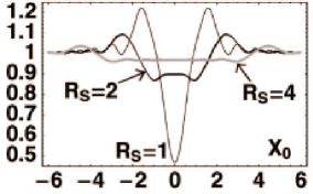
Figure 1: Relative intensity diffraction patterns produced in the observer’s plane, perpendicularly to a width step or prism. From left to right: - Step of optical path $\delta=\lambda/4$ - Prism of optical path with $\delta=X_{0}\times\lambda/2$ for $X_{0}>0$. - Step of optical path $\delta=\lambda/2$, for extended disk-sources of reduced radius $R_{S}=1$, 2 and 4. The $X_{0}-\mathrm{axis}$ origin ($X_{0}=x_{0}/\sqrt{\pi}R_{F}$) is the intercept of the source-step line with the observer’s plane.

Such configurations model the edge of a $\mathrm{H_{2}}$ structure, because they have the same average gradient of optical path. More generally, contrasted patterns take place as soon as the second derivative of the optical path is different from zero.

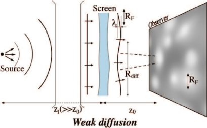
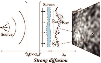
Figure 2: The two scintillation regimes: Left: $R_{diff}\gg R_{F}$. The weakly distorted wavefront produces a weak scintillation at scale $R_{F}$ in the observer’s plane. Right: $R_{diff}\ll R_{F}$. The strongly distorted wavefront produces strong scintillation at scales $R_{diff}$ (diffractive mode) and $R_{ref}$ (refractive mode).

4 Limitations from spatial and temporal coherences

At optical wavelengths, diffraction pattern contrast is severely limited by the size of the source $r_{S}$. Fig. 1 (right) shows the diffraction patterns for different reduced source radii, defined as $R_{S}=r_{s}/(\sqrt{\pi}R_{F})\times z_{0}/z_{1}$, where $z_{1}$ is the distance from the source to the screen.

In return, temporal coherence with the standard UBVRI filters is sufficiently high to enable the formation of contrasted interferences in the configurations considered here. The fringe jamming induced by the wavelength dispersion is also much smaller than the jamming due to the source extension.

5 What is to see?

An interference pattern with inter-fringe of $\sim R_{F}$ ($1000-10\,000\,\mathrm{km}$ at $\lambda=500\,\mathrm{nm}$) is expected to sweep across the Earth when the line of sight of a sufficiently small astrophysical source crosses an inhomogeneous transparent Galactic structure (see Table 1). This pattern moves at the transverse velocity $V_{T}$ of the diffusive screen. Its shape may also evolve, due to random turbulence in the scattering medium. For the Galactic $\mathrm{H_{2}}$ clouds we are interested in, we expect a typical modulation index $m_{scint}$ (or contrast) ranging between 1% and $\sim 20\%$, critically depending on the source apparent size. The time scale $t_{scint}=R_{F}/V_{T}$ of the intensity variations is of order of $30\,\mathrm{s}$. As the inter-fringe scales with $\sqrt{\lambda}$, one expects a significant difference in the time scale $t_{scint}$ between the red side of the optical spectrum and the blue side. This property might be used to sign the diffraction phenomenon at the $R_{F}$ natural scale.

Table 1: Configurations leading to strong diffractive scintillation. Here we assume a regime characterized by $R_{diff}\leq R_{F}$, or at least a transitory regime as described in Section 3 – characterized by $R_{F}$ –, for example if an inhomogeneity due to a turbulent mechanism crosses the line of sight. Numbers are given for $\lambda=500\,\mathrm{nm}$.

		SCREEN
		atmos-	solar	solar	Galactic
		phere	system	suburbs	thin disk	thick disk	halo
Distance		$10\,\mathrm{km}$	$1\,\mathrm{AU}$	$10\,\mathrm{pc}$	$300\,\mathrm{pc}$	$1\,\mathrm{kpc}$	$10\,\mathrm{kpc}$
$R_{F}$ to $\times$ by $\left[\frac{\lambda}{500\,\mathrm{nm}}\right]^{\frac{1}{2}}$		$2.8\,\mathrm{cm}$	$109\,\mathrm{m}$	$157\,\mathrm{km}$	$860\,\mathrm{km}$	$1570\,\mathrm{km}$	$5000\,\mathrm{km}$
Transverse speed $V_{T}$		$1\,\mathrm{m/s}$	$10\,\mathrm{km/s}$	$20\,\mathrm{km/s}$	$30\,\mathrm{km/s}$	$40\,\mathrm{km/s}$	$200\,\mathrm{km/s}$
$t_{scint}$ to $\times\left[\frac{\lambda}{500\,\mathrm{nm}}\right]^{\frac{1}{2}}\left[\frac{R_{diff}}{R_{F}}\right]$		$0.03\,\mathrm{s}$	$0.01\,\mathrm{s}$	$8\,\mathrm{s}$	$29\,\mathrm{s}$	$40\,\mathrm{s}$	$25\,\mathrm{s}$
$m_{scint}$ in % to multiply by			$32\%\times$	$2.2\%\times$	$4.1\%\times$	$2.2\%\times$	$7.1\%\times$
$\left[\frac{\lambda}{500\,\mathrm{nm}}\right]^{\frac{1}{2}}\left[\frac{R_{diff}}{R_{F}}\right]\left[\frac{r_{S}}{r_{\odot}}\right]^{-1}$		$100\%$	$\left[\frac{d}{10\mathrm{pc}}\right]$	$\left[\frac{d}{1\mathrm{kpc}}\right]$	$\left[\frac{d}{10\mathrm{kpc}}\right]$	$\left[\frac{d}{10\mathrm{kpc}}\right]$	$\left[\frac{d}{100\mathrm{kpc}}\right]$
SOURCE		DIFFRACTIVE MODULATION INDEX $m_{scint}$
Location	Type	(to multiply by $\sqrt{\lambda/500\,\mathrm{nm}}\times R_{diff}/R_{F}$)
nearby 10pc	any star	$\ll 1\%$	$<100\%$
Galactic 8kpc	star	in a	100%	1-70%	1-10%
LMC 55kpc	A5V ($r_{S}=1.7r_{\odot}$)	tele-	100%	70%	13%	7%	2%
M31 725kpc	B0V ($r_{S}=7.4r_{\odot}$)	scope	100%	100%	40%	22%	7%
z=0.2–0.9Gpc	SNIa	$>1\,\mathrm{m}$	100%	70%	13%	7%	2%
z=1.7–1.7Gpc	Q2237+0305		100%	$>45\%$	$>8\%$	$>4\%$	$>1.4\%$

6 How to see it?

Minimal hardware: from Table 1, we deduce that the minimal magnitude of extragalactic stars that are likely to undergo a few percent modulation index from a Galactic molecular cloud is $M_{V}\sim 20.5$ (A5V star in LMC or B0V in M31). Therefore, the search for diffractive scintillation needs the capability to sample every $\sim 10\,\mathrm{s}$ (or faster) the luminosity of stars with $M_{V}>20.5$, with a point-to-point precision better than a few percent. This performance can be achieved using a 2 meter telescope with a high quantum efficiency detector allowing a negligible dead time between exposures (like frame-transfer CCDs). Multi-wavelength detection capability is highly desirable to exploit the dependence of the diffractive scintillation pattern with the wavelength.

Chances to see something? The $1\%$ surface filling factor predicted for gaseous structures is also the maximum optical depth for all the possible refractive (weak or strong) and diffractive scintillation regimes. Under the pessimistic hypothesis that strong diffractive regime occurs only when a Galactic structure enters or leaves the line of sight, the duration for this regime is of order of $\sim 5$ minutes (time to cross a few fringes) over a total typical crossing time of $\sim 400$ days. Then the diffractive regime optical depth $\tau_{scint}$ should be at least of order of $10^{-7}$ and the average exposure needed to observe one event of $\sim 5$ minute duration is $10^{6}\,\mathrm{star\times hr}$ . It follows that a wide field detector is necessary to monitor a large number of stars.

7 Foreground effects, background to the signal

Atmospheric effects: Surprisingly, atmospheric intensity scintillation is negligible through a large telescope ($m_{scint}\ll 1\%$ for a $>1\,$m diameter telescope $\!{}^{{\bf?}}$). Any other long time scale atmospheric effect such as absorption variations at the sub-minute scale (due to fast cirruses for example) should be easy to recognize as long as nearby stars are monitored together.

The solar neighbourhood: Overdensities at $10\,\mathrm{pc}$ could produce a signal very similar to one expected from the Galactic clouds. But in this case, even big stars should undergo a contrasted diffractive scintillation; the distinctive feature of scintillation through more distant screens ($>300\,\mathrm{pc}$) is that only the smallest stars are expected to scintillate. It follows that simultaneous monitoring of various types of stars at various distances should allow one to discriminate effects due to solar neighbourhood gas and due to more distant gaseous structures.

Sources of background? Physical processes such as asterosismology, granularity of the stellar surface, spots or eruptions produce variations of very different amplitudes and time scales. A few categories of recurrent variable stars exhibit important emission variations at the minute time scale $\!{}^{{\bf?}}$, but their types are easy to identify from spectrum.

8 Conclusions and perspectives

Structuration of matter is perceptible at all scales, and the eventuality of stochastic fluctuations producing diffractive scintillation is not rejected by observations. In this paper, I showed that there is an observational opportunity resulting from the subtle compromise between the arm-lever of interference patterns due to hypothetic diffusive objects in the Milky-Way and the size of the extra-galactic stars. The hardware and software techniques required for scintillation searches are currently available. Tests are under way to validate some of the ideas discussed here.

If some indications are discovered with a single telescope, one will have to consider a project involving a 2D array of telescopes, a few hundred and/or thousand kilometers apart. Such a setup would allow to temporally and spatially sample an interference pattern, unambiguously providing the diffraction length scale $R_{diff}$, the speed and the dynamics of the scattering medium.

References

References

- [1] D. Pfenniger & F. Combes A&A 285, 94 (1994).
- [2] F. De Paolis et al. Phys. Rev. Lett. 74, 14 (1995).
- [3] M. Moniez, to appear in A&A, astro-ph/0302460, LAL-report 03-34 (2003).
- [4] A.G. Lyne & F. Graham-Smith, Pulsar Astronomy, Cambridge University Press (1998).
- [5] R. Narayan Phil. Trans. R. Soc. Lond. A 341, 151 (1992).
- [6] D. Dravins et al. Pub. of the Ast. Soc. of the Pacific 109 (I, II) (1997), 110 (III) (1998).
- [7] C. Sterken & C. Jaschek light Curves of Variable Stars, a pictorial Atlas, Cambridge University Press (1996).