Quantifying the bimodal color-magnitude distribution of galaxies

Abstract

We analyse the bivariate distribution, in color versus absolute magnitude ($u-r$ vs. $M_{r}$), of a low redshift sample of galaxies from the Sloan Digital Sky Survey (SDSS; 2400 deg², $0.004<z<0.08$, $-23.5<M_{r}<-15.5$). We trace the bimodality of the distribution from luminous to faint galaxies by fitting double-Gaussians to the color functions separated in absolute magnitude bins. Color-magnitude (CM) relations are obtained for red and blue distributions (early- and late-type, predominantly field, galaxies) without using any cut in morphology. Instead, the analysis is based on the assumption of normal Gaussian distributions in color. We find that the CM relations are well fit by a straight line plus a tanh function. Both relations can be described by a shallow CM trend (slopes of about $-0.04$, $-0.05$) plus a steeper transition in the average galaxy properties over about two magnitudes. The midpoints of the transitions ($M_{r}=-19.8$ and $-20.8$ for the red and blue distributions, respectively) occur around $2\times 10^{10}$ ${\cal M}_{\odot}$ after converting luminosities to stellar mass. Separate luminosity functions are obtained for the two distributions. The red distribution has a more luminous characteristic magnitude and a shallower faint-end slope ($M^{*}=-21.5$, $\alpha=-0.8$) compared to the blue distribution ($\alpha\approx-1.3$ depending on the parameterization). These are approximately converted to galaxy stellar mass functions. The red distribution galaxies have a higher number density per magnitude for masses greater than about $3\times 10^{10}$ ${\cal M}_{\odot}$. Using a simple merger model, we show that the differences between the two functions are consistent with the red distribution being formed from major galaxy mergers.

1. Introduction

Optical color-magnitude (CM) diagrams have been used as scientific diagnostics in astronomy since the pioneering work of E. Hertzsprung and H. N. Russell (c. 1910). While the CM relations for stars are now well established in terms of stellar evolution theory, the case for galaxies is less clear. The optical spectra of galaxies are dominated by the integrated light from stellar populations, and therefore, the existence of any CM sequence is related to a correlation of galaxy luminosity with star-formation history (SFH), stellar initial mass function (IMF), chemical evolution and/or dust attenuation. In order to separate CM relations from color-morphology relations, most of the study of CM relations has concerned galaxies of a similar morphological type. The principal relationship between color and morphology (Holmberg, 1958; Roberts & Haynes, 1994) is that more spheroidal-like galaxies (early types) are generally redder than more disk-like or irregular galaxies (late types).

A color-magnitude relation for spheroidal-like systems was first established by Baum (1959). The integrated colors become systematically redder going from globular star clusters, through dwarf elliptical galaxies, to giant ellipticals. Later, more precise measurements of luminous E+S0 galaxies in clusters showed a shallow CM relation with a small intrinsic scatter (Faber, 1973; Visvanathan & Sandage, 1977). This relation was associated with a metallicity-luminosity correlation (Faber, 1973; Larson, 1974). However, Worthey, Trager, & Faber (1995) showed that a age-luminosity correlation also fit the spectroscopic data because of the age-metallicity degeneracy. Kodama & Arimoto (1997) ruled out the correlation with age being the primary effect because the predicted evolution of the CM sequence with redshift was more than observed in this case. Thus, the CM relation for bright E+S0 galaxies has been established as a metallicity-luminosity correlation. The intrinsic scatter and slope of this ‘E+S0 ridge’ can be used to place constraints on the star-formation and merging histories of these galaxies (Bower, Kodama, & Terlevich, 1998).

Color-magnitude relations for early-type spirals were established by Visvanathan & Griersmith (1977) and for spirals in general by Chester & Roberts (1964); Visvanathan (1981); Tully, Mould, & Aaronson (1982). These CM relations are more complicated than for the E+S0 ridge for a number of reasons. The intrinsic is scatter is larger (Griersmith, 1980) and the luminosity correlations can be associated with SFH (Peletier & de Grijs, 1998), dust attenuation (Tully et al., 1998) and/or metallicity (Zaritsky, Kennicutt, & Huchra, 1994). It is probable that for some morphological types and across some ranges of absolute magnitude, all three effects are significant.

When all morphological types are considered together, the color distribution of galaxies can be approximated by the sum of two ‘normal’ Gaussian functions, a bimodal function (Strateva et al., 2001). The bimodality of the galaxy population has been known qualitatively for some time. Researchers general consider E+S0 galaxies to be early types and Sa-Sd spirals and irregulars to be late types, and Tully et al. (1982) noted that “early and late morphological types occupy separate branches in the color-magnitude diagram”. With the advent of large spectroscopic redshift surveys, it is now possible to precisely analyse this color bimodality as a function of absolute magnitude, for the field population in particular (whereas previously clusters offered the best opportunity to study CM relations since all the cluster members are approximately at the same distance).

A natural explanation for the bimodality is that the two normal distributions represent different populations of galaxies that are produced by two different sets of processes. In other words, formation processes give rise to two dominant populations that have different average colors and/or color dispersions. Evidence that the color bimodality is due to this comes from the clustering analysis of Budavari et al. (2003). When the galaxy population was divided into four color bins, the two reddest bins showed a similar clustering strength to each other, as did the two bluest bins, with a sharp transition in properties between them. This can be explained if the dominant effect is the fraction of galaxies that are part of the red or blue normal distributions, rather than the average color of the galaxies. Galaxies that are part of the red distribution are more strongly clustered.

Bell et al. (2003b) used only colors to define a red sequence from a photometric redshift survey. The bimodality was observed out to a redshift of unity and the evolution of the red sequence was quantified. In particular, they noted a build up of stellar mass on the red sequence by a factor of about two since $z=1$. This is inconsistent with a scenario where red early-type galaxies form early in the Universe and evolve passively to the present day, and it favors scenarios where the red sequence derives from merger processes.

For our color analysis, we use data from the Sloan Digital Sky Survey (SDSS). The SDSS is unique for studying the CM distribution of low-redshift galaxies because the survey has obtained over $10^{5}$ redshifts for $z<0.1$ galaxies with associated five-color photometry. An overview of various bivariate distributions, including CM relations, is given by Blanton et al. (2003c). Here, we focus on one particular color and analyse in more detail the low-redshift distribution of galaxies ($z<0.08$; $u-r$ vs. $M_{r}$). We also extract luminosity functions for the red and blue distributions (early- and late-type galaxies), relate our results to stellar mass and consider a merger explanation for the bimodality. The plan of the paper is as follows; in Section 2, we describe the SDSS data and sample selection; in Section 3, we show the CM bivariate distribution; in Section 4, we describe our assumptions, aims and the parametric analysis of the distribution, and; in Sections 5 and 6, we present our results and conclusions. A simple merger model is described in the Appendix.

2. The SDSS Data and Sample Selection

The Sloan Digital Sky Survey (York et al., 2000; Stoughton et al., 2002) is a project, with a dedicated 2.5-m telescope, designed to image $10^{4}$ deg² and obtain spectra of $10^{6}$ objects. The imaging covers five broadbands, $ugriz$ with effective wavelengths of 355, 467, 616, 747 and 892 nm, using a mosaic CCD camera (Gunn et al., 1998). Observations with a 0.5-m photometric telescope (Hogg et al., 2001) are used to calibrate the 2.5-m telescope images using the $u^{\prime}g^{\prime}r^{\prime}i^{\prime}z^{\prime}$ standard star system (Fukugita et al., 1996; Smith et al., 2002). Spectra are obtained using a 640-fiber fed spectrograph with a wavelength range of 380 to 920 nm and a resolution of $\lambda/\Delta\lambda\sim 1800$ (Uomoto et al., 1999). In this paper, we analyse a sample of galaxies selected from the SDSS main galaxy sample (MGS; Strauss et al., 2002) that selects objects for spectroscopic followup to a limiting magnitude in the $r$-band.

The imaging data are astrometrically calibrated (Pier et al., 2003) and the images are reduced using a pipeline photo that measures the observing conditions, and detects and measures objects. In particular, photo produces various types of magnitude measurement including: (i) ‘Petrosian’, the summed flux in an aperture that depends on the surface-brightness profile of the object, a modified version of the flux quantity defined by Petrosian (1976); (ii) ‘model’, a fit to the flux using the best fit of a de-Vaucouleurs and an exponential profile; (iii) ‘PSF’, a fit using the local point-spread function. The magnitudes are extinction-corrected using the dust maps of Schlegel, Finkbeiner, & Davis (1998). Details of the imaging pipelines are given by Lupton et al. (2001) and Stoughton et al. (2002).

Once a sufficiently large area of sky has been imaged, the data are analysed using ‘targeting’ software routines that determine the objects to be observed spectroscopically. The MGS has the following basic criteria:

$$r_{\rm Petro} < r_{\rm limit}$$ (1)

$$\mu_{r,{\rm 50}} < \mu_{r,{\rm 50,limit}}$$ (2)

$$r_{\rm PSF}-r_{\rm model} > s_{\rm limit}\>.$$ (3)

The first equation sets the magnitude limit of the survey. The second equation sets the surface-brightness limit ($\mu_{r,{\rm 50}}$ is the mean surface brightness within the Petrosian half-light radius). This is necessary to avoid targeting too many objects that are instrumental artifacts. The third equation is used for star-galaxy separation. The limits have been modified since the beginning of the survey but over most of the survey, they are given by $r_{\rm limit}=17.77$, $\mu_{r,{\rm 50,limit}}=24.5$ mag arcsec^-2 and $s_{\rm limit}=0.3$. The targets from all the samples (others include luminous red galaxies and quasars) are then assigned to plates, each with 640 fibers, using a tiling algorithm (Blanton et al., 2003a). Details of the MGS selection are given by Strauss et al. (2002).

Spectra are taken using, typically, three 15-minute exposures in moderate conditions (the best conditions are used for imaging). The signal-to-noise ratio (S/N) is typically 10 per pixel (pixels width $\approx 1$–2Å) for galaxies in the MGS. The pipeline spec2d extracts, and flux and wavelength calibrates, the spectra. The spectra are then analysed by another pipeline that classifies and determines the redshift of the object.

2.1. Subsample Selection from the Main Galaxy Sample

We use a well-defined subsample of the MGS called ‘NYU LSS sample12’ covering 2400 deg². We set limits on the magnitude as follows: $13.5<r<17.5$ over 30% and $13.5<r<17.77$ over 70% of the area. The 17.5-limit corresponds to earlier targeting when the imaging and targeting pipelines were significantly different from the 17.77-limit. This produces a sample of 207654 objects, of which, 94% have been observed spectroscopically. The remaining 6% are primarily missed due to ‘fiber collisions’, which means that the tiling pipeline is unable to assign fibers due to another target being less than 55” away. This is a limit imposed by the plate and fiber technology. When two or more MGS targets are within 55” of each other, a fiber is assigned at random to one of them. Of the spectroscopically observed targets, 99.5% have reliable redshifts determined and, of these, 97.7% are galaxies with redshifts between 0.001 and 0.3.

We further restrict our sample to a low redshift range of $0.004<z<0.080$ and a range in absolute magnitude of $-23.5<M_{r}<-15.5$, given by

$$M_{r}=r-k_{r}-5\log(D_{L}/{\rm\,10\,pc})$$ (4)

where: $r$ is the Milky-Way extinction-corrected, Petrosian magnitude; $D_{L}$ is the luminosity distance for a cosmology with $(\Omega_{m},\Omega_{\Lambda})_{0}$ = (0.3,0.7) and $H_{0}=(h_{70}){\rm\,70\,km\,s^{-1}\,Mpc^{-1}}$, and; $k_{r}$ is the k-correction using the method of Blanton et al. (2003b). This produces a sample of 66846 galaxies with reliable redshift measurements.

Including higher redshift galaxies can leverage better statistics on the bright galaxies but here we are also interested in the continuity between low and high luminosity galaxies. In addition, restricting the sample to $z<0.08$, reduces evolution effects and uncertainties in $k$-corrections. Blanton et al. (2003c) reduced these types of uncertainties by $k$-correcting to the $z=0.1$ bandpasses. This is optimal for the median redshift galaxies in the MGS but is sub-optimal for low luminosity galaxies (only observed near $z=0$). Therefore, we keep to the standard definition of $k$-corrections (to $z=0$). This also means that no extrapolation is required to get from the observed-frame bandpasses to the rest-frame $u$ and $r$ bands principally used in our analysis.

3. The Bivariate Distribution

For a spectral-type indicator, we use the rest-frame $u-r$ color defined by

$$C_{ur}=(u_{\rm model}-k_{u})-(r_{\rm model}-k_{r})\>.$$ (5)

This is used because, even without $k$-corrections, the $u-r$ color has been shown to be a nearly optimal separator into two color types (Strateva et al., 2001). The $u$-band filter observes flux from below the 4000Å break and thus any $u-X$ color is highly sensitive to SFH ($X=g,r,i$ or $z$). We determined that using $u-r$ gave the most robust results for the analysis presented in this paper (though $u-g$ gave a marginally better division by type for the more luminous galaxies).

Model magnitudes are used because they give a higher S/N measurement than the Petrosian magnitudes, particularly because the $u$-band flux is generally weak and aperture photometry includes significant Poisson and background-subtraction uncertainties. In fact, if Petrosian colors are used, using the $u$-band may not be optimum. For example, Blanton et al. (2003c) found that the bimodality was most evident in the ${}^{0.1}(g-r)$ color. Note that SDSS model magnitudes are determined using the best-fit profile obtained from the $r$-band image and fitting only the amplitude in the other bands.

The bivariate distribution of the sample in $C_{ur}$ versus $M_{r}$ is shown in Figure 1. The bimodality is clearly visible with two tilted ridges representing the early- and late-type galaxies. The other $u-X$ CM distributions appear similar (after scaling the color-axis appropriately). For the $g-X$ CM distributions, the bimodality is still evident (at low luminosities) but the late-type ridge appears to merge with the early-type ridge around $M_{r}\sim-20$ whereas this occurs at slightly higher luminosities with the $u-X$ colors. This probably reflects the changing dependence of dust and SFH on the colors of the late-type galaxies. For the remaining CM distributions ($r-i$, $r-z$, $i-z$), the bimodality is not evident as the ridges have merged.

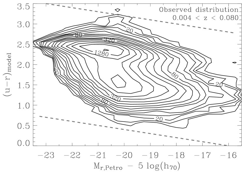
Figure 1.— Observed bivariate distribution of the sample in rest-frame color versus absolute magnitude. The contours are determined for galaxy number counts in 0.1 color $\times$ 0.5 magnitude bins (with a total of 66846 galaxies). The contour levels are on a logarithmic scale, starting at 10 and doubling every two contours. The dashed lines represent the limits used in the double-Gaussian fitting described in Section 4.

3.1. Correcting for Incompleteness

Before the distribution is analysed, there are two significant incompleteness issues to deal with: (i) galaxies of a given absolute magnitude and spectral type can only be observed within a certain redshift range, which in some cases is much less than the redshift range of the sample, and; (ii) some galaxies are not observed due to fiber collisions.

To correct for the first issue, we weight each galaxy by a $V_{\rm survey}/V_{\rm max}$ factor before recomputing the bivariate distribution, where $V_{\rm max}$ is the maximum volume over which the galaxy could be observed within the sample redshift range ($0.004<z<0.08$, $V_{\rm survey}=9.3\times 10^{6}\,{\rm Mpc}^{3}$). We calculate $V_{\rm max}$ by iterating to a solution for the $k$-correction at $z_{\rm min}$ and $z_{\rm max}$. The factor, $V_{\rm survey}/V_{\rm max}$, varies from about 1.4 for the brightest galaxies (set by $r>13.5$), down to 1.01 at $M_{r}\approx-21$, up to 450/650 for the faintest galaxies (set by $r<17.5$/17.77). In the 17.77-limit region, the sample is virtually volume limited between absolute magnitudes of $-23$ and $-20$ ($V_{\rm survey}/V_{\rm max}$$\lesssim 1.2$). Note also that this correction factor is principally a function of $M_{r}$ with little dependence on color at these low redshifts ($r$-selected sample), which means that this correction is important for the determination of the luminosity functions but not for the CM relations.

The class of galaxies that are not observed due to fiber collisions is not identical to the whole sample. On average, these galaxies will be found in higher density regions. A very similar class of galaxies are those that are the nearest observed neighbors to the unobserved galaxies. These galaxies were, predominantly by chance, allocated a fiber instead of their neighbors. To correct for this issue, we weight these observed galaxies by 2.15. This factor is determined from the number of unobserved galaxies divided by the number of unique nearest observed neighbors, plus unity.

The corrected distribution of galaxies is shown in Figure 2. The results of our fitting to the mean color values along the red and blue distributions are also shown (described later). In the next section, we describe our parametric fitting to the bimodal bivariate distribution.

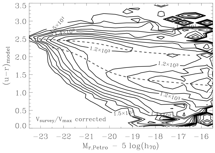
Figure 2.— Bivariate distribution of the sample in rest-frame color versus absolute magnitude, $V_{\rm survey}/V_{\rm max}$ corrected. The contours are determined for galaxy number counts in 0.1 color $\times$ 0.5 magnitude bins. The contour levels are on a logarithmic scale, starting at 15 and trebling every two contours. The upper and lower dashed lines represent a fit to the mean positions of the Gaussian color functions for the red and blue distributions, respectively (the fitting is described in Sec. 4, see also Fig. 6).

4. Methodology

First of all, we summarize our assumptions and aims before describing our parameterization and fitting procedure. Our basic assumptions are given below.

1. There are two dominant sets of processes that lead to two distributions of galaxies.

2. For each distribution, the average spectral properties vary contiguously with visible luminosity. This is reasonable because luminosity is correlated with the mass of a galaxy and gravity determines the movement of gas and stars.

3. At each luminosity, each distribution can be approximated using a normal distribution in the difference between the near-ultraviolet and visible magnitudes (a log-normal distribution in the ratio between the fluxes). This could result from stochastic variations in SFH, metallicity and dust content (and inclination in the case of disks).

Note that for our discussion, we assume that the stellar IMF is universal (Wyse, 1997; Kroupa, 2002).

Our aims are:

1. to quantitatively determine the variation in the mean and dispersion of the spectral colors of each distribution, as a function of luminosity;

2. to determine separate luminosity functions;

3. to relate the above to physical explanations;

4. to define a best-fit cut in color versus absolute magnitude space to divide galaxies by type.

Our aims differ from other work on early- and late-type galaxies, in that, we do not use a cut in morphology or spectral type. Instead, the analysis is based on the assumption of normal Gaussian distributions. Nevertheless, we can safely assume that the red and blue distributions, described in this paper, correspond in general to the traditional morphological definitions of early and late types because of the well-known color-morphology relations (e.g. Roberts & Haynes, 1994; Shimasaku et al., 2001; Blanton et al., 2003c).

4.1. Parameterization

We assume that the bivariate distribution is the sum of two distinguishable distributions:

$$\Phi_{\rm comb}=\Phi_{\rm r}+\Phi_{\rm b}$$ (6)

such that $\Phi\,{\rm d}M\,{\rm d}C$ is the number of galaxies between $M_{r}$ and $M_{r}+{\rm d}M$ and between $C_{ur}$ and $C_{ur}+{\rm d}C$. The parameterization for these, red and blue, distributions is given by

$$\Phi(M_{r},C_{ur})=\phi(M_{r})\,{\cal G}[C_{ur},\mu(M_{r}),\sigma(M_{r})]$$ (7)

where $\phi$ is the luminosity function and ${\cal G}$ is the color function parameterized using a Gaussian normal distribution:

$${\cal G}(C_{ur},\mu,\sigma)=\frac{1}{\sigma\sqrt{2\pi}}\exp{\left[\frac{-(C_{ur}-\mu)^{2}}{2\sigma^{2}}\right]}$$ (8)

Both $\mu$ and $\sigma$ are constrained to be contiguous functions of $M_{r}$, in particular, a straight line plus a tanh function given by

$${\cal T}(M_{r})=p_{0}+p_{1}(M_{r}+20)+q_{0}\tanh\left[\frac{M_{r}-q_{1}}{q_{2}}\right]$$ (9)

This function was found to provide good fits to the data, in particular, significantly better fits than polynomials with the same number of parameters. The luminosity functions are fit with Schechter (1976) functions that can be written in terms of magnitudes as

$$\phi(M_{r})=c\phi^{*}e^{-c(\alpha+1)(M_{r}-M^{*})}e^{-e^{-c(M_{r}-M^{*})}}$$ (10)

where: $c\,=\,0.4\ln 10$ (= 0.921034); $M^{*}$ and $\phi^{*}$ are the characteristic magnitude and number density, and; $\alpha$ is the faint-end slope.

4.2. Fitting

For the purposes of fitting to the distribution, the sample was divided into 16 absolute magnitude bins of width 0.5 from $-23.5$ to $-15.5$. Each of these subsamples was divided into 28 color bins of width 0.1 in $C_{ur}$. The range in $C_{ur}$ varied from 0.7–3.5 for the most luminous galaxies bin to 0.0–2.8 for the faintest bin, to approximately track the CM relations.

The procedure for fitting to the distribution is given below.

1. For each absolute magnitude bin, an initial estimate, by eye, was made for the mean and dispersion of each distribution.

2. For each absolute magnitude bin, the distribution over the color bins was fitted by a double-Gaussian function with parameters $\phi_{\rm r},\mu_{\rm r},\sigma_{\rm r},\phi_{\rm b},\mu_{\rm b},\sigma_{\rm b}$ (Figs. 3–4). The fitting used a weighted least-squares routine with a grid search in the $\mu$ and $\sigma$ parameters (narrowing from 0.016 to 0.001). The variance in each separate bin was taken as Poisson (the sum of the galaxy weights squared) plus a softening parameter for small number statistics (two times the average weight squared at that absolute magnitude) plus a softening for high-count bins (five per cent of the mean counts per color bin, squared, at that absolute magnitude). With these additions to the uncertainties, the reduced $\chi^{2}$ values were on average unity. For the first two absolute magnitude bins ($M_{r}<-22.5$), $\mu_{\rm b}$ and $\sigma_{\rm b}$ were not fitted and were fixed at extrapolated values, and for the last two bins ($M_{r}>-16.5$), $\mu_{\rm r}$ and $\sigma_{\rm r}$ were not fitted. This is because the S/N in these bins was insufficient for a useful 6-parameter fit.

3. ${\cal T}$ functions were fitted to $\sigma$ as a function of $M_{r}$ for each distribution (Fig. 5).

4. Each of the absolute magnitude bins was fitted with double-Gaussian functions (as per step 2) except all the $\sigma$ values were fixed by the ${\cal T}$ function fits.

5. ${\cal T}$ functions were fitted to $\mu$ as a function of $M_{r}$ for each distribution (Fig. 6).

6. The procedure was repeated up until this point (steps 2–5) until there was no significant change in the ${\cal T}$ functions. This is necessary because of the extrapolation described in step 2. In other words, the fitting to the first and last sets of bins depends on the extrapolated values. The result converges quickly in one or two repeats.

7. Each of the absolute magnitude bins was fitted with double-Gaussian functions (as per step 2) except the $\mu$ and $\sigma$ values were fixed by the ${\cal T}$ function fits. In other words, only the amplitudes of the Gaussian functions were fitted.

8. Schechter functions were fitted to the final luminosity functions (Fig. 7).

To summarize, double-Gaussian functions are fitted to the color functions of the galaxy distribution divided into absolute magnitude bins. The dispersions of the Gaussians are constrained to vary smoothly before refitting the double-Gaussians, and then the means are constrained. Alternatively, constraining the means prior to the dispersions gives a slightly higher total $\chi^{2}$ with similar overall results. The final set of double-Gaussian fits only allow the amplitudes to vary in order to obtain the luminosity functions with high S/N. These are fitted with Schechter functions.

5. Results and Discussion

Figures 3 and 4 show the results of the double-Gaussian fitting to the color functions. Visual inspection shows that the bimodality in the galaxy population is clearly traceable from about an absolute magnitude of $-22$ to $-17$, and that a double-Gaussian function provides a good representation for the most part. For the high S/N mid-range in $M_{r}$, there are some significant deviations but with the additional 5% systematic uncertainty described in Section 4.2, the reduced $\chi^{2}$ values are of order unity. We will assume that these slight non-Gaussian deviations do not affect our results.

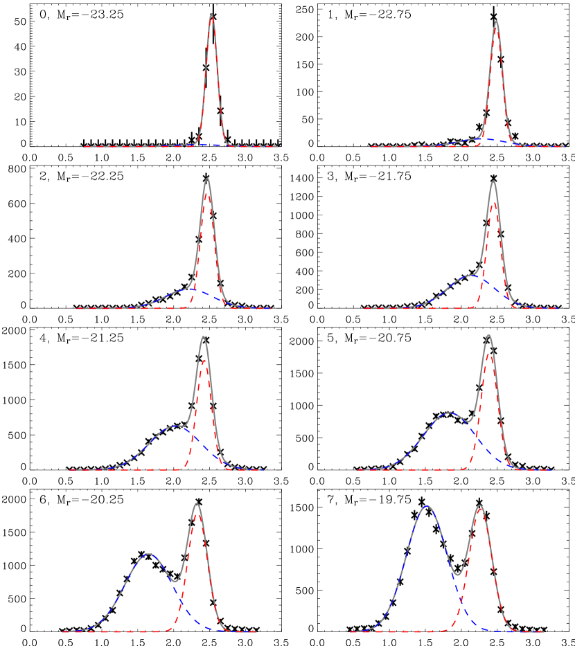
Figure 3.— Color functions for the galaxy distributions in absolute magnitude bins of width 0.5. Each plot shows galaxy number counts versus rest-frame $u-r$ color. The crosses with error bars represent the $V_{\rm survey}/V_{\rm max}$ corrected counts in 0.1 color bins. The solid lines represent double-Gaussian fits while the dashed lines represent the single Gaussians of the blue and red distributions.

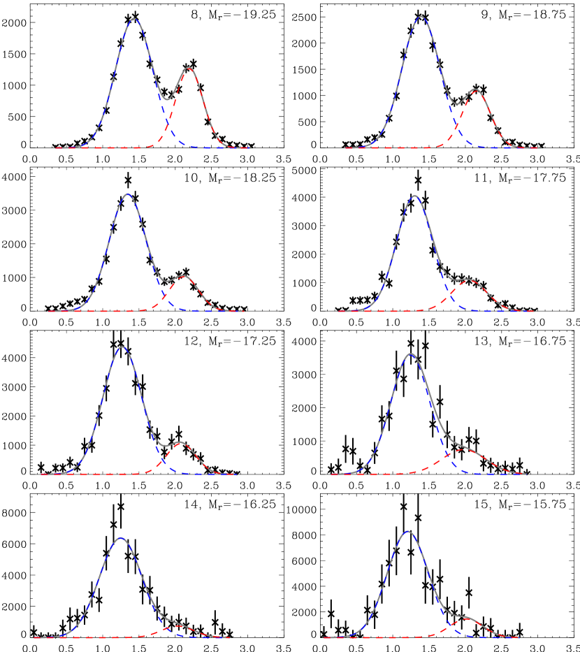
Figure 4.— Color functions for the galaxy distributions continued. See Figure 3 for details.

For two of the bins brighter than $-22$, there are significantly more galaxies on the blue side of the red distribution, justifying the continued use of the bimodal description. For the most luminous bin, there is no evidence of any blue distribution and we only have an upper limit on the density of blue-distribution galaxies here. For the three bins fainter than $-17$, there are more galaxies on the red side of the blue distribution than the blue side. Note that for the two brightest and two faintest bins, the mean and dispersion of the less-populous distribution are fixed by extrapolation from the whole population. The general trend is for the number-density ratio of the red to the blue distribution to increase with luminosity. In the following subsections, we describe: in 5.1, the CM relations for the two distributions; in 5.2, the luminosity functions; in 5.3, an optimum divider between the two types, and; in 5.4, a conversion to stellar mass.

5.1. Color-Magnitude Relations

To quantify these distributions further, we assume that the Gaussian parameters vary smoothly from one absolute magnitude bin to the next. The dispersion and mean of each distribution are fitted by straight line plus tanh functions (${\cal T}$ functions, five paras., Eqn. 9). These fits are shown in Figures 5 and 6. These ${\cal T}$ functions provide a far superior fit than a five-parameter (4th order) polynomial. In addition, they are more stable for extrapolation (a straight line at the outside limits) and they can be related more readily to a physical explanation (a general trend with luminosity plus a transition around a particular luminosity). Table 1 shows the fitted parameters with uncertainties. The parameters $p_{0}$ and $p_{1}$ represent the intercept and slope of the straight line while $q_{0}$, $q_{1}$ and $q_{2}$ represent the amplitude, midpoint and range of the transition.

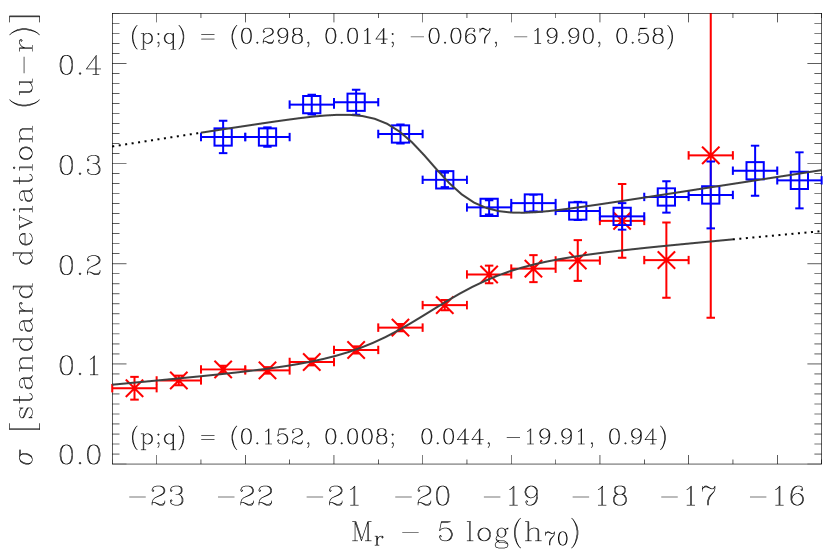
Figure 5.— Dispersion-magnitude relations: variation in the dispersion of the rest-frame $u-r$ colors for each galaxy distribution from the double-Gaussian fitting (crosses for $\sigma_{\rm r}(M_{r})$ and squares for $\sigma_{\rm b}(M_{r})$, with vertical error bars and horizontal bars representing the width of the magnitude bins). Note that the error bars can be smaller than the symbols. The solid lines represent straight line plus tanh function (Eqn. 9) fits to the data. The dotted lines represent an extrapolation where the parameters are fixed in the double-Gaussian fitting. The parameters for the fitted functions are shown in the plot. Note that the measured dispersion includes observational uncertainties.

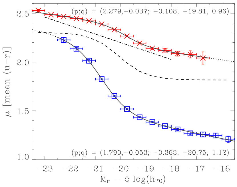
Figure 6.— Color-magnitude relations: variation in the mean of the rest-frame $u-r$ colors for each galaxy distribution (crosses for $\mu_{\rm r}(M_{r})$ and squares for $\mu_{\rm b}(M_{r})$, with vertical error bars). Note that the error bars can be smaller than the symbols. The dashed line represents an optimal divider between the two distributions (Sec. 5.3). The dash-and-dotted line shows the slope of the average $U-V$ CM relation of Bower et al. (1992b) for E+S0 galaxies in clusters ($-0.087$), offset from the red distribution for clarity. See Figure 5 for other details.

Table 1Color- and dispersion-magnitude relations: ${\cal T}$ function parameters^a

distribution	$p_{0}$	$p_{1}$	$q_{0}$	$q_{1}$	$q_{2}$	($q_{1}/$${\cal M}_{\odot}$)b
$\mu_{\rm r}$	$2.279\pm 0.006$	$-0.037\pm 0.006$	$-0.108\pm 0.017$	$-19.81\pm 0.07$	$0.96\pm 0.16$	1.8$\times 10^{10}$
$\sigma_{\rm r}$	$0.152\pm 0.006$	$0.008\pm 0.006$	$0.044\pm 0.018$	$-19.91\pm 0.18$	$0.94\pm 0.40$	2.0$\times 10^{10}$
$\mu_{\rm b}$	$1.790\pm 0.014$	$-0.053\pm 0.008$	$-0.363\pm 0.029$	$-20.75\pm 0.05$	$1.12\pm 0.10$	2.6$\times 10^{10}$
$\sigma_{\rm b}$	$0.298\pm 0.004$	$0.014\pm 0.007$	$-0.067\pm 0.014$	$-19.90\pm 0.07$	$0.58\pm 0.19$	0.9$\times 10^{10}$

^a The results of fitting a straight line plus a tanh function (Eqn. 9) to the variations, in the means ($\mu$) and dispersions ($\sigma$), of the red and blue distributions as a function of $M_{r}$ (Eqns. 7 and 8). The $p$ parameters represent the straight line while the $q$ parameters represent the tanh function. The fitted lines are shown in Figures 5 and 6. Note that the errors quoted do not include systematic uncertainties due to photometric calibration or $k$-corrections.
^b The transition midpoint approximately converted to stellar mass (see Section 5.4).

5.1.1 The red distribution

One of the most well-studied relations is the CM relation for luminous early-type galaxies (Visvanathan & Sandage, 1977; Sandage & Visvanathan, 1978a, b; Bower, Lucey, & Ellis, 1992a, b; Schweizer & Seitzer, 1992; Terlevich, Caldwell, & Bower, 2001; Bernardi et al., 2003). This corresponds approximately to the red distribution with $M_{r}\lesssim-20$ (Fig. 6). Our formal slope is about $-0.04$ ($p_{1}$ for $\mu_{\rm r}$) but we find that the slope gets steeper toward the transition midpoint at $-19.8$ ($q_{1}$).

Previous work found slopes of around $-0.1$ for the $u-V$ CM relation (Visvanathan & Sandage; Bower et al.; Terlevich et al.). The difference in slope between $u-r$ and $u-V$ relations is negligible (Visvanathan & Sandage) and therefore there is a non-trivial difference between our measured slope and previous work. The difference can largely be explained by the use of a $\cal T$-function fit rather than a straight-line fit because a straight-line fit to our data gives a slope of about $-0.08$.

Other factors that could contribute to a difference in slope are: field versus cluster environment; Gaussian color function fitting versus E+S0 morphological selection and; aperture effects (Scodeggio, 2001; Bernardi et al., 2003). However, the CM relation has been found to be similar between different environments (Sandage & Visvanathan; Terlevich et al.) and no significant difference has been found between E and S0 galaxies in the CM relation (Sandage & Visvanathan) and, therefore, all morphological types that are genuinely part of the red distribution may have a similar relation. An analysis of the difference between using SDSS model and other magnitude definitions for the CM relation is given by Bernardi et al. We note that SDSS model colors are weighted toward the center of a galaxy and therefore the relations presented here apply to that weighting (see Sec. 4.4.5.5 of Stoughton et al., 2002, for model fitting details).

For the color dispersion-magnitude relation (Fig. 5), we find only a modest slope at the bright end with low statistical significance ($p_{1}$ for $\sigma_{\rm r}$ is about 1 standard deviation from zero). This is consistent with the CM relation for $M_{r}\lesssim-21$ being due to a metallicity-luminosity correlation (Faber, 1973; Kodama & Arimoto, 1997) since dust reddening and SFH correlations could also introduce more scatter.

The dispersion-magnitude relation for the red distribution goes through a transition at the same magnitude, within the uncertainties, as the CM relation (Figs. 5 and 6; Table 1). This is consistent with the transition being due to an increasing contribution from recent star formation with decreasing galaxy luminosity (from $M_{r}$ of about $-21$ to $-19$; see also Ferreras & Silk 2000). The colors of younger stellar populations are more dependent on their ages than older populations (see e.g. fig. 1 of Bower et al., 1998), which implies more dispersion in a CM relation. In other words, if there has been on average more recent star formation in a class of galaxies, then their mean color becomes bluer and the color dispersion increases for any reasonable variation in their precise SFHs. However, we cannot rule out the transition also being caused by a metallicity-luminosity correlation as long as the metallicity dispersion increases with decreasing galaxy luminosity (Poggianti et al., 2001).

Note that our measurements of dispersion include observational uncertainties. At the bright-end, the measured dispersion is about 0.09, which is comparable to the observational uncertainties and is, therefore, consistent with an intrinsic dispersion of less than 0.05 (Visvanathan & Sandage, 1977; Bower et al., 1992b).

5.1.2 The blue distribution

Color-magnitude relations for late-type galaxies are also an established phenomenon (Visvanathan, 1981; Tully et al., 1982, 1998; Wyse, 1982; Peletier & de Grijs, 1998). Here, we precisely trace a CM relation over seven magnitudes and find that it is very well fit by a tanh function plus a straight line (Fig. 6).

For the low-luminosity blue-distribution galaxies ($M_{r}\gtrsim-19$), we find a shallow CM relation slope ($-0.05$) that is consistent with a metallicity-luminosity correlation for the following reasons. Studies of late-type galaxies yield a strong metallicity-luminosity relation down to low luminosities from their emission lines (Garnett, 2002; Tremonti et al., 2003) and from their stellar content (Bell & de Jong, 2000). In addition, the general slopes of the CM relations for the red and blue distributions, defined by the $p_{1}$ values (i.e. excluding the transition), are approximately the same (within $<2$ standard deviations). Modest correlations of luminosity with SFH and/or dust are also possible.

Over the luminosity range from $-19.5$ to $-22$ (increasing galaxy luminosity), we find a significant reddening of the blue sequence that is too steep to be explained entirely by a metallicity-luminosity correlation. This transition can be explained by a combination of an increase in dust content (Giovanelli et al., 1995; Tully et al., 1998) and a decrease in recent star formation relative to the total stellar mass of the galaxy (Peletier & de Grijs, 1998). These processes will have opposite effects on the dispersion. Increased dust content will increase dispersion, because of the range of reddening associated with different disk orientations, whereas decreased star formation will decrease dispersion because old stellar populations vary less in color (c.f. the luminous red distribution). Our interpretation of the dispersion-magnitude relation (Fig. 5) is then that the dust content increase dominates the transition from $-19.5$ to $-20.8$ ($\sigma_{\rm b}$ increases, $\mu_{\rm b}$ increases) and that the competing processes approximately cancel from $-20.8$ to $-22$ ($\sigma_{\rm b}$ decreases slightly, $\mu_{\rm b}$ increases). This explains why the tanh fit for $\sigma_{\rm b}$ does not coincide with that for $\mu_{\rm b}$ (Table 1). We take the genuine transition in the properties of the blue distribution to be that defined by the $\mu_{\rm b}$ fit.

5.2. Luminosity Functions

The results of fitting the amplitudes of the double-Gaussian functions are used to determine the luminosity functions (Eqn. 7) while the mean and dispersion of the CM relations are constrained to be ${\cal T}$ functions (Eqn. 9). The luminosity functions are shown in Figure 7 and Table 2. To fit to these luminosity functions, we increase the errors slightly in order to avoid being overly constrained by the high S/N bins, which could be dominated by systematic errors and in consideration of large-scale structure uncertainties. The results of fitting Schechter functions are shown in Figure 7 and Table 3. Overall, about 42% of the $r$-band luminosity density is in red-distribution galaxies. Not surprisingly, this is slightly larger than the 38% found to be in red-type galaxies by Hogg et al. (2002) because their definition of red-type was based on strict cuts in color, concentration and surface brightness.

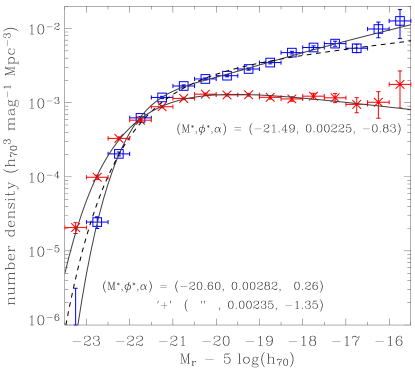
Figure 7.— Luminosity functions for each galaxy distribution (crosses for $\phi_{\rm r}(M_{r})$ and squares for $\phi_{\rm b}(M_{r})$, with error bars). The lines represent fits to the data. The dashed line for $\phi_{\rm b}$ and the solid line for $\phi_{\rm r}$ represent standard Schechter functions, while the solid line for $\phi_{\rm b}$ represents a double Schechter function with a single value for $M^{*}$. The standard single Schechter function does not provide a good fit to the blue distribution. The parameters for the single Schechter $\phi_{\rm r}$ and double Schechter $\phi_{\rm b}$ fits are shown in the plot.

Table 2Luminosity functions^a

$M_{r}-5\log h_{70}$	$\phi_{\rm r}\,h_{70}^{-3}$	$\phi_{\rm b}\,h_{70}^{-3}$
	(${\rm mag}^{-1}\,{\rm Mpc^{-3}}$)	(${\rm mag}^{-1}\,{\rm Mpc^{-3}}$)
$-23.25$	$(2.06\pm 0.35)\times 10^{-5}$	$(0.30\pm 2.83)\times 10^{-6}$
$-22.75$	$(0.99\pm 0.07)\times 10^{-4}$	$(2.45\pm 0.44)\times 10^{-5}$
$-22.25$	$(3.30\pm 0.15)\times 10^{-4}$	$(2.04\pm 0.12)\times 10^{-4}$
$-21.75$	$(5.81\pm 0.24)\times 10^{-4}$	$(6.24\pm 0.26)\times 10^{-4}$
$-21.25$	$(8.82\pm 0.33)\times 10^{-4}$	$(1.18\pm 0.04)\times 10^{-3}$
$-20.75$	$(1.14\pm 0.04)\times 10^{-3}$	$(1.68\pm 0.06)\times 10^{-3}$
$-20.25$	$(1.30\pm 0.05)\times 10^{-3}$	$(2.09\pm 0.07)\times 10^{-3}$
$-19.75$	$(1.27\pm 0.05)\times 10^{-3}$	$(2.31\pm 0.08)\times 10^{-3}$
$-19.25$	$(1.28\pm 0.06)\times 10^{-3}$	$(2.85\pm 0.10)\times 10^{-3}$
$-18.75$	$(1.18\pm 0.06)\times 10^{-3}$	$(3.48\pm 0.13)\times 10^{-3}$
$-18.25$	$(1.12\pm 0.08)\times 10^{-3}$	$(4.74\pm 0.20)\times 10^{-3}$
$-17.75$	$(1.23\pm 0.12)\times 10^{-3}$	$(5.56\pm 0.30)\times 10^{-3}$
$-17.25$	$(1.17\pm 0.16)\times 10^{-3}$	$(6.27\pm 0.49)\times 10^{-3}$
$-16.75$	$(0.95\pm 0.22)\times 10^{-3}$	$(5.43\pm 0.70)\times 10^{-3}$
$-16.25$	$(1.01\pm 0.40)\times 10^{-3}$	$(0.99\pm 0.24)\times 10^{-2}$
$-15.75$	$(1.77\pm 0.92)\times 10^{-3}$	$(1.27\pm 0.54)\times 10^{-2}$

^a Non-parametric luminosity functions for the red and blue distributions (see Eqn. 7). The errors include formal and systematic uncertainties. The latter include a constant 3% plus a fraction proportional to 1/$V_{\rm max}$ increasing to 40% for the lowest luminosity bin (to approximately account for large-scale structure effects). The functions are shown in Figure 7.

Table 3Schechter function fits to the luminosity functions^a

distribution	$M^{*}-5\log h_{70}$	$\phi^{*}\,h_{70}^{-3}$	$\alpha$	$\phi^{*}{}^{\prime}\,h_{70}^{-3}$	$\alpha^{\prime}$	$j+2.5\log h_{70}$b
		($10^{-3}\,{\rm Mpc^{-3}}$)		($10^{-3}\,{\rm Mpc^{-3}}$)		(${\rm Mpc^{-3}}$)
$\phi_{\rm r}$	$-21.49\pm 0.03$	$2.25\pm 0.08$	$-0.83\pm 0.02$	—	—	$-14.79$ (42%)
$\phi_{\rm b}$	$-20.60\pm 0.08$	$2.82\pm 0.32$	$+0.26\pm 0.21$	$2.35\pm 0.37$	$-1.35\pm 0.05$	$-15.13$ (58%)
$\phi_{\rm b}$	$-21.28\pm 0.03$	$2.89\pm 0.13$	$-1.18\pm 0.02$	—	—	$-15.08$

^a A single Schechter function was found to give a good fit to the red distribution ($\phi_{\rm r}$) but not to the blue distribution ($\phi_{\rm b}$). In the latter case, a significantly better fit was obtained by summing two Schechter functions (with a single value for $M^{*}$). Both the double- and single-Schechter function parameters are shown for $\phi_{\rm b}$.
^b The luminosity density in absolute magnitudes per Mpc³. The percentage in brackets is the fraction relative to the total $r$-band luminosity density.

Note that a single Schechter function was found to give a good fit to the red distribution but not to the blue distribution. In the latter case, there is a small but statistically significant slope change around $M_{r}\approx-20$. To account for this, we used a double-Schechter function but with the same value for $M^{*}$ (i.e. the sum of two power laws with one exponential cutoff, it was not necessary to allow two-different $M^{*}$ values to provide a good fit). The double-Schechter function provided a noticeably better fit to the faint end of the luminosity function with a steeper faint-end slope ($\alpha^{\prime}=-1.35$, the second power law dominates here) compared to the single Schechter fit ($\alpha=-1.18$). Note that this is purely a mechanism for obtaining a better fit to the luminosity function and it should not be interpreted as evidence for two blue populations.

The red distribution has a significantly shallower faint-end slope ($\alpha=-0.83$) than the blue distribution. Related results have been found by dividing galaxies into classes from early to late spectral types: Madgwick et al. (2002) found faint-end slopes from $-0.5$ to $-1.5$ based on emission and absorption line strengths in optical spectra, and; Blanton et al. (2001) found a steepening of the slope from red to blue galaxies based on cuts in $g-r$ color (their fig. 14). However, the equivalent steepening of the faint-end slope toward late types based on morphological classification appears less significant (Nakamura et al., 2003). This is not inconsistent with our result since the red and blue distributions at the faint and bright ends need not have the same mix of morphological types. In other words, the processes that result in the red (or the blue) distribution also produce a range of morphological types that need not be the same at low and high luminosities.

5.3. Dividing the Distribution

One of the ways to divide a galaxy sample is by absolute magnitude to compare, for example, galaxy clustering relations (Zehavi et al., 2002). Figure 8 shows the ratio between the luminosity functions as a function of absolute magnitude. The ratio of the red distribution to the total galaxy population gradually increases from low luminosities to $M_{r}\approx-22$. For galaxies more luminous than this, the fraction of the population derived from the red distribution increases more rapidly. This agrees with the standard result that the most luminous galaxies are almost entirely early types (e.g. Blanton et al., 2003c).

Figure 8.— Fraction of galaxies that are part of the red distribution as a function of absolute magnitude: $\phi_{\rm r}(M_{r})$ / [$\phi_{\rm r}(M_{r})+\phi_{\rm b}(M_{r})]$. The diamonds with error bars represent the ratios determined from the non-parametric luminosity functions (Table 2) while the dashed line represents the ratios determined from the Schechter function fits (Table 3).

We can also look at divisions in color and absolute magnitude space. Figure 9 shows the bivariate distribution separated into the two types based on the analysis in this paper. In general, it is possible to define regions of the space that are almost entirely derived from one distribution except, notably, for a region around $M_{r}\sim-21.5$ and $C_{ur}\sim 2.5$. Here, dusty and/or bulge-dominated spirals ‘overlap’ in this space with old stellar-population ellipticals. A related result was obtained by Hogg et al. (2003), studying “the overdensities of galaxy environments as a function of luminosity and color”, where luminous red and faint red galaxies were found, on average, in more overdense regions than $M^{*}$ red galaxies (see their fig. 2). Our analysis can explain this result because of the blue distribution interlopers, formed by a different set of processes, with similar colors to the $M^{*}$ red distribution galaxies.

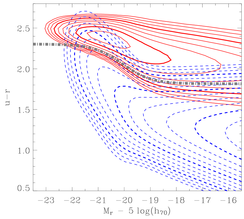
Figure 9.— Empirical red and blue bivariate distributions ($\Phi_{\rm r}$ and $\Phi_{\rm b}$) using the parameterization of Section 4.1 with values from Tables 1 and 3. The solid contours represent the red distribution, while the dashed contours represent the blue distribution. The contour levels are on a logarithmic scale, starting at an arbitrary level and doubling every two contours. The thick dash-and-dotted line represents an optimal divider (Sec. 5.3). Note that the measured dispersion includes observational uncertainties, which implies that the luminous red ‘ridge’ is, in reality, significantly narrower.

Modeling a distribution with two sequences in this way naturally leads to a physical model with two kinds of galaxies with different processes associated with them. Therefore, it would be appropriate to study the properties of each distribution separately. However, this is not precisely possible because of the dispersions and overlaps associated with each distribution. Instead, we can make an optimal divider by defining figure of merits based on the double-Gaussian description. Following Strateva et al. (2001), for any cut on color, we can estimate the ‘completeness’ (${\cal C}$) and ‘reliability’ (${\cal R}$) of a sample. For example, if we use $C_{ur}>C^{\prime}_{ur}$ to select the red distribution then: ${\cal C}_{\rm r}$ is the fraction of galaxies from the red distribution that are selected, and; ${\cal R}_{\rm r}$ is the fraction of galaxies selected that derive from the red distribution (i.e. $1-{\cal R}_{\rm r}$ is the contamination from the blue distribution).

There are many ways to define an optimum divider in color as a function of absolute magnitude based on different weightings of completeness and reliability. They can be determined using the parameterized description of the data described in this paper. Here, we define an optimum divider that best selects red distribution galaxies redder than the color cut and vice versa simultaneously, with a figure of merit defined by ${\cal C}_{\rm r}{\cal R}_{\rm r}{\cal C}_{\rm b}{\cal R}_{\rm b}$. This optimal divider (parameterized by a tanh function) is given by

$$C^{\prime}_{ur}(M_{r})=2.06-0.244\tanh\left[\frac{M_{r}+20.07}{1.09}\right]$$ (11)

and is shown in Figures 6 and 9. The optimal color division varies from about 2.3 at the bright end to 1.8 at the faint end of the galaxy distribution. For galaxies fainter than $M_{r}$ of $-21$, we obtain ${\cal C}_{\rm r}>0.8$, ${\cal R}_{\rm r}>0.8$, ${\cal C}_{\rm b}>0.85$ and ${\cal R}_{\rm b}>0.95$ at all magnitudes, but for more luminous galaxies, both ${\cal C}_{\rm b}$ and ${\cal R}_{\rm r}$ drop below 0.8 due to the increased overlap of the blue distribution with the red distribution (${\cal R}_{\rm r}$ rises again for the most luminous two or three bins because of the thinning out of the blue distribution).

5.4. Conversion to Stellar Mass

In terms of relating variations in galaxy properties to models of galaxy formation and evolution, it is more appropriate to consider stellar mass than luminosity because stellar mass is more closely related to baryon content. Stellar mass-to-light ratios (${\cal M}/L$) can vary by up to a factor of about ten for the $r$-band luminosity. However, ${\cal M}/L$ can be estimated by fitting population-synthesis models to colors or spectroscopic indices (Brinchmann & Ellis, 2000; Bell et al., 2003a; Kauffmann et al., 2003a). In order to convert our results to stellar-mass relations, we use an approximate color-${\cal M}/L$ conversion given by

$$\log({\cal M}/{L_{r}})\>=\>a\,+\,b\,C_{ur}$$ (12)

where $(a,b)=(-0.55,0.45)$ and; ${\cal M}$ and $L_{r}$ are the mass and specific luminosity in solar units. This is a useful approximation because there is a significant correlation between $u-r$ and ${\cal M}/L$.

The coefficients in Equation 12 were derived from an average of analyses based on the stellar masses of Bell et al. (2003a) and Kauffmann et al. (2003a), for which we obtained $(a,b)\approx(-0.3,0.35)$ and $(-0.8,0.55)$, respectively, by fitting log (stellar mass) as a function of $(u-r)_{\rm model}$ for low redshift galaxies ($z<0.08$). The assumed stellar IMFs were similar between the two analyses, and therefore the differences arise principally from the methodologies (see Bell et al. and Kauffmann et al. for details). This gives us some estimate of the systematic uncertainties involved with this type of modeling. For the stellar-mass ranges quoted in this section (below), we use the $a,b$ coefficients given above and include uncertainties from our fitting. Note that we do not include uncertainties in the stellar IMF (or, e.g. evolutionary tracks), which could amount to $\sim$30% uncertainty in the absolute values of the stellar masses, and the conversion to total mass is considerably more uncertain due to the dominance of dark matter in most galaxies.

For simplicity, we apply the ${\cal M}/L$ adjustment (Eqn. 12) to the relations and luminosity functions using the $\mu_{\rm r}$ and $\mu_{\rm b}$ values as a function of absolute magnitude (Table 1). This is a reasonable adjustment for the average galaxies in each distribution. Figure 10 shows the luminosity functions adjusted for stellar mass-to-light ratios, in effect, galaxy stellar mass functions (GSMFs). The parameters for the Schechter fits are shown in the plot. The red distribution is shifted to higher masses with respect to the blue distribution. The stellar mass density per magnitude is dominated by the red distribution for galaxy stellar masses greater than about (2–5) $\times 10^{10}$ ${\cal M}_{\odot}$. Overall, about 54%–60% of the stellar mass density is in red-distribution galaxies (depending on the coefficients of the approximate conversion to stellar mass).

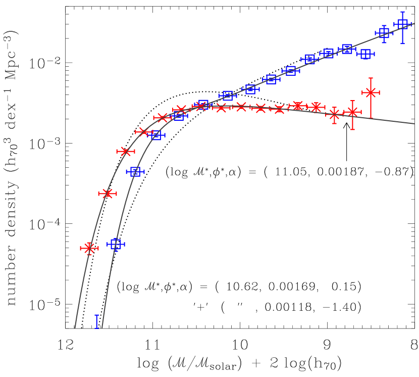
Figure 10.— Galaxy stellar mass functions, for each distribution, derived from luminosity functions adjusted to account for variations in the stellar mass-to-light ratio as a function of color (Eqn. 12). Note that, as well as the $x$-axis being adjusted, the number density is adjusted to account for the stretching of the magnitude bins and the conversion to base-ten logarithms. The solid lines represent the Schechter functions fits to our data while dotted lines represent the color-selected early- and late-type GSMF fits of Bell et al. (2003a). See Figure 7 for other details.

In Figure 10, we also plot the color-selected early- and late-type GSMFs of Bell et al. (2003a). Notably, the early types have a significantly higher number density per magnitude relative to the late types around ${\cal M}^{*}$ whereas the GSMFs from the double-Gaussian fitting have similar number densities here. This reflects the fact that our analysis quantifies an overlap in color space (Fig. 9), and thus enhances the ‘late type’ number density compared to a standard color selection, even if using a slope in $g-r$ versus $M_{r}$ (as per Bell et al.).

The transitions in galaxy properties occur around (1.5–2.2) $\times 10^{10}$ ${\cal M}_{\odot}$ for the red distribution ($q_{1}$ for $\mu_{\rm r}$ and $\sigma_{\rm r}$) and around (2–3) $\times 10^{10}$ ${\cal M}_{\odot}$ for the blue distribution ($q_{1}$ for $\mu_{\rm b}$), based on converting the CM relations (see Table 1). Despite our simplistic treatment of ${\cal M}/L$ conversions (which do not differentiate between dust attenuation and SFH effects), our transition masses are close to the transition in galaxy properties noted by Kauffmann et al. (2003b) that occurred around $3\times 10^{10}$ ${\cal M}_{\odot}$. Here, we have resolved this transition into three different effects, a change in dominance from one distribution to the other, a change in the properties of the red distribution and a change in the blue distribution.

6. Conclusions

We have devised a new method of analysing color-magnitude relations based on considering double-Gaussian distributions in color (Figs. 3 and 4) rather than strict cuts on morphological or other properties. From this, we obtain CM and dispersion-magnitude relations for two dominant red and blue distributions, which can in general be associated with classical definitions of early- and late-type galaxies. These relations are evident across seven magnitudes (Figs. 5 and 6) but are not well fit by a straight line. Instead, we find that a straight line plus a tanh function provides good fits (Eqn. 9, Table 1).

For both the red and blue distributions, we can associate the general trend (the straight line part of the combined function) with a universal metallicity-luminosity correlation. The tanh function can be associated with a transition in other properties of the galaxy population, which could include star-formation history and dust attenuation (in the case of late types). Note we have not proved the above physical explanations but have obtained them from previous results and analyses in the literature (e.g. Zaritsky et al., 1994; Kodama & Arimoto, 1997; Peletier & de Grijs, 1998; Tully et al., 1998; Garnett, 2002; Kauffmann et al., 2003b). Further work is required, e.g. population synthesis fitting to SDSS spectra, to bolster and quantify the physical explanations for these relations.

After converting to stellar mass, we find that the midpoints of the transitions parameterized by the tanh functions are around $2\times 10^{10}$ ${\cal M}_{\odot}$ (Table 1). In addition, we find that the number density per magnitude of the red distribution overtakes the blue distribution at about $3\times 10^{10}$ ${\cal M}_{\odot}$ (Fig. 10). These changes in properties of the galaxy population are in good agreement with the transition found by Kauffmann et al. (2003b) at $3\times 10^{10}$ ${\cal M}_{\odot}$ using spectroscopic measurements.

In order to study the physical properties of each distribution separately, it is necessary to divide them. To do this, we defined an optimum divider based on minimizing the overlap between the two Gaussian descriptions (Eqn. 11, Fig. 9). We note that this works well for galaxies fainter than $M_{r}\sim-21$. For galaxies more luminous than this, morphological indicators that also show a bimodality can work better at dividing the population into two types. Thus, a weighted combination of various measurements (from photometry, spectroscopy and morphology) could provide a better division by type, with the weights varying with absolute magnitude.

The luminosity functions of the two distributions are significantly different from each other (Figs. 7 and 8, Tables 2 and 3). The red distribution luminosity function has a shallower faint-end slope and a more luminous characteristic magnitude. The difference between the two distributions can be explained in terms of a merger scenario where the red distribution derives from more major mergers. To show this, we first approximately converted the luminosity functions to galaxy stellar mass functions (Fig. 10) and fitted a simple numerical model to the data (Fig. 11). Some discussion of mergers and a description of the model is given in the Appendix. This is consistent with hierarchical clustering theories.

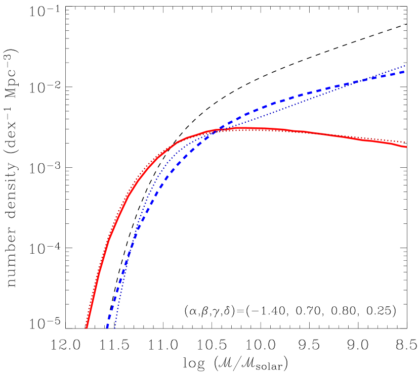
Figure 11.— Simulated galaxy stellar mass functions, for each distribution, from a simple merger model (solid line and thick dashed line for the red and blue distributions, respectively). See the Appendix for details of the model. The merger scenario produces a shallower faint-end slope and a more massive characteristic mass for the red distribution compared to the blue distribution. The dotted lines represent the Schechter function fits to our data (Fig. 10) while the thin dashed line represents the initial function in the model. The parameters for the model are shown in the plot and relate to: initial faint-end slope ($\alpha$); mass exponent for weighting in the merger model ($\beta$); probability of a faint galaxy merging with a more massive galaxy ($\gamma$), and; fractional increase in mass from merging used to determine which galaxies are part of the red distribution ($\delta$).

Finally, we note that further work could proceed in a number of directions including: (i) defining an optimum division between the two distributions by combining various observed quantities; (ii) analysing the spectra of each distribution; (iii) studying the distributions of the morphological properties; (iv) comparing the CM relations between different galaxy environments, and; (v) simulating galaxy mergers and hierarchical clustering to test the cause of the bimodality. Here, we propose that the double-Gaussian fitting technique represents a model-independent way of defining a ‘post-major-merger’ sequence, in that the uncertainties due to blue-distribution interlopers are quantified, without using a semi-arbitrary cut in morphology or spectral type.

Appendix A A Simple Merger Model

Early-type galaxies tend to have more spherical geometries, more virialized motions of stars, less dust as well as redder colors. N-body simulations suggest that the geometries and the motions of stars, similar to those observed in ellipticals, can be produced by galaxy mergers (Barnes, 1988; Barnes & Hernquist, 1992). In addition, if the merger causes the gas and dust to be expelled and/or used up in a burst of star formation (Joseph & Wright, 1985) then the galaxy’s star-formation rate will be lower (at some later time) than star-forming late-type galaxies. This in turn will mean redder colors for galaxies produced by mergers as long as any induced star burst does not dominate the stellar population or the merger occurred at high redshift, i.e. as long as most of the stars formed at high redshift (Baugh, Cole, & Frenk, 1996; Kauffmann, 1996). Kauffmann & Charlot (1998) have shown that a hierarchical merger model can reproduce the CM relation of cluster ellipticals.

Given these lines of argument, it is reasonable to suppose that mergers are the cause of the bimodality, with the red distribution deriving from major merger processes and the blue distribution deriving from more quiescent accretion (with only minor mergers at most). To test this, we devised an illustrative non-dynamical merger model to see if the basic shapes of the GSMFs (Fig. 10) with respect to each other could be explained. The procedure for this model is described below.

1. A population of galaxies is created with an initial baryonic-mass function described by a Schechter function with a faint-end slope $\alpha$ (for simplicity, we assume that all the baryons will be used to form stars and thus can be related to the GSMFs observed today). The population is defined from about $10^{-3}\,{\cal M}^{*}$ to $10\,{\cal M}^{*}$. The characteristic mass and number density, ${\cal M}^{*}$ and $\phi^{*}$, are adjusted to best match the data after the simulation.

2. These galaxies are numbered from 1 to $N_{\rm gals}$ in order of increasing mass.

3. For each galaxy $i$, it is determined whether it will merge with a more massive galaxy based on a probability equal to

   $$p_{i}=\left(\frac{\sum_{j=i+1}^{N_{\rm gals}}{\cal M}_{j}^{\beta}}{\sum_{j=1}^{N_{\rm gals}}{\cal M}_{j}^{\beta}}\right)\gamma$$ (A1)

   where ${\cal M}_{j}$ is the initial mass of the $j$-th galaxy. In other words, the probability is the sum of the more massive galaxies weighted by mass with an exponent $\beta$, divided by the total mass in the population, multiplied by $\gamma$. The probability of the lowest mass galaxy merging with another galaxy is approximately $\gamma$.

4. For each merged galaxy $i$, the mass is added to another galaxy at random but with a weighting proportional to ${\cal M}_{j}^{\beta}$ for $j>i$ (and 0 for $j<i$).

5. For each remaining galaxy, the fractional increase of its mass relative to its initial mass is determined. Galaxies with fractional increases greater than $\delta$ are determined to be in the red distribution (similar to the $f_{\rm ellip}$ parameter of Kauffmann, White, & Guiderdoni, 1993).

6. The model GSMFs for the red and blue distributions are determined and ${\cal M}^{*}$ and $\phi^{*}$ are adjusted to best fit the data, over the ranges $8.6<\log{\cal M}^{*}<11.8$ for the red and $8.4<\log{\cal M}^{*}<11.6$ for the blue distribution.

The additional physical assumptions behind this scenario are: that galaxies form from quiescent accretion with a distribution in masses defined by a Schechter function, and; the probability of merging with a more massive galaxy is related to the number density and masses of all these galaxies. The model is simple in the sense that it is non-dynamical, the timing of accretion and merging is not accounted for, and the parameter $\beta$ hides the complex physics associated with forces on dark-matter haloes and their baryon contents. Note also that we do not model the CM relations, only the GSMFs.

Figure 11 shows a best-fit example of the simulated GSMFs from this simple merger model. It reproduces the shape of the red-distribution GSMF with high accuracy and the approximate faint-end slope of the blue distribution (though the shape is slightly different). Thus, the different luminosity functions (or GSMFs) can be explained if the red distribution is derived from galaxies where more than a certain fraction of their mass has come from mergers rather than ‘normal’ quiescent accretion. In other words, the red distribution is a post-major-merger sequence where ‘major’ is determined by the ratios of the masses of the merging galaxies. This sequence could also include galaxies derived from the sum of many minor mergers, which could evolve a galaxy from a spiral to an S0 (Walker, Mihos, & Hernquist, 1996).

References

- Abazajian et al. (2003) Abazajian, K. et al. 2003, AJ, in press (astro-ph/0305492)
- Baldry & Glazebrook (2003) Baldry, I. K. & Glazebrook, K. 2003, ApJ, 593, 258
- Barnes (1988) Barnes, J. E. 1988, ApJ, 331, 699
- Barnes & Hernquist (1992) Barnes, J. E. & Hernquist, L. 1992, ARA&A, 30, 705
- Baugh et al. (1996) Baugh, C. M., Cole, S., & Frenk, C. S. 1996, MNRAS, 283, 1361
- Baum (1959) Baum, W. A. 1959, PASP, 71, 106
- Bell & de Jong (2000) Bell, E. F. & de Jong, R. S. 2000, MNRAS, 312, 497
- Bell & de Jong (2001) —. 2001, ApJ, 550, 212
- Bell et al. (2003a) Bell, E. F., McIntosh, D. H., Katz, N., & Weinberg, M. D. 2003a, ApJS, in press (astro-ph/0302543)
- Bell et al. (2003b) Bell, E. F., Wolf, C., Meisenheimer, K., Rix, H., Borch, A., Dye, S., Kleinheinrich, M., & McIntosh, D. H. 2003b, ApJ, submitted (astro-ph/0303394)
- Bernardi et al. (2003) Bernardi, M. et al. 2003, AJ, 125, 1882
- Blanton et al. (2003a) Blanton, M. R., Lin, H., Lupton, R. H., Maley, F. M., Young, N., Zehavi, I., & Loveday, J. 2003a, AJ, 125, 2276
- Blanton et al. (2001) Blanton, M. R. et al. 2001, AJ, 121, 2358
- Blanton et al. (2003b) —. 2003b, AJ, 125, 2348
- Blanton et al. (2003c) —. 2003c, ApJ, 594, 186
- Bower et al. (1998) Bower, R. G., Kodama, T., & Terlevich, A. 1998, MNRAS, 299, 1193
- Bower et al. (1992a) Bower, R. G., Lucey, J. R., & Ellis, R. S. 1992a, MNRAS, 254, 589
- Bower et al. (1992b) —. 1992b, MNRAS, 254, 601
- Brinchmann & Ellis (2000) Brinchmann, J. & Ellis, R. S. 2000, ApJ, 536, L77
- Budavari et al. (2003) Budavari, T. et al. 2003, ApJ, in press (astro-ph/0305603)
- Chester & Roberts (1964) Chester, C. & Roberts, M. S. 1964, AJ, 69, 635
- Faber (1973) Faber, S. M. 1973, ApJ, 179, 731
- Ferreras & Silk (2000) Ferreras, I. & Silk, J. 2000, ApJ, 541, L37
- Fukugita et al. (1996) Fukugita, M., Ichikawa, T., Gunn, J. E., Doi, M., Shimasaku, K., & Schneider, D. P. 1996, AJ, 111, 1748
- Garnett (2002) Garnett, D. R. 2002, ApJ, 581, 1019
- Giovanelli et al. (1995) Giovanelli, R., Haynes, M. P., Salzer, J. J., Wegner, G., da Costa, L. N., & Freudling, W. 1995, AJ, 110, 1059
- Griersmith (1980) Griersmith, D. 1980, AJ, 85, 1295
- Gunn et al. (1998) Gunn, J. E. et al. 1998, AJ, 116, 3040
- Hogg et al. (2001) Hogg, D. W., Finkbeiner, D. P., Schlegel, D. J., & Gunn, J. E. 2001, AJ, 122, 2129
- Hogg et al. (2002) Hogg, D. W. et al. 2002, AJ, 124, 646
- Hogg et al. (2003) —. 2003, ApJ, 585, L5
- Holmberg (1958) Holmberg, E. 1958, Meddelanden Lunds Astron. Obser. Ser. II, 136, 1
- Joseph & Wright (1985) Joseph, R. D. & Wright, G. S. 1985, MNRAS, 214, 87
- Kauffmann (1996) Kauffmann, G. 1996, MNRAS, 281, 487
- Kauffmann & Charlot (1998) Kauffmann, G. & Charlot, S. 1998, MNRAS, 294, 705
- Kauffmann et al. (1993) Kauffmann, G., White, S. D. M., & Guiderdoni, B. 1993, MNRAS, 264, 201
- Kauffmann et al. (2003a) Kauffmann, G. et al. 2003a, MNRAS, 341, 33
- Kauffmann et al. (2003b) —. 2003b, MNRAS, 341, 54
- Kodama & Arimoto (1997) Kodama, T. & Arimoto, N. 1997, A&A, 320, 41
- Kroupa (2001) Kroupa, P. 2001, MNRAS, 322, 231
- Kroupa (2002) —. 2002, Science, 295, 82
- Larson (1974) Larson, R. B. 1974, MNRAS, 169, 229
- Lupton et al. (2001) Lupton, R. H., Gunn, J. E., Ivezić, Z., Knapp, G. R., Kent, S., & Yasuda, N. 2001, in ASP Conf. Ser. 238, Astronomical Data Analysis Software and Systems X, ed. F. R. Harnden, F. A. Primini, & H. E. Payne (San Francisco: ASP), 269
- Madgwick et al. (2002) Madgwick, D. S. et al. 2002, MNRAS, 333, 133
- Nakamura et al. (2003) Nakamura, O., Fukugita, M., Yasuda, N., Loveday, J., Brinkmann, J., Schneider, D. P., Shimasaku, K., & SubbaRao, M. 2003, AJ, 125, 1682
- Peletier & de Grijs (1998) Peletier, R. F. & de Grijs, R. 1998, MNRAS, 300, L3
- Petrosian (1976) Petrosian, V. 1976, ApJ, 209, L1
- Pier et al. (2003) Pier, J. R., Munn, J. A., Hindsley, R. B., Hennessy, G. S., Kent, S. M., Lupton, R. H., & Ivezić, Ž. 2003, AJ, 125, 1559
- Poggianti et al. (2001) Poggianti, B. M. et al. 2001, ApJ, 562, 689
- Roberts & Haynes (1994) Roberts, M. S. & Haynes, M. P. 1994, ARA&A, 32, 115
- Salpeter (1955) Salpeter, E. E. 1955, ApJ, 121, 161
- Sandage & Visvanathan (1978a) Sandage, A. & Visvanathan, N. 1978a, ApJ, 223, 707
- Sandage & Visvanathan (1978b) —. 1978b, ApJ, 225, 742
- Schechter (1976) Schechter, P. 1976, ApJ, 203, 297
- Schlegel et al. (1998) Schlegel, D. J., Finkbeiner, D. P., & Davis, M. 1998, ApJ, 500, 525
- Schweizer & Seitzer (1992) Schweizer, F. & Seitzer, P. 1992, AJ, 104, 1039
- Scodeggio (2001) Scodeggio, M. 2001, AJ, 121, 2413
- Shimasaku et al. (2001) Shimasaku, K. et al. 2001, AJ, 122, 1238
- Smith et al. (2002) Smith, J. A. et al. 2002, AJ, 123, 2121
- Stoughton et al. (2002) Stoughton, C. et al. 2002, AJ, 123, 485
- Strateva et al. (2001) Strateva, I. et al. 2001, AJ, 122, 1861
- Strauss et al. (2002) Strauss, M. A. et al. 2002, AJ, 124, 1810
- Terlevich et al. (2001) Terlevich, A. I., Caldwell, N., & Bower, R. G. 2001, MNRAS, 326, 1547
- Tremonti et al. (2003) Tremonti, C. A. et al. 2003, in preparation
- Tully et al. (1982) Tully, R. B., Mould, J. R., & Aaronson, M. 1982, ApJ, 257, 527
- Tully et al. (1998) Tully, R. B., Pierce, M. J., Huang, J., Saunders, W., Verheijen, M. A. W., & Witchalls, P. L. 1998, AJ, 115, 2264
- Uomoto et al. (1999) Uomoto, A. et al. 1999, Bull. American Astron. Soc., 31, 1501
- Visvanathan (1981) Visvanathan, N. 1981, A&A, 100, L20
- Visvanathan & Griersmith (1977) Visvanathan, N. & Griersmith, D. 1977, A&A, 59, 317
- Visvanathan & Sandage (1977) Visvanathan, N. & Sandage, A. 1977, ApJ, 216, 214
- Walker et al. (1996) Walker, I. R., Mihos, J. C., & Hernquist, L. 1996, ApJ, 460, 121
- Worthey et al. (1995) Worthey, G., Trager, S. C., & Faber, S. M. 1995, in ASP Conf. Ser. 86, Fresh Views of Elliptical Galaxies, ed. A. Buzzoni, A. Renzini, & A. Serrano (San Francisco: ASP), 203
- Wyse (1982) Wyse, R. F. G. 1982, MNRAS, 199, 1P
- Wyse (1997) —. 1997, ApJ, 490, L69
- York et al. (2000) York, D. G. et al. 2000, AJ, 120, 1579
- Zaritsky et al. (1994) Zaritsky, D., Kennicutt, R. C., & Huchra, J. P. 1994, ApJ, 420, 87
- Zehavi et al. (2002) Zehavi, I. et al. 2002, ApJ, 571, 172