Weak lensing shear and aperture-mass from linear to non-linear scales

Abstract

In this paper we describe the predictions for the smoothed weak lensing shear and aperture-mass of two simple analytical models of the density field: the minimal tree-model and the stellar model. Both models give identical results for the statistics of the 3-d density contrast smoothed over spherical cells and only differ by the detailed angular dependence of the many-body density correlations. We have shown in previous work that they also yield almost identical results for the pdf of the smoothed convergence, $\kappa_{s}$. We find that both models give rather close results for both the shear and the positive tail of the aperture-mass. However, we note that at small angular scales ($\theta_{s}\la 2^{\prime}$) the tail of the pdf ${\cal P}(M_{\rm ap})$ for negative $M_{\rm ap}$ shows a strong variation between the two models and the stellar model actually breaks down for $\theta_{s}\la 0.4^{\prime}$ and $M_{\rm ap}<0$. This shows that the statistics of the aperture-mass provides a very precise probe of the detailed structure of the density field, as it is sensitive to both the amplitude and the detailed angular behaviour of the many-body correlations. On the other hand, the minimal tree-model shows good agreement with numerical simulations over all scales and redshifts of interest, while both models provide a good description of the pdf ${\cal P}(\gamma_{is})$ of the smoothed shear components. Therefore, the shear and the aperture-mass provide robust and complimentary tools to measure the cosmological parameters as well as the detailed statistical properties of the density field.

1 Introduction

Magnification and shearing in the images of high-redshift galaxies arise naturally due to gravitational lensing effects. These effects derive from the fluctuations in the gravitational potential related to the underlying density field. Statistical analysis of such observed weak lensing data is therefore very effective in probing the underlying density, which is assumed to be dominated by the dark matter content. Observational surveys (see, e.g., Bacon, Refregier & Ellis, 2000, Hoekstra et al., 2002, Van Waerbeke et al., 2000, and Van Waerbeke et al., 2002) have consequently been particularly fruitful in this regard and have enabled estimates for the cosmological parameters to be made.

To model weak gravitational lensing, cosmological $N$-body simulations have been widely used in which the particle and mass distributions have been set to reflect those expected in the real universe. The first numerical studies for gravitational lensing employing $N$-body simulations used ray-tracing methods (see, e.g., Schneider & Weiss, 1988, Jarosszn’ski et al., 1990, Wambsganns, Cen & Ostriker, 1998, Van Waerbeke, Bernardeau & Mellier, 1999, and Jain, Seljak & White, 2000) to follow the deflections of light from sources at high redshift in the simulations. More recently, Couchman, Barber & Thomas (1999) developed an algorithm to compute the full 3-dimensional shear matrices at locations along lines of sight throughout simulation volumes. Barber (2002) extended the method to combine the shear matrices in the appropriate fashion along the lines of sight to produce final Jacobian matrices from which the weak lensing statistics could be directly derived.

On large angular scales, analytical computations for weak lensing statistics can readily be made, as this is the regime where perturbative calculations apply (e.g., Villumsen, 1996, Stebbins, 1996, Bernardeau et al., 1997, Jain & Seljak, 1997, Kaiser, 1998, Van Waerbeke, Bernardeau & Mellier, 1999, and Schneider et al., 1998). However, on small angular scales, especially relevant to observational surveys with small sky coverage, perturbative calculations are no longer valid and models to represent the gravitational clustering in the non-linear regime have been devised.

To describe the non-linear evolution of the matter power spectrum, Hamilton et al. (1991) proposed a technique based on a non-local transformation. Their method was extended by Peacock & Dodds (1996) and included the conservation of mass and the rescaling of physical lengths in the different regimes, following the “stable-clustering” Ansatz of Peebles (1980). More recently, Peacock & Smith (2000) and Seljak (2000) developed the “Halo Model” for the non-linear evolution. This model is able to reproduce the matter power spectrum of $N$-body simulations over a wide range of scales and relates the linear and non-linear power at the same scale through fitting formulæ. In a more recent development, Smith et al. (2002) have presented a new set of fitting functions based on the Halo Model and calibrated to a set of $N$-body simulations.

Barber & Taylor (2003) have now shown excellent agreement between the power spectrum in the lensing convergence obtained from numerical simulations in which they calculated the full 3-dimensional shear matrices along lines of sight and the predictions from the Halo model fitting functions of Smith et al. (2002).

An alternative approach used to describe the probability distribution function of the density field, from which the associated weak lensing statistics can be obtained, has been based directly on the many-body correlations. The most common model of this kind expresses the $p-$point correlations as a sum of $p-1$ products over the two-point correlations linking all $p$ points. This yields the class of “Hierarchical models,” which are specified by the weights given to any such topology associated with the $p-1$ products (e.g., Fry 1984, Schaeffer 1984, Bernardeau & Schaeffer 1992, and Szapudi & Szalay 1993, 1997, Munshi et al. 1999a, Munshi, Melott, Coles 1999d). Once these weights have been assigned it is possible to resum all many-body correlations and to compute the pdf of the density field, or of any quantity which is linearly dependent on the matter density. This is most easily done for “minimal tree-models”, where the weight associated to a given tree-topology is set by its vertices (e.g., Bernardeau & Schaeffer 1992, Munshi, Coles & Melott 1999b, Munshi, Coles & Melott 1999d), or for “stellar models”, which only contain stellar diagrams (Valageas, Barber & Munshi, 2003).

Using such an approach, coupled to the Hamilton et al. (1991) prescription for the two-point correlation, Valageas (2000a, b) and Munshi & Jain (2000 and 2001), Munshi & Coles (2000,2002) were able to compute the pdf of the weak-lensing convergence whilst the associated bias was considered by Munshi (2000) and the cumulant correlators associated with such distributions were evaluated by Munshi & Jain (2000). Munshi & Wang (2003) further extended these studies to cosmological scenarios including dark energy. These methods can also handle more intricate quantities like the aperture-mass or the shear which involve compensated filters and require a detailed model for the many-body correlations. Thus, using a minimal tree-model for the non-linear regime, Bernardeau and Valageas (2000) were able to predict the pdf of the aperture-mass and to obtain a good agreement with numerical simulations (they also showed that similar techniques could be applied to the quasi-linear regime where the calculations can actually be made rigorous). On the other hand, adopting a stellar model for the many-body correlations, Valageas, Barber & Munshi (2004) obtained excellent agreement for the shear pdf when compared with the results of $N$-body simulations. In a more recent paper, Barber, Munshi & Valageas (2004) described the results for the pdf of the convergence based on hierarchical models and again showed excellent agreement with the results from $N$-body simulations.

In this paper, we employ the minimal-tree model and the stellar model for the density field to predict statistics for the weak lensing shear and aperture mass, which correspond to a top-hat smoothing filter and a compensated filter, respectively. While earlier studies (e.g., Bernardeau & Valageas 2000; Valageas, Barber & Munshi 2004) showed that such approaches provide a promising tool to obtain quantitative predictions for weak-lensing observables, we compare in details in this article these theoretical predictions against results from numerical simulations, over a large range of scales and redshifts. Thus, we are able to check that these methods provide indeed reliable means to predict weak lensing statistics, from quasi-linear scales up to highly non-linear scales. In addition, we compare the predictions obtained from the minimal-tree model and the stellar model. This allows us to investigate the sensitivity of these weak-lensing observables onto the detailed angular behaviour of the many-body density correlations (their overall amplitude at a given scale being identical for both models). We find that such a dependence only shows up in the negative tail of the aperture-mass at non-linear scales (which can then be used to discriminate between different angular models while other regimes set the amplitude of the density correlations). Therefore, this paper extends to the weak lensing shear and aperture mass the detailed analysis presented in Barber et al.(2004) for the convergence (which is somewhat simpler).

In section 2, we describe weak lensing distortions in general and the use of filters to smooth the data. In section 3, we introduce the minimal-tree and stellar models for the density field and in section 4, we describe how the pdfs for the weak lensing observables are derived in these models. In section 5, we describe the $N$-body simulations and the procedure for computing the lensing statistics in the simulations; we also outline the procedure for binning the data and applying the smoothing filters. In section 6, we declare the results in detail which are discussed finally in section 7.

2 Weak lensing distortions

As a photon travels from a distant source towards the observer, its trajectory is deflected by density fluctuations close to the line-of-sight. This leads to an apparent displacement of the source and to a distortion of the image (as the deflection varies with the direction on the sky). These effects can be observed through the amplification or the shear of the observed images of distant sources. One such measure of the distortion may be given in terms of the convergence along the line-of-sight, $\kappa({\vec{\vartheta}})$, given by (e.g., Bernardeau et al., 1997; Kaiser, 1998):

$$\kappa({\vec{\vartheta}})=\frac{3\Omega_{\rm m}}{2}\int_{0}^{\chi_{s}}{\rm d}\chi\;w(\chi,\chi_{s})\;\delta(\chi,{\cal D}{\vec{\vartheta}}),$$ (1)

with:

$$w(\chi,\chi_{s})=\frac{H_{0}^{2}}{c^{2}}\;\frac{{\cal D}(\chi){\cal D}(\chi_{s}-\chi)}{{\cal D}(\chi_{s})}\;(1+z),$$ (2)

where $z$ corresponds to the radial distance $\chi$ and ${\cal D}$ is the angular distance. Here and in the following we use the Born approximation which is well-suited to weak-lensing studies: the fluctuations of the gravitational potential are computed along the unperturbed trajectory of the photon (Kaiser, 1992). Thus the convergence $\kappa({\vec{\vartheta}})$ is merely the projection of the local density contrast $\delta$ along the line of sight up to the redshift $z_{s}$ of the source. Therefore, weak lensing observations allow us to measure the projected density field $\kappa({\vec{\vartheta}})$ on the sky. Note that by looking at sources located at different redshifts one may also probe the radial direction. From eq.(1) we can see that there is a minimum value, $\kappa_{\rm min}(z_{s})$, for the convergence of a source located at redshift $z_{s}$, which corresponds to an “empty” beam between the source and the observer ($\delta=-1$ everywhere along the line of sight):

$$\kappa_{\rm min}=-\frac{3\Omega_{\rm m}}{2}\int_{0}^{\chi_{s}}{\rm d}\chi\;w(\chi,\chi_{s}).$$ (3)

Following Valageas (2000a, b) it is convenient to define the “normalized” convergence, $\hat{\kappa}$, by:

$$\hat{\kappa}=\frac{\kappa}{|\kappa_{\rm min}|}=\int_{0}^{\chi_{s}}{\rm d}\chi\;\hat{w}\;\delta,\hskip 5.69046pt\mbox{with}\hskip 5.69046pt\hat{w}=\frac{w(\chi,\chi_{s})}{\int_{0}^{\chi_{s}}{\rm d}\chi\;w(\chi,\chi_{s})},$$ (4)

which obeys $\hat{\kappa}\geq-1$. Here we introduced the “normalized selection function,” $\hat{w}(\chi,\chi_{s})$.

In practice, one does not study the projected density $\kappa({\vec{\vartheta}})$ itself but applies first a smoothing procedure. For instance, it is customary to investigate the “smoothed convergence” $\hat{\kappa}_{s}$ (where the subscript “s” refers to “smoothed”) given by:

$$\hat{\kappa}_{s}=\int{\rm d}{\vec{\vartheta}}\;U_{\kappa}({\vec{\vartheta}})\;\hat{\kappa}({\vec{\vartheta}}),$$ (5)

with:

$$U_{\kappa}({\vec{\vartheta}})=\frac{\Theta(\vartheta<\theta_{s})}{\pi\theta_{s}^{2}},$$ (6)

where $\Theta(\vartheta<\theta_{s})$ is a top-hat with obvious notations. Thus, the “smoothed convergence” $\hat{\kappa}_{s}$ is simply the projected density contrast $\kappa({\vec{\vartheta}})$ smoothed with a normalised top-hat $U_{\kappa}$ of angular radius $\theta_{s}$. By varying the radius $\theta_{s}$ one probes the density field at different wavelengths.

The “smoothed convergence” $\hat{\kappa}_{s}$ was already studied at length in previous papers (e.g., Barber, Munshi & Valageas 2004). Here we focus on the shear $\gamma$ and the aperture mass $M_{\rm ap}$. These two quantities can again be expressed in terms of the projected density contrast $\kappa({\vec{\vartheta}})$ as in eq.(5). Thus, the smoothed shear $\gamma_{s}=\gamma_{1s}+i\gamma_{2s}$ corresponds to the filter $U_{\gamma}$ given by (see Valageas, Barber & Munshi 2003):

$$U_{\gamma}({\vec{\vartheta}})=-\frac{\Theta(\vartheta>\theta_{s})}{\pi\vartheta^{2}}\;e^{i2\alpha},$$ (7)

where $\Theta(\vartheta>\theta_{s})$ is again a Heaviside function with obvious notations and $\alpha$ is the polar angle of the vector ${\vec{\vartheta}}$ with the 1-axis (the 2-axis has $\alpha=\pi/2$). The comparison of eq.(7) with eq.(6) shows that while the smoothed convergence only depends on the matter within the cone formed by the angular window, $\theta_{s}$, the smoothed shear only depends on the matter outside this cone. Then, the smoothed shear component $\gamma_{1}$ along the 1-axis is described by the filter $U_{\gamma_{1}}$:

$$U_{\gamma_{1}}({\vec{\vartheta}})=-\frac{\Theta(\vartheta>\theta_{s})}{\pi\vartheta^{2}}\;\cos 2\alpha.$$ (8)

Note that the filters $U_{\gamma}$ and $U_{\gamma_{1}}$ depend on both the length and the angle of the two-dimensional vector ${\vec{\vartheta}}$ in the plane perpendicular to the mean line-of-sight (in this article we only consider small angular scales). Moreover, they are compensated filters which is an interesting feature since convergence maps are only reconstructed up to a mass sheet degeneracy. In fact, the shear $\gamma$ is actually the quantity which is most directly linked to observations.

One drawback of the shear components is that they are even quantities (their sign can be changed through a rotation of axis, see eq.(7)) hence their third-order moment vanishes by symmetry and one must measure the fourth-order moment $\langle\gamma_{1}^{4}\rangle$ (i.e. the kurtosis) in order to probe the deviations from Gaussianity. Another quantity which involves a compensated filter but is not even is the aperture-mass $M_{\rm ap}$. It simply corresponds to a compensated filter with polar symmetry: $U_{M_{\rm ap}}({\vec{\vartheta}})=U_{M_{\rm ap}}(\vartheta)$. For instance, following Schneider (1996) one can use:

$$U_{M_{\rm ap}}({\vec{\vartheta}})=\frac{\Theta(\vartheta<\theta_{s})}{\pi\theta_{s}^{2}}\;9\left(1-\frac{\vartheta^{2}}{\theta_{s}^{2}}\right)\left(\frac{1}{3}-\frac{\vartheta^{2}}{\theta_{s}^{2}}\right).$$ (9)

The advantage of such compensated filters is that one can also express $M_{\rm ap}$ as a function of the tangential component $\gamma_{t}$ of the shear (Kaiser et al. 1994; Schneider 1996) so that it is not necessary to build a full convergence map from observations. Besides, the aperture-mass provides a useful separation between $E$ and $B$ modes.

In the following, we shall write $U_{\hat{X}}$ for arbitrary filters when our results apply to any quantity $\hat{X}$ defined as in eq.(5) with some filter $U_{\hat{X}}$, and we shall specify $U_{\kappa},..,U_{M_{\rm ap}}$ for particular cases. For some purposes it is convenient to work in Fourier space, therefore we define the Fourier transform of the density contrast by:

$$\delta({\bf x})=\int{\rm d}{\bf k}\;e^{i{\bf k}.{\bf x}}\;\delta({\bf k}),$$ (10)

where ${\bf x}$ and ${\bf k}$ are comoving coordinates. Then, we define the power-spectrum $P(k)$ of the density contrast by:

$$\langle\delta({\bf k}_{1})\delta({\bf k}_{2})\rangle=\delta_{D}({\bf k}_{1}+{\bf k}_{2})\;P(k_{1}),$$ (11)

where $\delta_{D}$ is Dirac’s distribution. This yields for the two-point correlation $\xi_{2}(x)$ of the density contrast:

$$\xi_{2}(x)=\langle\delta({\bf x}_{1})\delta({\bf x}_{1}+{\bf x})\rangle=\int{\rm d}{\bf k}\;e^{i{\bf k}.{\bf x}}\;P(k).$$ (12)

We also introduce the power per logarithmic interval $\Delta^{2}(k)$ as:

$$\Delta^{2}(k,z)=4\pi k^{3}P(k,z).$$ (13)

Then, we can write for any normalised quantity $\hat{X}$ (such as the normalised smoothed shear $\hat{\gamma}_{s}$):

$$\hat{X}=\int{\rm d}{\vec{\vartheta}}\;U_{\hat{X}}({\vec{\vartheta}})\;\hat{\kappa}({\vec{\vartheta}})=\int{\rm d}\chi\;\hat{w}\int{\rm d}{\vec{\vartheta}}\;U_{\hat{X}}({\vec{\vartheta}})\delta(\chi,{\cal D}{\vec{\vartheta}})$$ (15)

$$=\int_{0}^{\chi_{s}}{\rm d}\chi\;\hat{w}\;\int{\rm d}{\bf k}\;e^{ik_{\parallel}\chi}\;W_{\hat{X}}({\bf k}_{\perp}{\cal D}\theta_{s})\;\delta({\bf k}),$$

where $k_{\parallel}$ is the component of ${\bf k}$ parallel to the line-of-sight, ${\bf k}_{\perp}$ is the two-dimensional vector formed by the components of ${\bf k}$ perpendicular to the line-of-sight and $W_{\hat{X}}$ is the Fourier form of the real-space filter $U_{\hat{X}}$:

$$W_{\hat{X}}({\bf k}_{\perp}{\cal D}\theta_{s})=\int{\rm d}{\vec{\vartheta}}\;U_{\hat{X}}({\vec{\vartheta}})\;e^{i{\bf k}_{\perp}.{\cal D}{\vec{\vartheta}}}.$$ (16)

Following previous works we explicitly introduced the angular scale $\theta_{s}$ in the definition of the Fourier filter $W_{\hat{X}}$. For the smoothed convergence $\hat{\kappa}_{s}$ we obtain:

$$W_{\kappa}({\bf k}_{\perp}{\cal D}\theta_{s})=\frac{2J_{1}(k_{\perp}{\cal D}\theta_{s})}{k_{\perp}{\cal D}\theta_{s}},$$ (17)

where $J_{1}$ is the Bessel function of the first kind of order 1, while for the shear we have:

$$W_{\gamma}({\bf k}_{\perp}{\cal D}\theta_{s})=W_{\kappa}(k_{\perp}{\cal D}\theta_{s})\;e^{i2\alpha}$$ (18)

and:

$$W_{\gamma_{1}}({\bf k}_{\perp}{\cal D}\theta_{s})=W_{\kappa}(k_{\perp}{\cal D}\theta_{s})\;\cos 2\alpha,$$ (19)

where $\alpha$ is the polar angle of the transverse wavenumber ${\bf k}_{\perp}$. Finally, we obtain for the aperture-mass defined from the filter (9):

$$W_{M_{\rm ap}}({\bf k}_{\perp}{\cal D}\theta_{s})=\frac{24J_{4}(k_{\perp}{\cal D}\theta_{s})}{(k_{\perp}{\cal D}\theta_{s})^{2}}.$$ (20)

In any case, the variance of the observable $\hat{X}$ is obtained from eq.(15) as:

$$\langle\hat{X}^{2}\rangle_{c}=\int_{0}^{\chi_{s}}{\rm d}\chi\;\hat{w}^{2}\;\frac{1}{2}\int\frac{{\rm d}{\bf k}_{\perp}}{k_{\perp}^{2}}\;\frac{\Delta^{2}(k_{\perp})}{k_{\perp}}\;W_{\hat{X}}({\bf k}_{\perp}{\cal D}\theta_{s})^{2}.$$ (21)

3 The density field

In order to derive the properties of weak lensing observables, like the shear $\gamma$, we clearly need to specify the properties of the underlying density field. In this paper we use simple models which we described in detail in Valageas, Barber & Munshi (2003) and Barber, Munshi & Valageas (2003), hence we only briefly recall the main elements of this framework here. First, we describe the pdf ${\cal P}(\delta_{R})$ of the density contrast at scale $R$ through its generating function $\varphi(y)$:

$$e^{-\varphi(y)/\overline{\xi}_{2}}=\int_{-1}^{\infty}{\rm d}\delta_{R}\;e^{-\delta_{R}y/\overline{\xi}_{2}}\;{\cal P}(\delta_{R}),$$ (22)

where $\delta_{R}$ is the density contrast within spherical cells of radius $R$ and volume $V$ while $\overline{\xi}_{2}$ is its variance:

$$\delta_{R}=\int_{V}\frac{{\rm d}{\bf x}}{V}\;\delta({\bf x})\hskip 8.5359pt\mbox{and}\hskip 8.5359pt\overline{\xi}_{2}=\langle\delta_{R}^{2}\rangle.$$ (23)

The function $\varphi(y)$ defined from eq.(22) is also the generating function of the cumulants of the density contrast and its expansion at $y=0$ reads:

$$\varphi(y)=\sum_{p=2}^{\infty}\frac{(-1)^{p-1}}{p!}\;S_{p}\;y^{p}\hskip 8.5359pt\mbox{with}\hskip 8.5359ptS_{p}=\frac{\langle\delta_{R}^{p}\rangle_{c}}{\overline{\xi}_{2}^{\;p-1}}.$$ (24)

As described in Valageas, Barber & Munshi (2003) and Barber, Munshi & Valageas (2003) we parameterize the generating function $\varphi(y)$ through the skewness $S_{3}$ of the density field, which we estimate as:

$$S_{3}(z)=S_{3}^{\rm QL}+\frac{\Delta^{2}(k_{s},z)-1}{\Delta_{\rm vir}(z)-1}\left(S_{3}^{\rm NL}-S_{3}^{\rm QL}\right).$$ (25)

Here, $S_{3}^{\rm QL}$ is the exact result derived in the quasi-linear limit while $S_{3}^{\rm NL}$ is the prediction of HEPT (Scoccimarro & Frieman 1999) for the highly non-linear regime. We also introduced the density contrast $\Delta_{\rm vir}$ at virialization which marks the onset of the highly non-linear regime. Eq.(25) applies to intermediate scales. At large scales ($\Delta^{2}(k_{s},z)<1$) we simply take $S_{3}=S_{3}^{\rm QL}$ while at small scales ($\Delta^{2}(k_{s},z)>\Delta_{\rm vir}$) we use $S_{3}=S_{3}^{\rm NL}$. Finally, we define the typical wavenumber $k_{s}(z)$ probed by weak lensing observations as:

$$k_{s}(z)=\frac{1}{{\cal D}(z)\theta_{s}}\hskip 5.69046pt\mbox{for $\kappa$ or $\gamma$;}\hskip 5.69046ptk_{s}(z)=\frac{4}{{\cal D}(z)\theta_{s}}\hskip 5.69046pt\mbox{for $M_{\rm ap}$}.$$ (26)

Indeed, as seen from Fig. 3, for the same angular radius $\theta_{s}$ the aperture-mass $M_{\rm ap}$ probes higher wavenumbers than the convergence or the shear. This is obviously due to the radial structure of the filter $U_{M_{\rm ap}}(\vartheta)$. As seen from eq.(22), in order to determine the pdf ${\cal P}(\delta_{R})$ we simply need to add a prescription for the variance $\overline{\xi}_{2}$. We use the fit to numerical simulations provided by Peacock & Dodds (1996).

¿From the pdf ${\cal P}(\delta_{R})$, or the generating function $\varphi(y)$ and the variance $\overline{\xi}_{2}$, we have a full description of the density fluctuations smoothed over spherical cells. As shown in detail in Valageas (2000) and Barber, Munshi & Valageas (2003) this is sufficient to obtain the properties of the smoothed convergence $\kappa_{s}$. However, as noticed in Bernardeau & Valageas (2000) and Valageas et al. (2003), this information is no longer sufficient when we study more intricate observables like the shear or the aperture-mass which involve compensated filters. Therefore, we need to specify the detailed angular behaviour of the many-body correlation functions $\xi_{p}({\bf x}_{1},..,{\bf x}_{p})$, defined by (Peebles 1980):

$$\xi_{p}({\bf x}_{1},..,{\bf x}_{p})=\langle\delta({\bf x}_{1})..\delta({\bf x}_{p})\rangle_{c}.$$ (27)

As in Barber, Munshi & Valageas (2003) we shall compare two specific cases within the more general class of “tree-models”. The latter are defined by the hierarchical property (Schaeffer, 1984, and Groth & Peebles, 1977):

$$\xi_{p}({\bf x}_{1},..,{\bf x}_{p})=\sum_{(\alpha)}Q_{p}^{(\alpha)}\sum_{t_{\alpha}}\prod_{p-1}\xi_{2}({\bf x}_{i},{\bf x}_{j})$$ (28)

where $(\alpha)$ is a particular tree-topology connecting the $p$ points without making any loop, $Q_{p}^{(\alpha)}$ is a parameter associated with the order of the correlations and the topology involved, $t_{\alpha}$ is a particular labeling of the topology, $(\alpha)$, and the product is made over the $(p-1)$ links between the $p$ points with two-body correlation functions.

Then, the “minimal tree-model” corresponds to the specific case where the weights $Q_{p}^{(\alpha)}$ are given by (Bernardeau & Schaeffer, 1992):

$$Q_{p}^{(\alpha)}=\prod_{\mbox{vertices of }(\alpha)}\nu_{q}$$ (29)

where $\nu_{q}$ is a constant weight associated to a vertex of the tree topology with $q$ outgoing lines. The advantage of this minimal tree-model is that it is well-suited to the computation of the cumulant generating functions as defined in eq.(24) for the density contrast $\delta_{R}$. Indeed, for an arbitrary real-space filter, $F({\bf x})$, which defines the random variable $s$ as:

$$s=\int{\rm d}{\bf x}\;F({\bf x})\;\delta({\bf x})\hskip 11.38092pt\mbox{and}\hskip 11.38092pt\xi_{s}=\langle s^{2}\rangle,$$ (30)

it is possible to obtain a simple implicit expression for the generating function, $\varphi_{s}(y)$ (see Bernardeau & Schaeffer, 1992, and Jannink & Des Cloiseaux, 1987):

$${\displaystyle\varphi_{s}(y)} = {\displaystyle y\int{\rm d}{\bf x}\;F({\bf x})\;\left[\zeta_{\nu}[\tau({\bf x})]-\frac{\tau({\bf x})\zeta^{\prime}_{\nu}[\tau({\bf x})]}{2}\right]}$$ (31)

$${\displaystyle\tau({\bf x})} = {\displaystyle-y\int{\rm d}{\bf x}^{\prime}\;F({\bf x}^{\prime})\;\frac{\xi_{2}({\bf x},{\bf x}^{\prime})}{\xi_{s}}\;\zeta^{\prime}_{\nu}[\tau({\bf x}^{\prime})]}$$ (32)

where the function $\zeta_{\nu}(\tau)$ is defined as the generating function for the coefficients $\nu_{p}$:

$$\zeta_{\nu}(\tau)=\sum_{p=1}^{\infty}\frac{(-1)^{p}}{p!}\;\nu_{p}\;\tau^{p}\hskip 11.38092pt\mbox{with}\hskip 11.38092pt\nu_{1}=1.$$ (33)

A second simple model is the “stellar model” introduced in Valageas, Barber & Munshi (2003) where we only keep the stellar diagrams in eq.(28). Thus, the $p-$point connected correlation $\xi_{p}$ of the density field can now be written as:

$$\xi_{p}({\bf x}_{1},..,{\bf x}_{p})=\frac{\tilde{S}_{p}}{p}\;\sum_{i=1}^{p}\prod_{j\neq i}\xi_{2}({\bf x}_{i},{\bf x}_{j}).$$ (34)

The advantage of the stellar-model (34) is that it leads to very simple calculations in Fourier space. Indeed, eq.(34) reads in Fourier space:

$$\langle\delta({\bf k}_{1})..\delta({\bf k}_{p})\rangle_{c}=\frac{\tilde{S}_{p}}{p}\;\delta_{D}({\bf k}_{1}+..+{\bf k}_{p})\sum_{i=1}^{p}\prod_{j\neq i}P(k_{j}).$$ (35)

Following Valageas, Barber & Munshi (2003) and Barber, Munshi & Valageas (2003) we shall use the simple approximation $\tilde{S}_{p}\simeq S_{p}$. Alternatively, we may define the function $\varphi(y)$ as the generating function of the coefficients $\tilde{S}_{p}$, rather than $S_{p}$, through its Taylor expansion at $y=0$.

4 The pdf of weak lensing observables

¿From the models described in Sect. 3 for the density field we can derive the pdf of the weak lensing observables defined in Sect. 2. The procedure is described in detail in Barber, Munshi & Valageas (2003) (and references therein). Hence we only briefly recall here the main results.

4.1 Minimal tree-model

We first apply the minimal tree-model to an arbitrary weak-lensing observable $\hat{X}$ defined by the filter $U_{\hat{X}}$. As described in Valageas (2000b), in order to derive the pdf ${\cal P}(\hat{X})$ we first compute the cumulants $\langle\hat{X}^{p}\rangle_{c}$, which we resum to obtain the generating function $\varphi_{\hat{X}}(y)$ defined as in eq.(24):

$$\varphi_{\hat{X}}(y)=\sum_{p=1}^{\infty}\frac{(-1)^{p-1}}{p!}\;\frac{\langle\hat{X}^{p}\rangle_{c}}{\langle\hat{X}^{2}\rangle_{c}^{p-1}}\;y^{p}.$$ (36)

Next, the pdf ${\cal P}(\hat{X})$ is given by the inverse Laplace transform:

$${\cal P}(\hat{X})=\int_{-i\infty}^{+i\infty}\frac{{\rm d}y}{2\pi i\langle\hat{X}^{2}\rangle_{c}}\;e^{[\hat{X}y-\varphi_{\hat{X}}(y)]/\langle\hat{X}^{2}\rangle_{c}}.$$ (37)

Thus, we first obtain the cumulants $\langle\hat{X}^{p}\rangle_{c}$ from (15):

$$\langle\hat{X}^{p}\rangle_{c} = \int_{0}^{\chi_{s}}{\rm d}\chi\;\hat{w}^{p}\int_{-\infty}^{\infty}\prod_{i=2}^{p}{\rm d}\chi_{i}\int\prod_{i=1}^{p}{\rm d}{\vec{\vartheta}}_{i}\;U_{\hat{X}}({\vec{\vartheta}}_{i})$$ (44)

$$\times\;\xi_{p}\left(\begin{array}[]{l}0\\ {\cal D}{\vec{\vartheta}}_{1}\end{array},\begin{array}[]{l}\chi_{2}\\ {\cal D}{\vec{\vartheta}}_{2}\end{array},..,\begin{array}[]{l}\chi_{p}\\ {\cal D}{\vec{\vartheta}}_{p}\end{array};z\right).$$

Then, as seen in Valageas (2000b) we note that within the framework of a tree-model (28) the 2-d correlations $\omega_{p}$ exhibit the same tree-structure, with:

$$\omega_{p}({\vec{\vartheta}}_{1},..,{\vec{\vartheta}}_{p};z) = \int_{-\infty}^{\infty}\prod_{i=2}^{p}{\rm d}\chi_{i}\;\xi_{p}\left(\begin{array}[]{l}0\\ {\cal D}{\vec{\vartheta}}_{1}\end{array},..,\begin{array}[]{l}\chi_{p}\\ {\cal D}{\vec{\vartheta}}_{p}\end{array};z\right)$$ (49)

In terms of the power-spectrum $P(k)$ we can also write $\omega_{2}$ as:

$$\omega_{2}({\vec{\vartheta}}_{1},{\vec{\vartheta}}_{2};z)=\pi\int_{0}^{\infty}\frac{{\rm d}k}{k}\;\frac{\Delta^{2}(k,z)}{k}\;J_{0}(k{\cal D}|{\vec{\vartheta}}_{1}-{\vec{\vartheta}}_{2}|).$$ (51)

Then, in the case of a minimal tree-model (29) we can perform the resummation (31)-(32) for the 2-d correlations $\omega_{p}$, since the latter obey the same minimal tree-model. This yields (see Bernardeau & Valageas 2000 and Barber, Munshi & Valageas 2003 for details):

$$\varphi_{\hat{X}}(y)=\int_{0}^{\chi_{s}}{\rm d}\chi\;\frac{\langle\hat{X}^{2}\rangle_{c}}{\overline{\omega}_{2\hat{X}}}\;\varphi_{\rm cyl.}\left(y\hat{w}\frac{\overline{\omega}_{2\hat{X}}}{\langle\hat{X}^{2}\rangle_{c}};z\right),$$ (52)

where we introduced the 2-d generating function $\varphi_{\rm cyl.}$ associated with the 2-d correlations $\omega_{p}$, given by the resummation:

$${\displaystyle\varphi_{\rm cyl.}(y)} = {\displaystyle y\int{\rm d}{\vec{\vartheta}}\;U_{\hat{X}}({\vec{\vartheta}})\;\left[\zeta_{\nu}[\tau({\vec{\vartheta}})]-\frac{\tau({\vec{\vartheta}})\zeta^{\prime}_{\nu}[\tau({\vec{\vartheta}})]}{2}\right]}$$ (53)

$${\displaystyle\tau({\vec{\vartheta}})} = {\displaystyle-y\int{\rm d}{\vec{\vartheta}}^{\prime}\;U_{\hat{X}}({\vec{\vartheta}}^{\prime})\;\frac{\omega_{2}({\vec{\vartheta}},{\vec{\vartheta}}^{\prime};z)}{\overline{\omega}_{2\hat{X}}(z)}\;\zeta^{\prime}_{\nu}[\tau({\vec{\vartheta}}^{\prime})]}$$ (54)

Here we introduced the angular average $\overline{\omega}_{2\hat{X}}$ of the 2-d correlation $\omega_{2}$, associated with the filter $U_{\hat{X}}$:

$$\overline{\omega}_{2\hat{X}}(z)=\int{\rm d}{\vec{\vartheta}}_{1}{\rm d}{\vec{\vartheta}}_{2}\;U_{\hat{X}}({\vec{\vartheta}}_{1})U_{\hat{X}}({\vec{\vartheta}}_{2})\;\omega_{2}({\vec{\vartheta}}_{1},{\vec{\vartheta}}_{2};z).$$ (55)

Thus, we obtain in this way both generating functions $\varphi_{\hat{\gamma}_{1s}}$ and $\varphi_{\hat{M_{\rm ap}}}$ associated with the smoothed normalised shear component $\hat{\gamma}_{1s}$ and the aperture-mass $\hat{M_{\rm ap}}$. This yields in turn the pdfs ${\cal P}(\hat{\gamma}_{1s})$ and ${\cal P}(\hat{M_{\rm ap}})$, using eq.(37). Note that for the aperture-mass the implicit system (53)-(54) simplifies somewhat since the filter $U_{M_{\rm ap}}({\vec{\vartheta}})$ only depends on the length $\vartheta$.

4.2 Stellar model

Next, we can use the same procedure within the framework of the stellar model (34). Thus, working in Fourier space we obtain from eq.(15) the cumulants $\langle\hat{X}^{p}\rangle_{c}$ as:

$$\langle\hat{X}^{p}\rangle_{c} = \int\frac{{\rm d}\chi}{2\pi}(2\pi\hat{w})^{p}\int\prod_{j=1}^{p}{\rm d}{\bf k}_{\perp j}\;W_{\hat{X}}({\bf k}_{\perp j}{\cal D}\theta_{s})$$ (56)

$$\times\;\tilde{S}_{p}\;\delta_{D}({\bf k}_{\perp 1}+..+{\bf k}_{\perp p})P(k_{\perp 2})..P(k_{\perp p}).$$

Next, using the standard exponential representation of the Dirac distribution (see Valageas, Barber & Munshi 2003) and eq.(16), we can write:

$$\langle\hat{X}^{p}\rangle_{c}=\int_{0}^{\chi_{s}}{\rm d}\chi\;\hat{w}^{p}\int{\rm d}{\vec{\vartheta}}\;U_{\hat{X}}({\vec{\vartheta}})\;\tilde{S}_{p}\;I_{\hat{X}}(\chi,{\vec{\vartheta}})^{p-1},$$ (57)

where we introduced:

$$I_{\hat{X}}(\chi,{\vec{\vartheta}})=\frac{1}{2}\int\frac{{\rm d}{\bf k}_{\perp}}{k_{\perp}^{2}}\;\frac{\Delta^{2}(k_{\perp},z)}{k_{\perp}}\;W_{\hat{X}}({\bf k}_{\perp}{\cal D}\theta_{s})\;e^{i{\bf k}_{\perp}.{\cal D}{\vec{\vartheta}}}.$$ (58)

Then, using eq.(24) we obtain:

$$\!\!\varphi_{\hat{X}}(y)=\int_{0}^{\chi_{s}}{\rm d}\chi\int{\rm d}{\vec{\vartheta}}\;U_{\hat{X}}({\vec{\vartheta}})\frac{\langle\hat{X}^{2}\rangle_{c}}{I_{\hat{X}}(\chi,{\vec{\vartheta}})}\;\varphi\left(y\hat{w}\frac{I_{\hat{X}}}{\langle\hat{X}^{2}\rangle_{c}};z\right).$$ (59)

The result (59) allows us to obtain both generating functions $\varphi_{\hat{\gamma}_{1s}}$ and $\varphi_{\hat{M_{\rm ap}}}$ associated with the smoothed shear component $\hat{\gamma}_{1s}$ and the aperture-mass $\hat{M_{\rm ap}}$. This again yields in turn the pdfs ${\cal P}(\hat{\gamma}_{1s})$ and ${\cal P}(\hat{M_{\rm ap}})$, using eq.(37). For the aperture-mass eq.(59) also simplifies somewhat since the filter $U_{M_{\rm ap}}({\vec{\vartheta}})$ and $I_{M_{\rm ap}}(\chi,{\vec{\vartheta}})$ only depend on the length $\vartheta$.

4.3 Exponential tails

As described in Bernardeau & Schaeffer (1992), the implicit system (53)-(54) usually yields branch cuts along the real axis for the generating function $\varphi_{\rm cyl.}(y)$. In fact, we actually define the generating function $\varphi(y)$ of the 3-d density contrast through a similar implicit system (see Valageas, Barber & Munshi 2003 and Barber, Munshi & Valageas 2003 for details), so that the function $\varphi(y)$ shows a branch cut along the negative real axis for $y<y_{s}$, with:

$$y_{s}=-\frac{\kappa}{\kappa+2}\left(\frac{\kappa+1}{\kappa+2}\right)^{\kappa+1}\hskip 8.5359pt\mbox{with}\hskip 8.5359pt\kappa=\frac{3}{S_{3}-3}.$$ (60)

Here $S_{3}$ is the skewness of the density contrast at the scale and time of interest. The singularity $y_{s}$ leads to an exponential tail for the pdf ${\cal P}(\delta_{R})$ for large positive $\delta_{R}$. On the other hand, for large $y$ the generating function $\varphi(y)$ shows a slow power-law growth (see Bernardeau & Schaeffer 1992):

$$y\rightarrow+\infty:\;\;\varphi(y)+y\sim y^{1-\omega}\hskip 8.5359pt\mbox{with}\hskip 8.5359pt0<\omega<1.$$ (61)

This large $y$ behaviour leads to a strong cutoff at low densities and ${\cal P}(\delta_{R})=0$ for $\delta_{R}<-1$ (this lower bound is set by the coefficient of the term linear over $y$ in eq.(61)) when we can push the integration path to $+\infty$ in eq.(37). As seen in Valageas (2000) and Barber, Munshi & Valageas (2003), since the smoothed convergence is described by a 2-d top-hat, which is quite similar to the 3-d top-hat associated with the density contrast $\delta_{R}$, the generating functions $\varphi_{\rm cyl.}(y)$, $\varphi_{\hat{\kappa}_{s}}$ and the pdf ${\cal P}(\kappa_{s})$ show the same behaviour as for $\delta_{R}$. In fact, as shown in Valageas (2000) and Barber, Munshi & Valageas (2003), one can directly use $\varphi(y)$ and ${\cal P}(\delta_{R})$ to obtain up to a good accuracy the properties of the smoothed convergence.

Of course, for more intricate filters the properties of the generating function $\varphi_{\hat{X}}(y)$ and of the pdf ${\cal P}(\hat{X})$ can exhibit very different behaviours. In particular, for the shear component $\gamma_{1s}$ the generating function $\varphi_{\hat{\gamma}_{1s}}(y)$ and the pdf ${\cal P}(\hat{\gamma}_{1s})$ are now even. This property is obviously preserved within both models used in this paper. For the minimal tree-model, this appears in the implicit system (53)-(54) through the factor $\cos 2\alpha$ of the filter $U_{\gamma_{1}}({\vec{\vartheta}})$ given in eq.(8), which clearly implies that the function $\varphi_{\rm cyl.}$ is even. On the other hand, for the stellar model this property shows up in eq.(59) because the angular dependence of the filter $U_{\gamma_{1}}({\vec{\vartheta}})$ leads to $I_{\gamma_{1}}(\chi,{\vec{\vartheta}})\propto\cos 2\alpha$, see Valageas, Barber & Munshi (2003) for details. Then, in both cases the generating function $\varphi_{\hat{\gamma}_{1s}}(y)$ shows two symmetric branch cuts along the real axis for $y<-y_{s,\hat{\gamma}_{1s}}$ and $y>y_{s,\hat{\gamma}_{1s}}$ (with $y_{s,\hat{\gamma}_{1s}}>0$). For the stellar model, this singularity can be expressed in terms of $y_{s}$ as (see Valageas et al. 2003):

$$y_{s,\hat{\gamma}_{1s}}=\min_{z,\vartheta}\left|y_{s}\frac{\langle\hat{\gamma}_{1s}^{2}\rangle_{c}}{I_{\gamma_{1}}\hat{w}}\right|.$$ (62)

Then, the pdf ${\cal P}(\hat{\gamma}_{1s})$ shows two symmetric exponential tails for $\hat{\gamma}_{1s}\rightarrow\pm\infty$.

On the other hand, the aperture-mass $M_{\rm ap}$ can lead to a more intricate behaviour. Since it involves a compensated filter like the shear component $\gamma_{1s}$, we can expect extended tails both for large positive and negative $M_{\rm ap}$. However, the generating function $\varphi_{\hat{M_{\rm ap}}}(y)$ and the pdf ${\cal P}(M_{\rm ap})$ are not even. From the shape of the filter (9) we can actually expect the fall-off in the pdf to be sharper for negative $M_{\rm ap}$. For the stellar model, the two branch cuts along the real axis of the generating function $\varphi_{\hat{M_{\rm ap}}}(y)$ are given by:

$$y_{s,\hat{M_{\rm ap}}}^{-}=\frac{y_{s}}{\max_{z,\vartheta}(\hat{w}I_{M_{\rm ap}}/\langle\hat{M_{\rm ap}}^{2}\rangle_{c})},\hskip 11.38092pty_{s,\hat{M_{\rm ap}}}^{-}<0,$$ (63)

and:

$$y_{s,\hat{M_{\rm ap}}}^{+}=\frac{y_{s}}{\min_{z,\vartheta}(\hat{w}I_{M_{\rm ap}}/\langle\hat{M_{\rm ap}}^{2}\rangle_{c})},\hskip 11.38092pty_{s,\hat{M_{\rm ap}}}^{+}>0.$$ (64)

We can check numerically that $|y_{s,\hat{M_{\rm ap}}}^{-}|<y_{s,\hat{M_{\rm ap}}}^{+}$ which means that the cutoff of ${\cal P}(M_{\rm ap})$ is indeed stronger for negative $M_{\rm ap}$. This property is also verified by the tree-model.

Here, we must point out that such exponential tails for the various pdf (associated with a branch cut along the negative real axis for $\varphi(y)$) are a mere consequence of the parameterization we use for $\varphi(y)$. Indeed, as recalled above, the pdf ${\cal P}(\kappa_{s})$ of the smoothed convergence closely follows the pdf ${\cal P}(\delta_{R})$ of the 3-d density contrast. Therefore, if we model ${\cal P}(\delta_{R})$ in such a way that it shows a stronger cutoff than the exponential at large overdensities (such as a Gaussian) it would translate into a similar behaviour for ${\cal P}(\kappa_{s})$ and the generating functions $\varphi(y)$ and $\varphi_{\kappa}(y)$ would have no branch cut. Such a behaviour would also apply to the shear or the aperture-mass. Similarly, a cutoff which is smoother than exponential for ${\cal P}(\delta_{R})$ would yield extended tails for weak lensing observables. In the quasi-linear limit it is possible to derive the tails of the pdf ${\cal P}(\delta_{R})$ and to show that the high-density cutoff actually involves the exponential of some power-law (see Valageas 2002a) but this discrepancy is negligible in the range of interest (the far tail corresponds to very rare events which are irrelevant for most practical purposes). In the non-linear regime there is no rigorous derivation of the tails of the pdf ${\cal P}(\delta_{R})$ (however see Valageas 2002b for more details) but the simple phenomenological model recalled in Sect. 3 appears to be sufficient, as seen in Barber, Munshi & Valageas (2003) from a comparison with numerical simulations for the weak lensing convergence $\kappa_{s}$.

4.4 The tail of ${\cal P}(M_{\rm ap})$ for negative $M_{\rm ap}$ at small angles: sensitivity onto the angular behaviour of the many-body correlations

We can note that at small scales, $\theta_{s}\la 0.4^{\prime}$, the factor $I_{M_{\rm ap}}$ becomes positive for all $z$ and $\vartheta$, which means that the branch cut for positive $y$ is repelled to $+\infty$ within the stellar model. Then, the pdf ${\cal P}(M_{\rm ap})$ actually vanishes for $M_{\rm ap}<0$. Since we always have $\langle M_{\rm ap}\rangle=0$, this means that the pdf ${\cal P}(M_{\rm ap})$ actually contains a singular part at the origin. This behaviour appears when the power per logarithmic interval $\Delta^{2}(k)$ is flatter than $k$. For CDM-like power-spectra this corresponds to small scales (i.e. to $\theta_{s}\la 0.4^{\prime}$, see Fig. 3). Note that this behaviour is independent of the coefficients $S_{p}$, that is of our parameterization for the generating function $\varphi(y)$ or the pdf ${\cal P}(\delta_{R})$. It is only due to the angular structure implied by the stellar model and would remain unchanged whatever the prescription used for the pdf ${\cal P}(\delta_{R})$ of the density contrast. This suggests that no physical density field can be exactly described by the stellar model (34). On the other hand, the minimal tree-model does not show such a breakdown at small angles and it always yields a smooth exponential tail for large negative $M_{\rm ap}$.

This discrepancy between both models shows that the tail of the pdf ${\cal P}(M_{\rm ap})$ for negative $M_{\rm ap}$ is very sensitive to the detailed angular properties of the density field. This is an interesting feature since it means that one could extract in principles some useful information about the structure of the density field at small scales from the aperture-mass $M_{\rm ap}$. Unfortunately, such small angular scales may be difficult to study in actual observations. However, as seen in Sect. 6.6 a large discrepancy between both models is already apparent for a smoothing radius $\theta_{s}=2^{\prime}$ which may be within the reach of observations.

4.5 Integration path

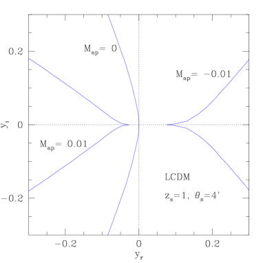
Figure 1: The integration path over the complex plane for the aperture-mass $M_{\rm ap}$ for the LCDM scenario, the source redshift $z_{s}=1$ and the angular radius $\theta_{s}=4^{\prime}$. We show the paths associated with $M_{\rm ap}=-0.01$ (right), $M_{\rm ap}=0$ (center) and $M_{\rm ap}=0.01$ (left). We clearly see that for large $|M_{\rm ap}|$ the integration path gets stucked onto one of the branch cuts of the generating function $\varphi_{\hat{M_{\rm ap}}}(y)$.

In order to compute the pdf ${\cal P}(\hat{X})$ from the inverse Laplace transform (37) we must perform the integration over $y$ in the complex plane. We choose the integration path so that the argument of the exponential in eq.(37) is a real negative number in order to avoid oscillations and to obtain a fast convergence. From the definition (36) it is clear that the generating function $\varphi_{\hat{X}}(y)$ obeys the symmetry $\varphi_{\hat{X}}(y^{*})=\varphi_{\hat{X}}(y)^{*}$, for any real observable $\hat{X}$ like the shear component $\gamma_{1s}$ or the aperture-mass $M_{\rm ap}$, so that the integration path over $y$ is symmetric with respect to the real axis. Moreover, we have to make sure that the integration path does not cross the branch cuts of $\varphi_{\hat{X}}(y)$. This implies that for large $|\hat{X}|$ the integration path is pinched on the real axis onto the singularities $y_{s,\hat{X}}^{\pm}$. This directly yields an exponential tail for the pdf ${\cal P}(\hat{X})$, as can be seen in a straightforward way from the expression (37). We discussed this point in more detail in Sect. 4.3 above. For illustration, we show in Fig. 1 the integration paths obtained for the aperture-mass in the LCDM case for $z_{s}=1$ and $\theta_{s}=4^{\prime}$. For $M_{\rm ap}=0$ the path runs through the origin $y=0$ while for large positive $M_{\rm ap}$ it gets stucked onto the negative branch cut of $\varphi_{\hat{X}}(y)$ (and similarly for large negative $M_{\rm ap}$).

4.6 Edgeworth expansion

As is well known, a centered Gaussian distribution is fully defined by its second order moment $\langle\hat{X}^{2}\rangle_{c}$. When the pdf ${\cal P}(\hat{X})$ deviates from the Gaussian all higher-order cumulants $\langle\hat{X}^{p}\rangle_{c}$ generically become non-zero and the pdf now depends on this whole series. Thus, in Sect. 4.1 and Sect. 4.2 we had to resum all these cumulants through the generating function $\varphi_{\hat{X}}(y)$ defined in eq.(36) in order to determine the pdf ${\cal P}(\hat{X})$ as in eq.(37). However, when the deviations from the Gaussian are small one can use the asymptotic Edgeworth expansion which describes the departures from the Gaussian encoded by the few lowest order cumulants. Let us define the parameters $S_{p}^{\hat{X}}$ associated with the variable $\hat{X}$ as in eq.(24):

$$\varphi_{\hat{X}}(y)=\sum_{p=2}^{\infty}\frac{(-1)^{p-1}}{p!}\;S_{p}^{\hat{X}}\;y^{p}\hskip 8.5359pt\mbox{with}\hskip 8.5359ptS_{p}^{\hat{X}}=\frac{\langle\hat{X}^{p}\rangle_{c}}{\langle\hat{X}^{2}\rangle_{c}^{p-1}}.$$ (65)

Here we assumed the random variable $\hat{X}$ to have zero mean ($\langle\hat{X}\rangle=0$) as is the case for weak lensing observables from eq.(15) since $\langle\delta\rangle=0$. Then, substituting the expansion (65) into eq.(37) and expanding the non-Gaussian part of the exponent one obtains (e.g., Bernardeau & Kofman 1995):

$${\cal P}(\hat{X}) = \frac{1}{\sqrt{2\pi\sigma_{\hat{X}}^{2}}}\;e^{-\nu^{2}/2}\;\Bigg{\{}1+\sigma_{\hat{X}}\frac{S_{3}^{\hat{X}}}{6}H_{3}(\nu)$$ (66)

$$+\sigma_{\hat{X}}^{2}\left[\frac{S_{4}^{\hat{X}}}{24}H_{4}(\nu)+\frac{(S_{3}^{\hat{X}})^{2}}{72}H_{6}(\nu)\right]+..\Bigg{\}}$$

with:

$$\sigma_{\hat{X}}=\langle\hat{X}^{2}\rangle_{c}^{1/2}\hskip 8.5359pt\mbox{and}\hskip 8.5359pt\nu=\frac{\hat{X}}{\sigma_{\hat{X}}}.$$ (67)

Here we introduced the Hermite polynomials $H_{n}(\nu)$. In particular we have:

$$H_{3}(\nu)=\nu^{3}-3\nu\hskip 8.5359pt\mbox{and}\hskip 8.5359ptH_{4}(\nu)=\nu^{4}-6\nu^{2}+3.$$ (68)

Since this is an asymptotic expansion, the Edgeworth expansion (66) is only useful for moderate deviations from the Gaussian, that is when the first correcting term is smaller than unity (typically $|\nu|\la 1$ and $|\sigma_{\hat{X}}S_{3}^{\hat{X}}|\la 1$), and the accuracy does not improve by including higher order terms in the expansion (66) (unless the pdf is extremely close to the Gaussian). The advantage of the Edgeworth expansion is that it provides a straightforward estimate of the pdf ${\cal P}(\hat{X})$ when it is still relatively close to the Gaussian, using only the skewness $S_{3}^{\hat{X}}$ or the kurtosis $S_{4}^{\hat{X}}$. This avoids the need to resum all higher-order cumulants and to perform the integration over the complex plane as in eq.(37).

5 The shear and aperture-mass statistics from numerical simulations

The numerical method for the computation of the lensing statistics is based on the original formalism of Couchman, Barber & Thomas, 1999, and which has been further developed by Barber, 2002. The original formalism allows for the computation of the three-dimensional shear matrices at a large number of locations within each $N$-body simulation volume output. In the present work we have evaluated the shear at 300 locations along every one of $455\times 455$ lines of sight in each of the simulation volumes. The development allows for the successive combination of these matrices along the lines of sight and throughout the linked simulation volumes from the sources at the required redshifts to the observer at $z=0$. The overall procedure therefore gives rise to Jacobian matrices for each line of sight and for each of the specified source redshifts from which the required lensing statistics have been generated.

Our procedure has been applied to two different cosmological simulations created by the Hydra Consortium using the ‘Hydra’ $N$-body hydrodynamics code (Couchman, Thomas & Pearce, 1995). The parameters describing the two cosmologies, LCDM and OCDM, are given in Table 1. Both contained $86^{3}$ dark matter particles of mass $1.29\times 10^{11}h^{-1}$ solar masses each, where $h$ is the value of the Hubble parameter expressed in units of 100 km s^-1 Mpc^-1. We used a variable particle softening within the code, to reflect the density environment of each particle, the minimum value of which, for particles in the densest environments, was chosen to be $0.0007(1+z)$ in box units, where $z$ is the redshift of the particular simulation volume.

Table 1: The parameters used in the two cosmological simulations. $\Omega_{\rm m}$ is the matter density parameter, $\Omega_{\Lambda}$ is the vacuum energy density parameter, $\Gamma$ is the power spectrum shape parameter, $\sigma_{8}$ is the normalisation on scales of $8h^{-1}$ Mpc, $\theta_{\rm res}$ is the angular resolution and $\theta_{\rm survey}^{2}$ is the angular size of the complete field of view throughout the simulations.

	$\Omega_{\rm m}$	$\Omega_{\Lambda}$	$\Gamma$	$\sigma_{8}$	$\theta_{\rm res}$	$\theta_{\rm survey}^{2}$
LCDM	0.3	0.7	0.25	1.22	$0^{\prime}.34$	$2^{\circ}.6\times 2^{\circ}.6$
OCDM	0.3	0.0	0.25	1.06	$0^{\prime}.37$	$2^{\circ}.8\times 2^{\circ}.8$

The angular resolution in the LCDM cosmology was $0^{\prime}.34$, equivalent to the minimum value of the particle softening at $z=0.36$, which is the redshift for the maximum lensing effects for sources at a redshift of 1 in that cosmology. In the case of the OCDM cosmology, the angular resolution was $0^{\prime}.37$. The angular size of the survey referred to in Table 1 corresponds to completely filling the front face of the redshift 1 simulation volume for an observer at redshift zero. For source redshifts greater than 1, the periodicity of the particle distributions was used to allow lines of sight beyond the confines of the simulation volumes to be included, as described in Barber, Munshi & Valageas, 2003.

The sources for our simulations were assumed to lie in a regular $455\times 455$ array at the front face of the simulation volume corresponding to the specified redshift. We used 14 different values for the source redshifts in each cosmology, whose exact redshift values are specified in Table 2. The redshifts selected were chosen to be close to redshifts of 0.1, 0.2, 0.3, 0.4, 0.5, 0.6, 0.7, 0.8, 0.9, 1.0, 1.5, 2.0, 3.0 and 3.5. In this paper the redshifts are referred to loosely as these approximate values, although in the determination of the lensing statistics, the actual redshift values were used.

Table 2: The redshifts of the sources in the two cosmologies.

	$z_{1}$	$z_{2}$	$z_{3}$	$z_{4}$	$z_{5}$	$z_{6}$	$z_{7}$	$z_{8}$	$z_{9}$	$z_{10}$	$z_{11}$	$z_{12}$	$z_{13}$	$z_{14}$
LCDM	0.10	0.21	0.29	0.41	$0.49$	$0.58$	0.72	0.82	0.88	.99	1.53	1.97	3.07	3.57
OCDM	0.11	0.18	0.31	0.41	$0.51$	$0.63$	0.69	-	0.88	1.03	1.47	2.03	3.13	3.53

Each of the simulation volumes had comoving side-dimensions of 100$h^{-1}$Mpc and to avoid obvious structure correlations, each was arbitrarily translated, rotated and reflected about each coordinate axis for each of the total of $N=10$ runs through all the volumes. In this way, we obtained $N$ sets of Jacobian matrices for the different runs.

By extracting the data needed from the Jacobians, the data for the shear components and convergence were smoothed on the different angular scales using a top-hat filter for the shear and the compensated filter for the aperture mass. To obtain the required pdfs and lower order moments the unsmoothed field in real space was convolved with the appropriate filters using the following scheme. Concentric annuli, separated equally in the radial direction, were used for sampling of the denisty field, as shown in figure 2. These annuli were than divided into equally spaced angular bins. The density field was computed along the radial and angular bins using a linear interpolation scheme from adjacent bins, before convolving it with the filters. Various combinations of the radial bin width and angular bin size were considered to check the convergence and numerical stability of the scheme. Our scheme enforces the radial symmetry inherent in the window functions which is important when dealing with window functions that have more features compared to a tophat filter. We have checked the stability by taking up to $20$ radial binning divisions for large smoothing radius and $60$ divisons along the angular directions. In addition, we have given random shifts to the rectangular grid along both axes to get a better sampling of the density field. We have also checked various levels of dilution by considering randomly selected points in the catalogue. In addition, we have checked various levels of uniform dilution where we choose uniformly spaced points to evaluate the statistics of the aperture mass, $M_{\rm ap}$. It became clear from our studies that grid effects will be much more pronounced in any statistical analysis related to compensated filters. This is due to the fact that for a given smoothing scale, compensated filters take more contributions from smaller angular scales.

Figure 2: Schematic description of the angular bins used for evaluation of $M_{ap}$ statistics.

Finally, the computed values for the pdfs, higher-order moments and aperture mass from each of the runs in each cosmology were averaged so that the errors on the means of $1\sigma/\sqrt{N}$ for each statistic were determined.

6 Results

Our study can be divided in two parts. In addition to the lower order moments we compute the complete pdf and we study their variation as a function of smoothing radius as well as their evolution with redshift. For the pdf of the aperture mass we investigate both the minimal tree model and the stellar model, which allows us to study the dependence on the detailed modeling of the correlation function (both models give close results for the shear).

6.1 The length scales probed by shear statistics

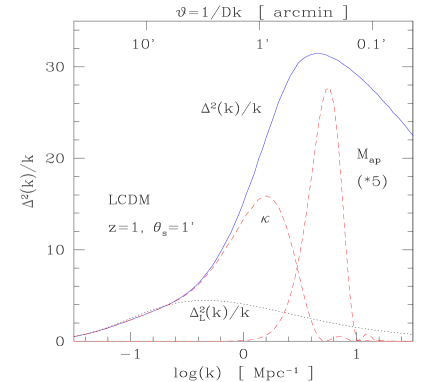
Figure 3: The contribution of various comoving wavenumbers $k$ to weak lensing observables at redshift $z=1$ along the line of sight. The solid line is the non-linear power $\Delta^{2}(k)/k$ (obtained from Peacock & Dodds 1996) while the dotted line is the linear power $\Delta^{2}_{L}(k)/k$ (i.e. using the linear power-spectrum). The left dashed line shows the contribution $W_{\kappa}(k_{\perp}{\cal D}\theta_{s})\Delta^{2}(k)/k$ to the variance of the smoothed convergence $\kappa_{s}$ (or to the smoothed shear component $\gamma_{1s}$) for the angular radius $\theta_{s}=1^{\prime}$. The right dashed line shows the contribution $W_{M_{\rm ap}}(k_{\perp}{\cal D}\theta_{s})\Delta^{2}(k)/k$, multiplied by a factor $5$, to the variance of the aperture-mass $M_{\rm ap}$ for $\theta_{s}=1^{\prime}$. The upper axis shows the angular scale $\vartheta=1/{\cal D}k$ associated to comoving wavenumber $k$.

As we study a range of source redshifts and smoothing angular scales the weak lensing observables (such as the shear or the aperture-mass) probe the density field over various length scales and redshifts, which run from the linear to the highly non-linear regime. The redshift dependence of the typical length scale comes from the angular diameter distance ${\cal D}(z)$, see eq.(26). The typical comoving wavenumber probed by various shear statistics for a smoothing angle $\theta_{s}=1^{\prime}$ are of the order of $1$ to $10h{\rm Mpc}^{-1}$ which corresponds to scales $0.1$ to $1h^{-1}$ Mpc, see Fig.5 in Barber, Munshi & Valageas (2003). In terms of the power per logarithmic wavenumber interval $\Delta^{2}(k)$, for $1^{\prime}<\theta_{s}<8^{\prime}$, this yields $0.1\la\Delta^{2}(k)\la 400$, see Fig.6 in Barber, Munshi & Valageas (2003). Hence most of the contribution to the weak lensing shear comes from intermediate length scales which cannot be described by the quasi-linear limit nor by the stable-clustering ansatz. As a consequence, in order to study weak lensing over the angular scales of interest for observational purposes (i.e. from $1^{\prime}$ up to $20^{\prime}$) one needs to use a model which can be applied from the quasi-linear regime up to the highly non-linear regime. The models which we recalled in Sect. 3 (see also Valageas, Barber & Munshi 2003 and Barber, Munshi & Valageas 2003 for details) provide such a tool and yield all properties of the density field (both the amplitude and the angular dependence of the many-body correlations) over the entire dynamical range.

We show in Fig. 3 the contribution of various comoving wavenumbers $k$ to weak lensing observables at redshift $z=1$ along the line of sight. We first plot the non-linear power $\Delta^{2}(k)/k$ (obtained from Peacock & Dodds 1996, solid line) and the linear power $\Delta^{2}_{L}(k)/k$ (i.e. using the linear power-spectrum, dotted line). Indeed, because of the projection associated with the integration along the line-of-sight, the power coming from a wavenumber $k$ to weak lensing observables is not $\Delta^{2}(k)$ (as for the 3-d density contrast $\delta_{R}$) but $\Delta^{2}(k)/k$, as seen from eq.(21). For CDM-like power-spectra, which flatten at small scales, we can see that the power $\Delta^{2}(k)/k$ decreases beyond $6$ Mpc^-1. Next, we show the contribution $W_{\kappa}(k_{\perp}{\cal D}\theta_{s})\Delta^{2}(k)/k$ to the variance of the smoothed convergence $\kappa_{s}$ (or to the smoothed shear component $\gamma_{1s}$) for the angular radius $\theta_{s}=1^{\prime}$ (left dashed line). At small wavenumbers it follows the power $\Delta^{2}(k)/k$ since $W_{\kappa}(0)=1$ and it exhibits a cutoff beyond $1/({\cal D}\theta_{s})$. The right dashed line is the contribution $W_{M_{\rm ap}}(k_{\perp}{\cal D}\theta_{s})\Delta^{2}(k)/k$ to the variance of the aperture-mass $M_{\rm ap}$ for the same angular radius $\theta_{s}=1^{\prime}$, multiplied by a factor 5 (for clarity on the figure). We can see that it probes a much narrower range of wavenumbers since the contribution from long wavelengths is suppressed because it involves a compensated filter with $W_{M_{\rm ap}}(0)=0$. Moreover, for the same angular radius we can check that $M_{\rm ap}$ probes higher wavenumbers than $\kappa_{s}$ because of this suppression of long wavelengths and of the profile of the filter which varies over scales $\sim\theta_{s}/4$. More precisely, from the upper axis which shows the angular scale $\vartheta=1/{\cal D}k$ associated with comoving wavenumber $k$, we see that the smoothed convergence or the smoothed shear mainly probe the density field at the wavenumber $k_{s}=1/{\cal D}\theta_{s}$ while contributions to the aperture-mass peak around $k_{s}=4/{\cal D}\theta_{s}$. This is why we chose the normalization (26) for the typical wavenumber $k_{s}$. Finally, the curves in Fig. 3 clearly show that the weak lensing signal comes from non-linear scales which cannot be described by the linear power $\Delta^{2}_{L}(k)/k$.

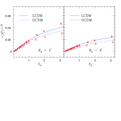
Figure 4: Variance of the smoothed shear component $\gamma_{is}$, $\langle\gamma_{is}^{2}\rangle^{1/2}$, as a function of the source redshift $z_{s}$. The smoothing angle $\theta_{s}$ is fixed at $1$ arcminute in left panel and at $4$ arcminute in the right panel. Lines correspond to the analytical prediction (21) and data points represent results from numerical simulations. Error bars are computed from scatter among various realizations. Variance of shear increases with source redshift $z_{s}$ for a fixed smoothing angle. Dots represent LCDM simulations whereas OCDM simulations are represented by open circles.

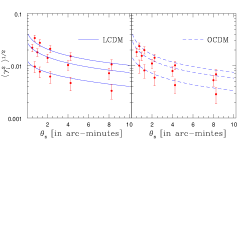
Figure 5: Variance is plotted as a function of smoothing angle for various fixed redshifts. Left panel correspond to LCDM and the right panel correspond to OCDM cosmology. The solid (LCDM) and dashed (OCDM) lines in each panels denote the analytical prediction (21) for the variance at redshifts $z_{s}=0.5,1$ and $1.5$ (from bottom to top). Points with error bars are numerical results from simulations.

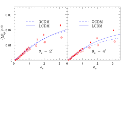
Figure 6: Variance plotted as a function of source redshift $z_{s}$. The aperture-mass compensated filter ($M_{\rm ap}$) is used to smooth the shear map. Left panel corresponds to smoothing angle $\theta_{s}=2^{\prime}$ and the right panel corresponds to $\theta_{s}=4^{\prime}$. The solid lines correspond to LCDM cosmology whereas the dashed lines correspond to OCDM cosmology. Data points represent averages of $10$ different realizations for each cosmology. Error bars are computed from scatter among various realizations. Dots represent LCDM simulations whereas OCDM simulations are represented by open circles.

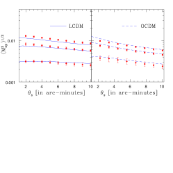
Figure 7: Aperture-mass variance plotted as a function of smoothing angle $\theta_{s}$. Left panel corresponds to LCDM cosmology whereas the right panel corresponds to OCDM cosmology. Three different redshifts are considered: $z_{s}=1.5,1$ and $z_{s}=0.5$ from top to bottom. Data points represent averages of $10$ different realizations for each cosmology. Error bars are computed from scatter among various realizations.

6.2 Variance of Shear and Aperture-Mass

We study the variance of smoothed shear components $\langle\gamma_{is}^{2}\rangle^{1/2}$ and aperture-mass $\langle M_{\rm ap}^{2}\rangle^{1/2}$ as a function of both source redshift $z_{s}$ and smoothing angle $\theta_{s}$ in Figs. 4-7. It follows the increase with redshift of the length of the line of sight. The variance is smaller in case of OCDM model mainly because of the smaller normalization $\sigma_{8}$. This implies that the LCDM pdfs are broader compared to OCDM pdfs for a given smoothing angle and a given redshift. As in the case of our convergence studies we have a reasonable agreement from the fitting formula of Peacock & Dodds (1996) over the entire range of redshift and smoothing angle. Our results agree with previous studies which focused on the variance of compensated filters (e.g., Hoekstra et al. (2002), van Waerbeke et al. (2002), Jarvis et al. (2003), Hamana et al. (2003), Benabed & van Waerbeke (2003)). However, we can see that at large redshifts and small scales, there appears to be some discrepancy between the analytic results and the simulations. This deviation shows the same behaviour for the shear and the aperture-mass but it is larger for the latter. We must point out that the computation of variance only depends on the two-point density correlation function (or the power spectrum) and not on the entire correlation hierarchy or the parameters $S_{p}$, which are the main focus of this paper. In other words, the deviations seen at large $z_{s}$ and small $\theta_{s}$ in Fig. 6 are solely due to the mismatch between the fit from Peacock & Dodds (1996) to the power spectrum and the numerical simulation. Therefore, they probably signal the effects of the finite numerical resolution (note that the softening length increases with $z$). On the other hand, it is known that the fit from Peacock & Dodds (1996) is not perfect (Smith et al. 2002).

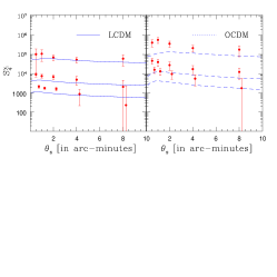
Figure 8: Kurtosis (see eq.(65) for definition) of the smoothed shear component $\gamma_{is}$, as a function of the smoothing angle $\theta_{s}$. The left panel corresponds to LCDM cosmology (solid lines) and the right panel to OCDM cosmology (dashed lines). Lines from top to bottom correspond to analytical predictions (57) (stellar model) for different source redshifts: $z_{s}=0.5,1$ and $1.5$. Points with error bars are the numerical results from simulations.

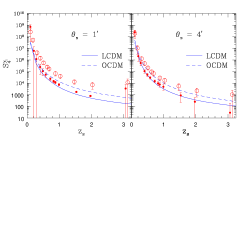
Figure 9: Kurtosis (see eq.(65) for definition) of the smoothed shear component $\gamma_{is}$ as a function of the source redshift $z_{s}$. The smoothing angle $\theta_{s}$ is fixed at $1$ arcminute in the left panel and at $4$ arcminute in the right panel. Lines correspond to the analytical prediction (57) (stellar model) and data points represent results from numerical simulations. Error bars are computed from scatter among various realizations. Although shear variance increases with redshift the kurtosis decreases with source redshift $z_{s}$. Black dots with error bars represent LCDM simulation while open circles represent OCDM simulations.

6.3 The Kurtosis of Shear

As pointed out in Sect. 2, for symmetry reasons all odd-order cumulants of shear components vanish. Therefore, the lowest-order non-Gaussian contribution is the kurtosis which we have studied as a function of both smoothing angle $\theta_{s}$ (Fig. 8) and source redshift $z_{s}$ (Fig. 9) (see also Takada & Jain 2002). We define the kurtosis as $S_{4}^{\gamma_{is}}=\langle\gamma_{is}^{4}\rangle_{c}/\langle\gamma_{is}^{2}\rangle^{3}$, as in eq.(65). We can check that we obtain a reasonable agreement with the numerical simulations. There is some discrepancy at small scales but this might be related to the numerical resolution. On the other hand, it is increasingly difficult to predict with a good accuracy higher-order moments of weak-lensing observables (or of the density field itself). In particular, while our model for the density field is in a sense “fitted” to the skewness $S_{3}$ of the density contrast through (25) (the quasi-linear limit $S_{3}^{\rm QL}$ is exact while the non-linear HEPT ansatz $S_{3}^{\rm NL}$ was seen to agree with numerical simulations), this is not the case for the kurtosis and higher-order moments of the density contrast. They are set by the simple parameterization of the generating function $\varphi(y)$ described in Valageas, Barber & Munshi (2003) and Barber, Munshi & Valageas (2003) which only depends on $S_{3}$. Moreover, in the case of weak-lensing observables there is a further dependence on the angular behaviour of the correlation functions. Thus, the minimal tree-model and the stellar model do not give identical results for the kurtosis (since the former writes the four-point correlation as a sum of a “stellar” and a “snake” diagram while the latter only keeps the “stellar” graph). Nevertheless, for the shear kurtosis both results are close and we only plot in Fig. 8 and Fig. 9 the stellar model prediction since it is this model which we shall investigate in more details in Sect. 6.5 for the full pdf because it is much more convenient for numerical purposes.

Note that whereas the variance of the shear components increases with the source redshift the kurtosis decreases. This is due both to the longer length of the line of sight (as we add the lensing contributions from successive mass sheets along the line of sight the total signal becomes closer to Gaussian, in agreement with the central limit theorem) and to the fact that the density field is closer to Gaussian at higher redshift. We can see that the variation with redshift of the kurtosis is actually very steep. This implies that any realistic observational study which aims to determine cosmological parameters from the lower-order moments of the shear components will have to determine source redshifts very accurately. On the other hand, the analytical calculations must take into account the spread of the distribution of source redshifts. This is actually straightforward within the formalism used in this article (see Valageas (2000a)) if we neglect non-linear couplings.

In realistic surveys one must also take into account the finite size of the catalog as well as the observational noise. A complete error analysis of higher-order moments for aperture-mass has been developed in Munshi & Coles (2002). Clearly from observational view points it is important to have a reasonable sky coverage and dense sampling of galaxies. Note that error analysis of lower order moments of shear components involves incorporating correlations among neighbouring cells which can be ignored for the study of aperture-mass statistics. This makes such studies for shear components more complicated although a crude order of magnitude study can be performed. It is also important to note that throughout we have ignored the noise due to intrinsic ellipticity distribution which we have to include in a more realistic study.

On the other hand, with future weak lensing surveys such as LSST and SNAP it will be feasible to study the non-Gaussianity induced by gravity with an unprecedented accuracy. It was pointed out by Hui (1999) that the skewness of the convergence field can directly be used to probe the dark energy equation of state. Future surveys with large sky coverage and dense sampling can also use the kurtosis of shear components to study the properties of dark energy. A clear detection of kurtosis will also help us to break the degeneracies in determining $\Omega_{\rm m}$ and $\sigma_{8}$ which are inherent in studies based on power spectrum analysis only (see also Takada & Jain 2002).

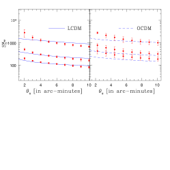
Figure 10: Skewness (see eq.(65) for definition) of the aperture-mass $M_{\rm ap}$ plotted as a function of smoothing angle $\theta_{s}$. Lines show the analytical prediction for $z_{s}=0.5,1$ and $z_{s}=1.5$ from top to bottom (the tree-model (44) and the stellar model (57) are identical for the skewness). Left panel corresponds to LCDM cosmology whereas the right panel corresponds to OCDM cosmology. Data points represent averages of $10$ different realizations for each cosmology. Error bars are computed from scatter among various realizations.

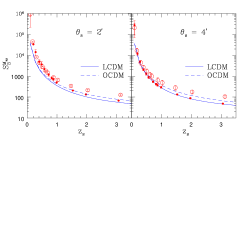
Figure 11: Skewness (see eq.(65) for definition) of the aperture-mass $M_{\rm ap}$ plotted as a function of source redshift $z_{s}$. The left panel corresponds to smoothing angle $\theta_{s}=2^{\prime}$ and the right panel corresponds to $\theta_{s}=4^{\prime}$. The solid lines in each panel correspond to LCDM cosmology whereas the dashed lines correspond to OCDM cosmology. Data points represent averages of $10$ different realizations for each cosmology. Error bars are computed from scatter among various realizations. Black dots corresponds to LCDM simulations whereas open circles correspond to OCDM simulations.

6.4 Skewness of Aperture-Mass

The shear kurtosis can be directly measured from shear maps hence it is a natural tool to study the departure from Gaussianity of the density field. However, as we noticed in Sect. 6.3 it suffers from several drawbacks. First, predictions for the kurtosis of the density field are less robust than for the skewness, which is a lower-order moment. Moreover, the relationship between the third-order moments of the density constrast and weak-lensing observables is stronger because the dependence on the angular behaviour of the correlation functions is smaller. Thus, all tree-models (including both the minimal tree-model and the stellar model studied in more details in this paper) give the same predictions for any statistics of order three (e.g., the skewness of the aperture-mass or any three-point correlation) since at this order there is only one tree graph, whose weight is fully defined by $S_{3}$. This makes the skewness of the aperture-mass $S_{3}^{M_{\rm ap}}$ the most useful probe of the non-Gaussianity of the density field. An additional advantage is that the aperture-mass provides a very localised probe of the density field in Fourier space, as seen in Fig. 3. This makes the comparison between theory and observations more robust and more precise as we can probe a narrow range of scales, hence a well-defined regime of gravitational clustering.

Therefore, we plot in Fig.10 and Fig. 11 the skewness $S_{3}^{M_{\rm ap}}$ as a function of smoothing angle $\theta_{s}$ and source redshift $z_{s}$. We again obtain a reasonable agreement between our theoretical predictions and the numerical simulations. Of course, like the kurtosis $S_{4}^{\gamma_{is}}$ of the shear the skewness decreases at higher redshifts. Note however that this variation is significantly shallower which is a useful property for observational purposes (the error introduced by the measure of the source redshifts will be smaller).

Although present generation surveys do not provide a clear cosmological signal for non-zero skewness, future surveys such as Supernova Anisotropy Probe (SNAP) and the Large-aperture Synoptic Survey Telescope (LSST) will be very useful in this direction. On the other hand, various generalizations of the skewness $S_{3}^{M_{\rm ap}}$ have been proposed recently along with fast computational techniques which can reduce large volumes of data delivered by future weak lensing surveys. These generalisations can also handle decomposition into cosmological modes and non-gravitational modes induced by systematics (see e.g. Jarvis, Bernstein & Jain 2003).

Our studies are complimentary to other works which have focused on constraining or determining various halo model parameters from such observational studies. Our approach is significantly different as it is based on the many-body correlations of the density field themselves, rather than relying on a decomposition of the matter distribution over a population of virialized halos.

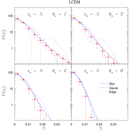
Figure 12: Probability distribution function ${\cal P}(\gamma_{is})$ of the smoothed shear component $\gamma_{is}$. The smoothing angle $\theta_{s}$ is mentioned in each panel while the underlying cosmological parameters are that of LCDM. The sources are all placed at the same redshift $z_{s}=0.5$. Since the pdf is even (${\cal P}(\gamma_{is})={\cal P}(-\gamma_{is})$) we only display the pdf for positive $\gamma_{is}$. Solid lines correspond to the analytical prediction (59) of the stellar model. The dashed lines show the Gaussian distribution with the same variance. The dotted lines correspond to the inclusion of the first non-zero term (kurtosis) in the Edgeworth expansion beyond the Gaussian approximation, eq.(66). Data points are results from numerical simulations. Error bars indicate the scatter among various realizations.

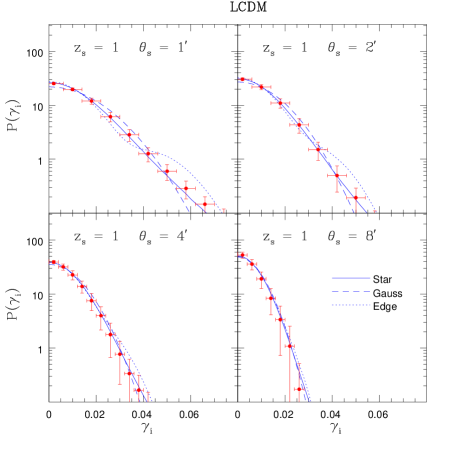
Figure 13: As in previous figure but for source redshift $z_{s}=1$. Note that as we move towards higher redshifts the distribution becomes more Gaussian and the Edgeworth expansion matches the analytical expression better. However, truncating the expansion at any order produces spurious oscillations which are not physical.

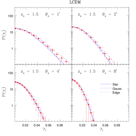
Figure 14: As in previous figure but for source redshift $z_{s}=1.5$.

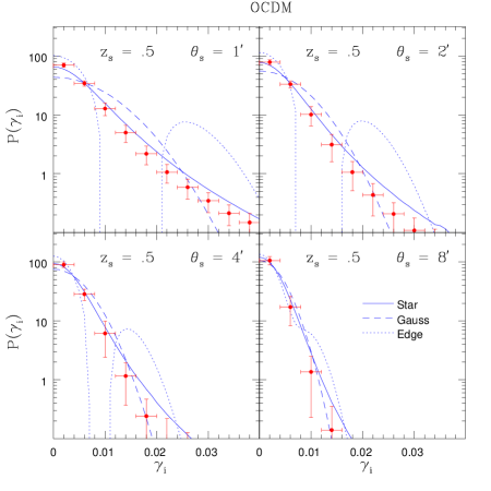
Figure 15: As in previous figure but for source redshift $z_{s}=0.5$ and the OCDM cosmology.

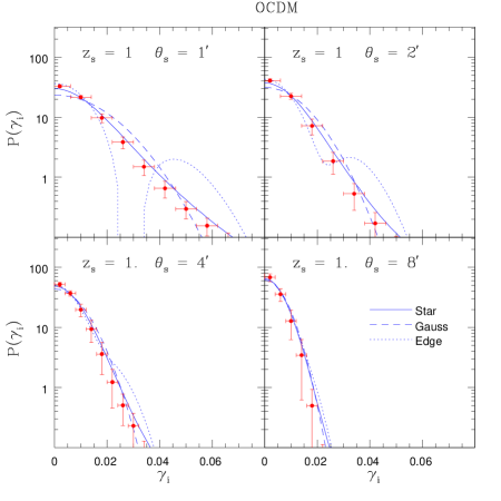
Figure 16: As in previous figure but for source redshift $z_{s}=1$.

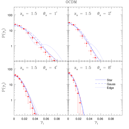
Figure 17: As in previous figure but for source redshift $z_{s}=1.5$.

6.5 Probability Distribution Function for Shear Components $\gamma_{is}$

Our analytical results provide a complete analytical modeling of the pdf of shear components. Extending our earlier studies (Valageas, Barber & Munshi 2003) we show that indeed such a description is possible for the entire range of redshifts as well as smoothing angles of practical interest. Thus, we compare with numerical simulations our analytical predictions for the pdf ${\cal P}(\gamma_{is})$ of the smoothed shear components in Figs. 12 - 17. We consider both LCDM and OCDM cosmologies, for smoothing angles $\theta_{s}=1^{\prime},2^{\prime},4^{\prime}$ and $8^{\prime}$ and for three different source redshifts $z_{s}=0.5,1$ and $1.5$. We can see that we obtain a good agreement over the entire range of smoothing radius and source redshift, from linear to highly non-linear scales. We only plot the prediction of the stellar model (59) because it is much more convenient for practical purposes. Indeed, eq.(59) provides a simple explicit expression for the generating function $\varphi_{\gamma_{is}}(y)$. By contrast, the minimal tree-model yields an implicit system (53)-(54) which must be solved numerically at each point $y$. Since the variable ${\vec{\vartheta}}$ is actually two-dimensional this involves solving for a 2-d function $\tau({\vec{\vartheta}})$ defined as the fixed point of eq.(54). This cannot be done by a simple iterative procedure for arbitary $y$ since it would diverge for large $y$. Therefore, this implies the use of a time-consuming algorithm. Note that the generating function $\varphi_{\gamma_{is}}(y)$ must then be integrated over the complex plane in eq.(37). Thus, the stellar model is much simpler to implement and since both models give close predictions for the shear we focus on the stellar model in Figs. 12 - 17. Note that we have already shown in Barber, Munshi & Valageas (2003) that both models also give almost identical predictions for the smoothed convergence $\kappa_{s}$.

We also plot the Gaussian (dashed line) and the Edgeworth expansion (dotted line) up to the first non-Gaussian correction (here the kurtosis) from eq.(66). We can check that at large smoothing angles $\theta_{s}$ and source redshifts $z_{s}$ the pdf ${\cal P}(\gamma_{is})$ becomes very close to Gaussian. This could already be expected from the behaviour of the kurtosis analysed in Sect. 6.3. The departure from the Gaussian is significant at $z_{s}\sim 0.5$ and $\theta_{s}\la 2^{\prime}$. On the other hand, we note that the Edgeworth expansion is actually useless. It only provides reasonable results when the pdf is very close to Gaussian while as soon as there is a sizeable deviation from the Gaussian it introduces spurious oscillations and it actually fares worse than the Gaussian. Note that since it is an asymptotic expansion including higher-order terms would further worsen this discrepancy.

One of the benefits of being able to study the shear components analytically is to have a means to cross check the effects of various systematics which go into the making of convergence maps from shear data. Alternatively one can work with compensated filters to construct the $M_{\rm ap}$ statistics as described above. Similarly, in a previous paper (Valageas, Barber & Munshi 2003) we have shown that not only the statistics of the shear components can be modeled in this manner but one can also derive the properties of the shear modulus $|\gamma_{s}|$. However, we found that the correlation between the two components is almost negligible so that the pdf of the shear modulus does not carry useful additional information. This is the reason why we have not included ${\cal P}(|\gamma_{s}|)$ in the present study although it is a simple outcome of the analytical results presented here.

Since the pdf ${\cal P}(\gamma_{is})$ contains some information about the entire hierarchy of the $S_{p}^{\gamma_{is}}$ cumulants it can be used as a probe of the entire pdf of the underlying mass distribution. This is clearly apparent in eq.(59). Moreover, it may be used to distinguish cosmological models in a more efficient manner than relying on the few lowest-order moments. Given that the shear maps are a direct outcome of any weak lensing survey, we may hope that surveys with a low level of noise as well as a good sky coverage could give us some clues on the distribution of matter in addition to the cosmological parameters. However, we see in Figs. 12 - 17 that the pdf ${\cal P}(\gamma_{is})$ is not very far from the Gaussian, partly because it is even so that the shape is roughly similar, hence it may be difficult to extract accurate measures from future surveys.

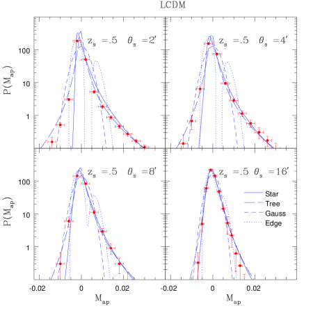
Figure 18: Probability distribution function ${\cal P}(M_{\rm ap})$ for the $M_{\rm ap}$ statistic which uses a compensated filter. We probe various smoothing radii from $\theta_{s}=2^{\prime}$ up to $\theta_{s}=16^{\prime}$. All sources are placed at source redshift $z_{s}=0.5$ and we consider the LCDM cosmology. Solid lines show the prediction of the stellar model (59). Long dashed lines correspond to the minimal tree-model (53)-(54). Short dashed lines are the Gaussian with the same variance while the dotted lines are the Edgeworth expansion (66) including the first correction to Gaussianity (skewness). Data points are results from numerical simulations. Ten different realizations are analysed and error bars denote the scatter among various realizations. Note that for negative $M_{\rm ap}$ the minimal tree-model predictions are much closer to numerical simulations than the stellar model.

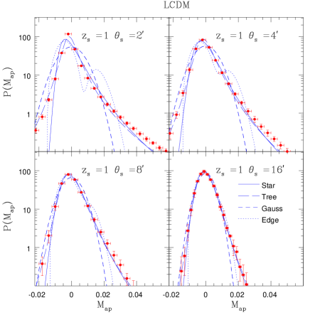
Figure 19: As in previous figure but for source redshift $z_{s}=1$.

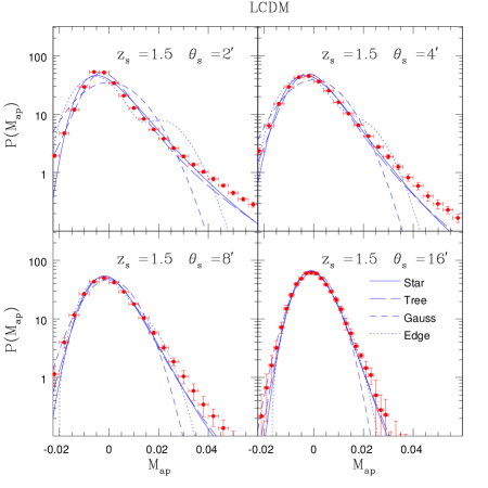
Figure 20: As in previous figure but for source redshift $z_{s}=1.5$.

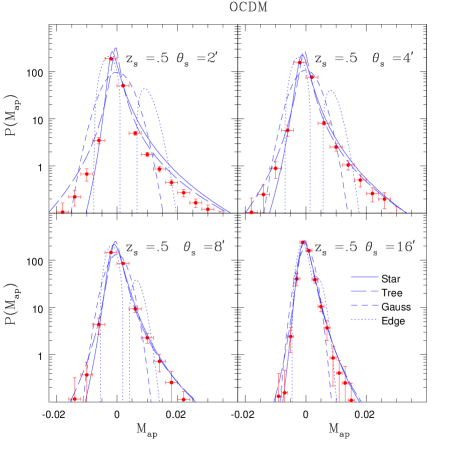
Figure 21: As in previous figure but for source redshift $z_{s}=0.5$ and the OCDM cosmology.

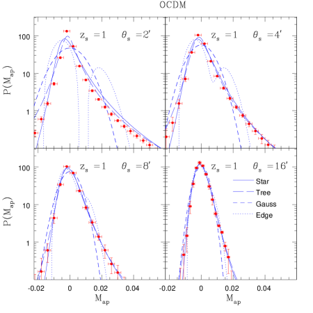
Figure 22: As in previous figure but for source redshift $z_{s}=1$.

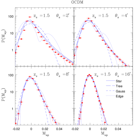
Figure 23: As in previous figure but for source redshift $z_{s}=1.5$.

6.6 Probability Distribution Function for Aperture-Mass

As discussed in Sect. 6.4, the aperture-mass $M_{\rm ap}$ shows several advantages over the shear components $\gamma_{is}$. In particular, it probes a narrower range of scales and it is not an even quantity. Therefore, we plot in Figs. 18 - 23 the pdf ${\cal P}(M_{\rm ap})$ of the aperture-mass. We again consider both LCDM and OCDM cosmologies and sources redshifts $z_{s}=0.5,1$ and $1.5$. However, we now study the smoothing angles $\theta_{s}=2^{\prime},4^{\prime},8^{\prime}$ and $16^{\prime}$. Indeed, as shown in Fig. 3 the aperture-mass probes smaller scales than the shear for a same angular radius, hence the limitation from the finite resolution of numerical simulations shifts to larger angles. On the other hand, we now plot the analytical predictions of both the minimal tree-model (53)-(54) (long dashed lines) and the stellar model (59) (solid lines). Indeed, contrary to the convergence (see Barber, Munshi & Valageas 2003) or the shear, the predictions of both models significantly differ at smaller angular scales for the large negative $M_{\rm ap}$ tail. As explained in Sect. 4.4, this behaviour can be understood on simple theoretical grounds. At very small angles ($\theta_{s}\la 0.4^{\prime}$) the pdf ${\cal P}(M_{\rm ap})$ predicted by the stellar model shows a singular behaviour and it vanishes for $M_{\rm ap}<0$. At the scales of pratical interest displayed in Figs. 18 - 23 the pdf is still regular but we can see a hint of the trend towards this singularity as the falloff at negative $M_{\rm ap}$ becomes increasingly steep for smaller scales. By contrast, the pdf obtained from the minimal tree-model which does not suffer from this singular behaviour shows a smoother cutoff at negative $M_{\rm ap}$ (although it remains sharper than for positive $M_{\rm ap}$, in agreement with numerical simulations). Note that this behaviour shows that no realizable density field can exactly obey the stellar model (whatever the coefficients $S_{p}$), while this remains an open question for the minimal tree-model.

We can see in the figures that the prediction from the minimal tree-model shows a good agreement with the numerical simulations over all scales and redshifts of interest. On the other hand, as expected from the previous discussion the stellar model fails to reproduce the tail at negative $M_{\rm ap}$, except for large angles and redshifts. However, it yields a reasonable prediction for the pdf for $M_{\rm ap}>0$ (albeit the minimal tree-model fares slightly better in this domain too). Therefore, we can conclude that the minimal tree-model is a much better tool to study the statistics of the aperture-mass. Fortunately, although the numerical computation is still more difficult and more computer time consuming than for the stellar model, the function $\tau({\vec{\vartheta}})=\tau(\vartheta)$ introduced in eq.(54) is now only one-dimensional which makes the computation much easier than for the shear (where $\tau({\vec{\vartheta}})$ was truly 2-dimensional), since the filter $U_{M_{\rm ap}}({\vec{\vartheta}})$ obeys a radial symmetry.

We also display the Gaussian (dashed lines) with the same variance. Of course, at large redshifts and angles the pdf becomes closer to Gaussian but we can see that even for $\theta_{s}\sim 8^{\prime}$ and $z_{s}\sim 1.5$ the deviations from Gaussianity are clear. Moreover, at smaller angles and redshifts the Gaussian completely fails to reproduce the pdf obtained from numerical simulations. It cannot follow the sharp peak at $M_{\rm ap}\simeq 0$, the extended tails and the asymmetry of the pdf. Thus, we can see that the departure from Gaussianity is much more important for ${\cal P}(M_{\rm ap})$ than for the pdf ${\cal P}(\gamma_{is})$ of the shear studied in Sect. 6.5. Therefore, the pdf ${\cal P}(M_{\rm ap})$ of the aperture-mass should provide a much more efficient tool to measure the deviations from Gaussianity than the pdf ${\cal P}(\gamma_{is})$ of the shear. Note that non-Gaussian features, like low-order moments for instance, exhibit a strong $\Omega_{\rm m}$-dependence, mainly due to the presence of the normalising factor in eq.(1) (e.g., Bernardeau et al. 1997). Therefore, the aperture-mass is a convenient tool to measure such cosmological parameters as well as the properties of the underlying density field. On the other hand, we also plot the Edgeworth expansion (dotted lines) up to the first non-Gaussian term (skewness). As was the case for the shear, we can see that this asymptotic expansion is of very little use, since it only fares well at large angles and redshifts where the Gaussian is already a reasonable description (although it somewhat improves the shape of the pdf near its maximum) while as soon as there is a significant deviation from the Gaussian it yields spurious oscillations which make it useless (in some domains it even gives negative values for ${\cal P}(M_{\rm ap})$).

Attempts in modeling the pdf ${\cal P}(M_{\rm ap})$ were initiated by Reblinsky et al. (1999), where a halo model of clustering was assumed in order to compute the positive tail of the pdf. Indeed, the high-$M_{\rm ap}$ tail is very efficient in probing and mapping out large concentrations of dark mass in weak lensing surveys. On the other hand, a complete prediction of the pdf for all values of $M_{\rm ap}$, which would be difficult to obtain from a halo model which cannot faithfully describe low-density regions and filamentary structures, gives a valuable insight in probing both overdense and underdense regions in a statistical manner. We have shown that our method, which is based on the many-body correlations rather than on a decomposition over halos, provides such a model. In particular, the results presented above show that the negative $M_{\rm ap}$-tail is very sensitive to the angular behaviour of the correlation functions (in addition to their amplitude). Therefore, it provides a direct probe of higher order correlations and it can help us to discriminate among various models of gravitational clustering. In fact, we have shown that it already rules out the stellar model even though this model provides a very good description for the statistics of the convergence (Barber, Munshi & Valageas 2003) and the smoothed shear (Sect. 6.5).

Our results extend the work by Bernardeau & Valageas (2000) who presented a detailed study of the pdf ${\cal P}(M_{\rm ap})$ within both the quasi-linear regime (where exact calculations are possible) and the highly non-linear regime (where they used the minimal tree-model). They also compared the predictions of the minimal tree-model with numerical simulations for various cosmologies, with $z_{s}=1$ and $\theta_{s}=4^{\prime}$. Here we have shown that the minimal tree-model actually provides good predictions for ${\cal P}(M_{\rm ap})$ over all scales and redshifts of interest, from quasi-linear to highly non-linear scales. Moreover, by introducing the stellar model we have shown that ${\cal P}(M_{\rm ap})$ could be used to probe the detailed angular behaviour of the many-body correlations in addition to their amplitude. A more complete study of ${\cal P}(M_{\rm ap})$ with realistic source distributions as well as noise due to the intrinsic ellipticity distribution will be presented elsewhere.

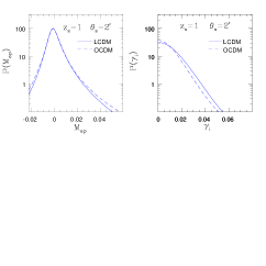
Figure 24: Probability distribution functions ${\cal P}(\gamma_{is})$ of the smoothed shear component $\gamma_{is}$ (right panel) and ${\cal P}(M_{\rm ap})$ for the $M_{\rm ap}$ (left panel) are compared for two different cosmologies for a given smoothing angle $\theta_{s}=2^{\prime}$ and source redshift $z_{s}=1$. Solid lines correspond to LCDM cosmology and dashed lines correspond to OCDM cosmology.

6.7 Comparison of the Probability Distribution Functions obtained for both cosmologies

Finally, for the sake of completeness, we plot in Fig. 24 the pdfs obtained in both cosmological models for the shear and the aperture-mass. The difference between both models is rather small. Indeed, these weak-lensing observables are mostly sensitive to the matter density parameter $\Omega_{\rm m}$ and to the amplitude $\sigma_{8}$ of the density fluctuations while the dependence on $\Omega_{\Lambda}$ is smaller. However, note that the comparison is not so straightforward since both $\Omega_{\Lambda}$ and $\sigma_{8}$ differ between the two models (and most of the change of the pdf comes from $\sigma_{8}$). A more precise study of the dependence on cosmological parameters and on the source redshift is left for future works.

7 Discussion

Weak lensing surveys are being regularly used to probe the matter distribution and the underlying cosmology. However, the modeling of statistical quantities related to weak lensing surveys, such as convergence maps or related shear maps, is rather difficult because of the non-linear nature of the underlying density field they try to probe. Besides, the non-linearity grows at smaller angular scales which should dominate the signal in forthcoming surveys. In a series of recent papers we have shown how to combine a widely used parameterization of the non-linear matter power-spectrum with various simple models of the matter density correlation hierarchy. This allows a detailed description of weak lensing statistics.

In the present paper we mainly focus on the statistical properties of the weak lensing shear components $\gamma_{is}$ and the closely related aperture-mass $M_{\rm ap}$. These two quantities can be computed from observational surveys in a direct manner from galaxy ellipticities (in the weak lensing regime). By contrast, extracting convergence maps is more difficult as it involves a non-local inversion problem and exhibits a mass sheet degeneracy. However, we must note that the measure of shear statistics still remains a difficult task because of the non-trivial survey topology (a fraction of the survey area has to be excluded from the analysis because of image defects, bright stars,..). Thus, rather than computing the shear or the aperture-mass realized over many complete circles on the sky, one usually estimates low-order correlation functions of the shear which are next integrated in order to obtain low-order moments of the smoothed shear or aperture-mass. However, we do not study these points in this article. We investigate two simple analytical descriptions of the matter density field: the minimal tree model and the stellar model which we introduced in Valageas, Barber & Munshi (2004). Both models give identical results for the statistics of the 3-d density contrast smoothed over spherical cells and only differ by the detailed angular dependence of the many-body density correlations.

In a previous study (Barber, Munshi & Valageas 2004) we have shown that both models also give almost identical results for the smoothed convergence $\kappa_{s}$. In agreement with earlier works, this shows that the pdf ${\cal P}(\kappa_{s})$ (or its moments) provides a robust measure of the pdf ${\cal P}(\delta_{R})$. This also enables one to measure in a robust fashion the underlying cosmological parameters as well as the amplitude of the density correlations. In the present study we extend such calculations to more intricate compensated filters which can directly be constructed from shear maps: the smoothed shear components $\gamma_{is}$ and the aperture-mass $M_{\rm ap}$. As these observables involve more intricate filters we can expect the dependence on the angular behaviour of the many-body correlations to be larger than for the smoothed convergence. We find that both models actually yield rather close results for the smoothed shear components and the positive tail of the aperture-mass. Moreover, we obtain a good agreement with numerical simulations over all scales and redshifts of practical interest. Therefore, in this domain the shear and the aperture-mass provide again a robust constraint on cosmological parameters and the statistics of the smoothed 3-d density contrast $\delta_{R}$. Besides, we found that ${\cal P}(M_{\rm ap})$ shows a stronger departure from the Gaussian than ${\cal P}(\gamma_{is})$, so that the aperture-mass appears to be a very useful tool in this respect.

On the other hand, we also note that at small angles ($\theta_{s}\la 2^{\prime}$) the tail of the pdf ${\cal P}(M_{\rm ap})$ for negative $M_{\rm ap}$ shows a strong variation between both models. Whereas the minimal tree-model provides a good description of the numerical data down to the smallest scales available to us the stellar model shows a significant discrepancy (while the part of the pdf over $M_{\rm ap}>0$ remains reasonable). The stellar model actually breaks down at $\theta_{s}\la 0.4^{\prime}$ for $M_{\rm ap}<0$. This clearly indicates that the aperture-mass statistics can be used as a very precise probe of the high-order correlation hierarchy. Contrary to the smoothed convergence $\kappa_{s}$, it is not only sensitive to the amplitude of the many-body correlations but also to their detailed angular behaviour. Thus, it provides a complimentary tool to the smoothed convergence or shear components. From a theoretical point of view, we can note that this behaviour also means that no physical density field can be exactly described by the stellar model (while this remains an open issue for generic minimal tree-models) although it provides a very interesting and convenient approximation which works very well for both the smoothed convergence and the smoothed shear components. This shows that the shape of the pdf ${\cal P}(M_{\rm ap})$ can actually rule out sensible models of gravitational clustering.

Combined with our previous results for shear and convergence statistics (Valageas, Barber & Munshi 2004, Barber, Munshi & Valageas 2004) we have developed a very powerful technique to analyse weak lensing survey results. Although in our present calculations (both analytical and numerical) we have not included observational details like the finite width in source distribution or the noise due to the intrinsic ellipticity distribution of galaxies, they can be incorporated easily in our computations. A detailed and more elaborate comparison will be presented elsewhere when such simulations become available.

Several interesting numerical issues became clear from our study. For a given angular scale $\theta_{s}$ compensated filters like $U_{M_{\rm ap}}$ pick up more contributions from higher wavenumbers as compared with tophat filters. This makes them more difficult to study numerically at smaller angular scales, as the finite resolution of the simulations starts to play a role. This is also the regime where $M_{\rm ap}$ statistics are very sensitive to the detailed analytical modeling of the correlation hierarchy. Our work serves as a precurser to studies using simulations with much finer resolutions. However, using such compensated filters also means that finite volume effects are much less pronounced as compared with tophat filters (see Munshi & Coles (2002) for a detailed analysis of various spurious results in determination of $M_{\rm ap}$ statistics).

Most analytical studies in the non-linear regime use a halo model (for detailed predictions of a halo model see Takada & Jain 2003). In principles, halo models (see Cooray & Sheth 200 for a review) can predict the higher-order correlation functions in the highly non-linear regime. Indeed, on small scales the latter are set by the density profile of the halos as the $p-$point correlations are dominated by the contribution associated with all $p$ points being within the same halo. However, it is interesting to note that the neglect of substructures may lead to larger inaccuracies for high-order statistics. On the other hand, at intermediate scales one also probes the correlations among different halos which introduces new unknowns and makes explicit calculations cumbersome. This is important for handling projection effects which involve the mixing of various scales. Finally, such a model for the density field is not well-suited to describe the low-density and underdense regions (e.g., voids, filaments) which are outside virialized objects. Our method follows a completely different approach based on the high-order correlation functions themselves rather than on a decomposition of the matter distribution over a population of virialized halos. Clearly such an approach provides an independent complimentary scheme and will be useful for various numerical cross-checks.

The simulation technique that we employ is completely different from the more popular ray tracing methods. Our studies therefore not only provide a good test for analytical results but it is also a good consistency test for such new simulation techniques.

References

- [1] Babul A., Lee M.H., 1991, MNRAS, 250, 407
- [2] Barber A. J., MNRAS, 2002, 335, 909
- [3] Barber A. J., Munshi D., Valageas P., MNRAS, 2004,347, 667
- [4] Barber A. J., Taylor A. N., 2003, MNRAS, 344, 789
- [5] Barber A. J., Thomas P. A., Couchman H. M. P. & Fluke C. J., 2000, MNRAS, 319, 267
- [6] Bacon D.J., Refregier A., Ellis R.S., 2000, MNRAS, 318, 625
- [7] Bernardeau F., Schaeffer R., 1992, A&A, 255, 1
- [8] Bernardeau F., Kofman L., 1995, ApJ, 443, 479
- [9] Bernardeau F., Valageas P., 2000, A&A, 364, 1
- [10] Bernardeau F., Van Waerbeke L., Mellier Y., 1997, A&A, 322, 1
- [11] Bernardeau F., Mellier Y., Van Waerbeke L., 2002, A&A, 389, L28
- [12] Colombi S., Bouchet F.R., Schaeffer R., 1995 ApJS, 96, 401
- [13] Couchman H. M. P., Barber A. J., Thomas P. A., 1999, MNRAS, 308, 180
- [14] Couchman H. M. P., Thomas P. A., Pearce F. R., 1995, Ap. J., 797
- [15] Cooray A., Sheth R., Phys.Rept. 372 (2002) 1
- [16] Fry J.N., 1984, ApJ, 279, 499
- [17] Groth E., Peebles P.J.E., 1977, ApJ, 217, 385
- [18] Gunn J.E., 1967, ApJ, 147, 61
- [19] Hamilton A.J.S., Kumar P., Lu E., Matthews A., 1991, ApJ, 374, L1
- [20] Hoekstra H., Yee H. K. C., Gladders M. D., 2002, ApJ, 577, 595
- [21] Hui L., 1999, ApJ, 519, 622
- [22] Jain B, 2002, ApJ., 580, L3
- [23] Jain B., Seljak U., 1997, ApJ, 484, 560
- [24] Jain B., Van Waerbeke L., 1999, astro-ph/9910459
- [25] Jain B., Seljak U., White S.D.M., 2000, ApJ, 530, 547
- [26] Jannink G., Des Cloiseaux J., 1987, Les polymères en solution, Les editions de physique, Les Ulis, France
- [27] Jaroszyn’ski M., Park C., Paczynski B., Gott J.R., 1990, ApJ, 365, 22
- [28] Kaiser N., 1992, ApJ, 388, 272
- [29] Kaiser N., 1998, ApJ, 498, 26
- [30] Limber D.N., 1954, ApJ, 119, 665
- [31] Munshi D., Bernardeau F., Melott A.L., Schaeffer R., 1999, MNRAS, 303, 433
- [32] Munshi D., Coles P., Melott A.L., 1999a, MNRAS, 307, 387
- [33] Munshi D., Coles P., Melott A.L., 1999b, MNRAS, 310, 892
- [34] Munshi D., Melott A.L., Coles P., 1999, MNRAS, 311, 149
- [35] Munshi D., Coles P., 2000, MNRAS, 313, 148
- [36] Munshi D., Coles P., 2002, MNRAS.329, 797
- [37] Munshi D., Coles P., 2003, MNRAS, 338, 846
- [38] Munshi D., Jain B., 2000, MNRAS, 318, 109
- [39] Munshi D., Jain B., 2001, MNRAS, 322, 107
- [40] Munshi D., 2000, MNRAS, 318, 145
- [41] Munshi D., Wang Y., 2003, ApJ, 583, 566
- [42] Navarro J.F., Frenk C.S., White S.D.M., 1996, ApJ, 462, 563
- [43] Peebles P.J.E., 1980, The large scale structure of the universe, Princeton University Press
- [44] Peacock J.A., Dodds S.J., 1996, MNRAS, 280, L19
- [45] Peacock J. A., Smith R. E., 2000, MNRAS, 318, 1144
- [46] Schaeffer R., 1984, A&A, 134, L15
- [47] Schneider P., Ehlers J., Falco E. E., 1992, ‘Gravitational Lenses,’ Springer-Verlag, ISBN 0-387-97070-3
- [48] Schneider P., Weiss A., 1988, ApJ, 330,1
- [49] Schneider P., 1996, MNRAS, 283, 837
- [50] Schneider P., Van Waerbeke L., Jain B., Kruse G., 1998, MNRAS, 296, 873, 873
- [51] Scoccimarro R., Colombi S., Fry J.N., Frieman J.A., Hivon E., Melott A.L., 1998, ApJ, 496, 586
- [52] Scoccimarro R., Frieman J.A., 1999, ApJ, 520, 35
- [53] Seljak U., 2000, MNRAS, 318, 203
- [54] Smith R. E. et al., 2003, MNRAS, 341, 1311
- [55] Stebbins A., 1996, astro-ph/9609149
- [56] Szapudi I., Szalay A.S., 1993, ApJ, 408, 43
- [57] Szapudi I., Szalay A.S., 1997, ApJ, 481, L1
- [58] Takada M., Jain B. 2002, MNRAS 337, 875
- [59] Valageas P., 1999, A&A, 347, 757
- [60] Valageas P., 2000a, A&A, 354, 767
- [61] Valageas P., 2000b, A&A, 356, 771
- [62] Valageas P., 2002, A&A, 382, 412
- [63] Valageas P., Barber A. J., Munshi D., 2004, MNRAS, 347,654
- [64] Van Waerbeke L., Bernardeau F., Mellier Y., 1999, A& A, 342, 15 Bernardeau F., 2001, MNRAS, 322, 918
- [65] Van Waerbeke L., Mellier Y., Pelló R., Pen U.-L., McCracken H. J., Jain B., 2002, A&A, 393, 369
- [66] Villumsen J.V., 1996, MNRAS, 281, 369
- [67] Wambsganss J., Cen R., Ostriker J.P., 1998, ApJ, 494, 298 29 1995, Science, 268, 274
- [68] Wang Y., Holz D. E., Munshi D., 2002, ApJ, 572L, 15