Signatures of Magnetized Large Scale Structure in Ultra-High Energy Cosmic Rays

Abstract

We investigate the impact of a structured universe in the multi-pole moments, auto-correlation function, and cluster statistics of cosmic rays above $10^{19}\,$eV. We compare structured and uniform source distributions with and without magnetic fields obtained from a cosmological simulation. We find that current data marginally favor structured source distributions and magnetic fields reaching a few $\mu$G in galaxy clusters but below $0.1\,\mu$G in our local extragalactic neighborhood. A pronounced GZK cutoff is also predicted in this scenario. Future experiments will make the degree scale auto-correlation function a sensitive probe of micro Gauss fields surrounding the sources.

Introduction: The origin and nature of ultra high energy cosmic rays (UHECRs) is one of the most puzzling problems of high energy astrophysics bs-rev . Beside the actual mechanism responsible for the acceleration of the particles to energies as high as a few $\times 10^{20}\,$eV and more, propagation of UHECRs in intergalactic space is a delicate and critical part of the full investigation. It was soon recognized that energy losses dramatically limit the possible distance traveled by these particles; in particular, interactions with cosmic microwave background photons lead to catastrophic photo-meson production at energies above $\sim 5\times 10^{19}\,$eV, the GZK effect gzk . Charged nucleons are also susceptible to deflections induced by extragalactic magnetic fields (EGMF). The importance and the subtlety of the effects produced by this process have been emphasized by a number of authors sigletal ; sse ; ynts ; tanco . However, up to date, the properties of EGMF are only very poorly constrained; therefore, their impact on the propagation of UHECRs is still quite uncertain and a number of different scenarios, compatible with the available observational constraints, must be investigated.

Along this line of reasoning, recently we have investigated UHECR propagation in a highly structured EGMF obtained from a simulation of large scale structure formation sme . The EGMF was evolved according to the induction equation. Its seeds were generated at shocks in accord to the Biermann battery mechanism kcor97 . Thus, it was amplified in different parts of the universe according to the velocity field provided by the simulated gas component. Lorentz forces were neglected as EGMF are known to be dynamically unimportant in most of the universe volume. The resulting field strength was normalized so as to reproduce observed rotation measure values in galaxy clusters bo_review . The EGMF are significant only within filaments and groups/clusters of galaxies. The relative strength there and the resulting overall topology depend solely on hydrodynamics which is basically driven by gravitational instability. About 90 percent of the volume is filled with negligible fields. This is a reflection of the adopted Biermann field generation scheme, as opposed to the case in which the initial magnetic field is set uniform over the whole volume.

Here we extend our previous study sme to include sources at cosmological distances, model more realistically the UHECR source distributions and compare explicitly with the case of no EGMF. Our favored scenario is in considerably improved agreement with UHECR data and reveals signatures of the EGMF to which current cosmic ray data start to become sensitive.

Numerical Techniques: The simulation of large scale structure formation was carried out within a volume of size $50\,h^{-1}\,$Mpc, on a side, where $h\equiv H_{0}/(100$ km s^-1 Mpc${}^{-1})$ = 0.67, using a comoving grid of 512³ zones and 256³ dark matter particles miniati . Two observer positions are compared as in Ref. sme : The first in a filament-like structure with EGMF $\sim 0.1\,\mu$G and the second at the border of a small void with EGMF $\sim 10^{-11}\,$G. A relatively large structure about 17 Mpc away from the weak field observer is identified for calculation purposes as the Virgo cluster. We orient our terrestrial coordinate system so that this cluster is close to the equatorial plane.

For a given number density of UHECR sources, $n_{s}$, we explore both the case in which their spatial distribution is either proportional to the local baryon density, as in Ref. sme , or completely uniform. Furthermore, we assume that these sources are distributed (1) with respect to their (dimensionless) UHECR emission power, $Q_{i}$, as $\partial n_{s}/\partial Q_{i}\propto Q_{i}^{-2.2}$ with $1\leq Q_{i}\leq 100$, as motivated by the luminosity function of the EGRET $\gamma-$ray blazars in the power range $10^{46}\,{\rm erg}\,{\rm s}^{-1}\lesssim Q_{i}\lesssim 10^{48}\,{\rm erg}\,{\rm s}^{-1}$ cm . And (2) with respect to the spectral index $\alpha_{i}$ of the emitted power-law distributions of UCHRs as $\partial n_{s}/\partial\alpha_{i}=$const for $\alpha-0.1\leq\alpha_{i}\leq\alpha+0.1$, where $\alpha~{}(\sim 2.5)$ is a free parameter to be determined through a best fit analysis. Each source accelerates up to $10^{21}\,$eV, and its average UHECR emission characteristics do not change significantly on the time scale of UHECR propagation. Injected power and spectral index are then fit to reproduce the observed spectrum.

Taking advantage of the periodic boundary conditions, periodic images of the simulation box are added until the linear size of the enclosed volume is larger than the energy loss length of nucleons above $10^{19}\,$eV, $\sim 1\,$Gpc. As in previous work  sigletal ; sme , particles are propagated taking into account Lorentz forces due to the EGMF and energy losses. In this respect, pion production is treated stochastically, whereas pair production as a continuous energy loss process. Trajectories connecting sources and observers in different copies of the simulation box are taken into account.

An event was registered and its arrival directions and energies recorded each time the trajectory of the propagating particle crossed a sphere of radius 1.5 Mpc around one of the observers. For each configuration $10^{4}$ events (a realization) where collected to construct simulated sky distributions. These are multiplied with the solid-angle dependent exposure function and folded over the angular resolution characteristic of a given experiment. Finally from each simulated sky distribution typically 100 mock data sets, consisting of $N_{\rm obs}$ observed events, were randomly extracted. The angular resolution is $\simeq 1.6^{\circ}$ above $4\times 10^{19}\,$eV and $\simeq 2.5^{\circ}$ above $10^{19}\,$eV for the AGASA experiment agasa and $\simeq 10^{\circ}$ for the SUGAR data sugar . For the exposure function we use the parameterization of Ref. sommers with parameters as in Ref. anchor_iso . Energy resolution effects, supposed to be of order $\Delta E/E\simeq 30\%$, are also taken into account.

For each data set (both simulated and real) we obtained estimates for the spherical harmonic coefficients $C(l)$, the autocorrelation function $N(\theta)$, and the number of multiplets $M(n)$ of $n$ events within an angle $\theta_{m}$ via the following estimator functions $C(l)=(2l+1)^{-1}\sum_{m=-l}^{l}\left(\sum_{i=1}^{N}Y_{lm}(u^{i})/\omega_{i}/\sum_{i=1}^{N}1/\omega_{i}\right)^{2}$, where $\omega_{i}$ is the total experimental exposure at arrival direction $u^{i}$, and $Y_{lm}(u^{i})$ is the real-valued spherical harmonics function taken at direction $u^{i}$ sme ; $N(\theta)$ is defined as $N(\theta)\propto\sum_{j\neq i}\left\{1\,\mbox{if $\theta_{ij}$ is in same bin as $\theta$, 0 otherwise}\right\}/S(\theta)$, where $S(\theta)$ is the solid angle size of the corresponding bin, and normalized to one for an isotropic distribution.

The mock data sets in the various realizations yield the statistical distributions of $C(l)$, $N(\theta)$, and $M(n)$. We define the average over all mock data sets and realizations and two errors. A smaller, statistical error, i.e. the fluctuations due to the finite number $N_{obs}$ of observed events, averaged over all realizations. And a larger, “total error”, i.e. the statistical error plus the cosmic variance due to the variation in source characteristics. Typically, for each scenario we consider 10 realizations for the source positions for each of which we chose 50 different realizations for the power $Q_{i}$, and injection spectral index $\alpha_{i}$, sampled from the distributions discussed above.

Given a set of observed and simulated events, we define $\chi_{4}\equiv\sum_{i}\left[\left(S_{i,{\rm data}}-\overline{S}_{i,{\rm simu}}\right)/\Delta S_{i,{\rm simu}}\right]^{4}$, where $S_{i}$ stands for $C_{l}$, $N(\theta)$, or $M(n)$, $S_{i,{\rm data}}$ refers to $S_{i}$ obtained from the real data, and $\overline{S}_{i,{\rm simu}}$ and $\Delta S_{i,{\rm simu}}$ are the average and standard deviations of the simulated data sets. This measure of deviation from the average prediction can be used to obtain an overall likelihood for the consistency of a given theoretical model with an observed data set by counting the fraction of simulated data sets with $\chi_{4}$ larger than the one for the real data. For further details see Refs. sigletal ; sme ; miniati ; upcoming .

Constraints from Existing Data and Predictions for Future Experiments: The scenarios studied and results are summarized in Tab. 1. UHECR sources whose number density is given in column II are distributed either proportionally to the simulated baryonic density or uniformly (“yes” or “no” respectively in column III). Finally, the EGMF is either taken from the simulation with local value as indicated in column IV, or completely neglected (“no EGMF”). The number of realizations of source positions was 10 except for scenario 1 for which it is 7.

Table 1: List of simulated scenarios. The columns contain the number assigned to the scenario, the source density, whether the sources are distributed as the baryon density in the simulation box or uniformly (yes/no), the magnetic field strength at the observer location, the best fit power law index in the injection spectrum $E^{-\alpha}$, and the overall likelihoods of fits to the data. The first four likelihoods are for the multi-poles above the energy indicated as superscript in EeV and over the range of $l$ indicated as subscript. Above 40 EeV the comparison was made with $N_{\rm obs}=99$ AGASA+SUGAR events, whereas above 10 EeV comparison with an isotropic distribution of 1500 events was made, see text. The last two likelihoods are for the auto-correlation for $\theta\leq 20^{\circ}$, and the clustering within $2.5^{\circ}$ up to multiplicity 10, respectively.

#	$n_{s}$ [Mpc-3]	structure	$B_{\rm obs}/$G	$\alpha$	${\cal L}^{40}_{l\leq 10}$	${\cal L}^{40}_{l=1}$	${\cal L}^{10}_{l\leq 10}$	${\cal L}^{10}_{l=1}$	${\cal L}^{40}_{\theta\leq 20^{\circ}}$	${\cal L}^{40}_{n\leq 10}$
1	$2.4\times 10^{-4}$	yes	$1.3\times 10^{-7}$	2.4	0.34	0.087	0.13	0.035	0.56	0.88
2	$2.4\times 10^{-4}$	yes	$8.2\times 10^{-12}$	2.4	0.52	0.48	0.16	0.18	0.52	0.85
3	$2.4\times 10^{-4}$	yes	no EGMF	2.6	0.37	0.39	0.15	0.15	0.42	0.73
4	$2.4\times 10^{-5}$	yes	no EGMF	2.6	0.33	0.48	0.13	0.19	0.30	0.65
5	$2.4\times 10^{-5}$	no	no EGMF	2.6	0.45	0.51	0.15	0.22	0.65	0.71
6	$2.4\times 10^{-5}$	yes	$8.2\times 10^{-12}$	2.4	0.79	0.62	0.17	0.24	0.56	0.83

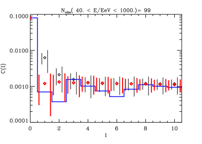
Figure 1: Angular power spectrum $C(l)$ as a function of multi-pole $l$, obtained for the AGASA+SUGAR exposure function, for $N_{\rm obs}=99$ events observed above 40 EeV. We show the realization averages (diamonds), statistical (left) and total (right) error bars, respectively, predicted by the model. The red (thick) diamonds and red (thick, outer) error bars represent scenario 6, whereas the black (thin) diamonds and black (thin, inner) error bars represent scenario 1. The histogram corresponds to the AGASA+SUGAR data.

It was noted in Ref. anchor_iso that the AGASA and SUGAR experiments had comparable exposure in the northern and southern hemisphere, respectively. Above $4\times 10^{19}\,$eV they combined 50 events observed by AGASA (excluding 7 events observed by Akeno) and 49 events seen by SUGAR. While SUGAR’s angular resolution is much worse than for AGASA and in general prevents a combination of the two data sets, multi-poles $l\leq 10$ are not sensitive to scales $\lesssim 10^{\circ}$. To take advantage of more statistics and more complete sky coverage, we therefore use the combined AGASA+SUGAR data set of 99 events above $4\times 10^{19}\,$eV when computing multi-poles $l\leq 10$. The results for scenarios 1 and 6 in Tab. 1 are compared in Fig. 1. In contrast, since the auto-correlation function and clustering are sensitive to small scales, when comparing with data above $4\times 10^{19}\,$eV we will only use the reported 57 AGASA+Akeno events.

No signs of anisotropy were found by either the AGASA or the SUGAR experiment down to $10^{19}\,$eV. We therefore also compute predictions for the multi-poles for $\simeq 1500$ events observed above $10^{19}\,$eV, using the combined exposure of AGASA+SUGAR. This is compared with an isotropic distribution in Fig. 2 for scenarios 1 and 6. The likelihoods for consistency with isotropy are also summarized in Tab. 1.

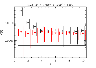
Figure 2: As Fig. 1, but for the angular power spectrum obtained for the combined AGASA+SUGAR exposure function, for $N_{\rm obs}=1500$ events observed above 10 EeV. The straight line is the analytical prediction, $C_{l}\simeq(4\pi N)^{-1}$, for the average multi-poles for complete isotropy.

Comparison in Tab. 1 of multi-poles, auto-correlation function and clustering above $4\times 10^{19}\,$eV, as well as observed isotropy at $10^{19}\,$eV, see Fig. 2, favor an observer immersed in relatively weak fields, especially scenario 6. For the multi-poles describing the large scale distribution this can qualitatively be understood as follows: Relatively strong fields surrounding the observer suppress the flux from the far sources. The observed flux is therefore more strongly dominated by the nearest few sources and thus more anisotropic. For observers immersed in weak fields, a relatively strong GZK cutoff is expected, inconsistent with AGASA data, see Fig. 3, and in contrast to the disfavored strong field observer.

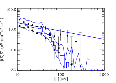
Figure 3: Predicted spectrum observable by AGASA for scenario 6, for which multi-poles were shown in Fig. 1, as compared to the AGASA (dots) and HiRes-I hires (stars) data. The histogram marks the average and the two lines above and below the 1-sigma fluctuations over the simulated realizations. The solid straight line marks the injection spectrum.

Scenarios 3 and 4 are somewhat disfavored by auto-correlation and clustering: Structured sources produce more clustering in the absence of magnetic fields. While this effect is only marginal in the current data set, it will provide a solid criterion for discriminating between the two scenarios in future experiments: Fig. 4 shows that the auto-correlation function is sensitive to the magnetic fields around the sources. Scenarios with no significant magnetic fields predict a stronger auto-correlation at small angles, independent of whether or not the sources are structured. This is because the images of sources immersed in considerable magnetic fields are smeared out, which also smears out the auto-correlation function over a few degrees. As shown in Fig. 4, this effect will become quite significant once $\sim 1500$ events are observed above $4\times 10^{19}\,$eV, for example, by the Pierre Auger project auger . It also appears robust against variation of other parameters such as source density and distribution: For example, whereas $N(1^{\circ})\simeq 10.1\pm 1.6$ for scenario 6, all other scenarios without magnetic field predict $N(1^{\circ})\gtrsim 16\pm 3$. Finally, all scenarios considered predict significant anisotropy above $4\times 10^{19}\,$eV for exposures reached by the Pierre Auger project.

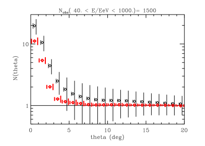
Figure 4: The auto-correlation function $N(\theta)$ as a function of angular distance $\theta$ for $N_{\rm obs}=1500$ events observed above 40 EeV in $1^{\circ}$ bins. The key for the model predictions is as in Figs. 1 and 3, now comparing scenario 6 (lower set) and 4 (upper set) instead, which only differ in the EGMF. $N(\theta)=1$ corresponds to isotropy.

Conclusions: Our results in Ref. sme showed that, in the case of structured extragalactic magnetic fields, the data were marginally consistent with an observer immersed in $\sim 0.1\,\mu$G field, although the isotropy of UHECRs at $10^{19}\,$eV could not be explained by a local source distribution alone. In the present paper we took into account sources up to cosmological distances and adopted more realistic distributions for the emission properties of UHECR sources. This considerably improved the quality of our fits at all energies. We conclude that the combination of statistical quantities characterizing the comparison between observed and simulated data moderately favors a scenario in which (i) UHECR sources have a density $n_{s}\sim 10^{-5}\,{\rm Mpc}^{-3}$ and follow the matter distribution (ii) magnetic fields are relatively pervasive within the large scale structure, including filaments, and with a strength of order of a $\mu$G in galaxy clusters (iii) the local extragalactic environment is characterized by a weak magnetic field below $0.1\,\mu$G. Thus, current UHECR data already allow us to probe the large scale distribution of matter and magnetic fields and seem to marginally confirm the quite realistic paradigm summarized above! This will increasingly be true for future detectors such as the Pierre Auger auger and EUSO euso projects. In particular, the degree-scale auto-correlation functions above $\simeq 4\times 10^{19}\,$eV can serve as a discriminator between magnetized and unmagnetized sources: $N(1^{\circ})\lesssim 10$ points to strong magnetization, rather independently of other source parameters. The best fit scenario also predicts a pronounced GZK cutoff.

FM acknowledges support by the Research and Training Network “The Physics of the Intergalactic Medium” under EU contract HPRN-CT2000-00126 RG29185. GS thanks the Max-Planck-Institut für Physik for hospitality and financial support.

References

- (1) P. Bhattacharjee and G. Sigl, Phys. Rept. 327 (2000) 109; L. Anchordoqui, T. Paul, S. Reucroft, and J. Swain, Int. J. Mod. Phys. A18 (2003) 2229.
- (2) K. Greisen, Phys. Rev. Lett. 16 (1966) 748; G. T. Zatsepin and V. A. Kuzmin, Pis’ma Zh. Eksp. Teor. Fiz. 4 (1966) 114 [JETP. Lett. 4 (1966) 78].
- (3) G. Sigl, M. Lemoine, and P. Biermann, Astropart. Phys. 10 (1999) 141; M. Lemoine, G. Sigl, and P. Biermann, e-print astro-ph/9903124; C. Isola, M. Lemoine, and G. Sigl, Phys. Rev. D 65 (2002) 023004; C. Isola and G. Sigl, Phys. Rev. D 66 (2002) 083002.
- (4) T. Stanev et al., Phys. Rev. D 62 (2000) 093005.
- (5) H. Yoshiguchi, S. Nagataki, S. Tsubaki, and K. Sato, Astrophys. J. 586 (2003) 1211; H. Yoshiguchi, S. Nagataki, and K. Sato, Astrophys. J. 592 (2003) 311; astro-ph/0307038.
- (6) G. Medina Tanco, Lect. Notes Phys. 576 (2001) 155.
- (7) G. Sigl, F. Miniati, and T. Enßlin, Phys. Rev. D 68 (2003) 043002.
- (8) R. M. Kulsrud, R. Cen, J. P. Ostriker, and D. Ryu, Astrophys. J., 480 (1997) 481
- (9) for a recent review see, e.g., J.-L. Han and R. Wielebinski, CHJA&A 2 (2002) 293 [e-print astro-ph/0209090].
- (10) F. Miniati, Mon. Not. R. Astron. Soc. 337 (2002) 199.
- (11) J. Chiang and R. Mukherjee, Astrophys. J. 496 (1998) 752.
- (12) M. Takeda et al., Phys. Rev. Lett. 81 (1998) 1163; Astrophys. J. 522 (1999) 225; Hayashida et al., e-print astro-ph/0008102; see also http ://www-akeno.icrr.u-tokyo.ac.jp/AGASA/.
- (13) M. M. Winn et al., J. Phys. G 12 (1986) 653; see also http://www.physics.usyd.edu.au/hienergy/sugar.html.
- (14) P. Sommers, Astropart. Phys. 14 (2001) 271.
- (15) L. Anchordoqui et al., e-print astro-ph/0305158.
- (16) G. Sigl, F. Miniati, and T. Enßlin, in preparation.
- (17) T. Abu-Zayyad et al. (HiRes collaboration), e-print astro-ph/0208243; e-print astro-ph/0208301.
- (18) J. W. Cronin, Nucl. Phys. B (Proc. Suppl.) 28B (1992) 213; The Pierre Auger Observatory Design Report (ed. 2), March 1997; see also http://www.auger.org.
- (19) See http://www.euso-mission.org.