Mass motions and chromospheres of RGB stars in the globular cluster NGC 2808

We present the results of the first observations, taken with FLAMES during Science Verification, of red giant branch (RGB) stars in the globular cluster NGC 2808. A total of 137 stars was observed, of which 20 at high resolution (R=47,000) with UVES and the others at lower resolution (R=19,000-29,000) with GIRAFFE in MEDUSA mode, monitoring $\sim$ 3 mag down from the RGB tip. Spectra were taken of the H$\alpha$, Na i D and Ca ii H and K lines. This is by far the largest and most complete collection of such data in globular cluster giants, both for the number of stars observed within one cluster, and for monitoring all the most important optical diagnostics of chromospheric activity/mass motions. Evidence of mass motions in the atmospheres was searched from asymmetry in the profiles and coreshifts of the H$\alpha$, Na i D and Ca ii K lines, as well as from H$\alpha$ emission wings. We have set the detection thresholds for the onset of H$\alpha$ emission, negative Na $D_{2}$ coreshifts and negative $K_{3}$ coreshifts at $\log L/L_{\odot}\sim$2.5, 2.9 and 2.8, respectively. These limits are significantly fainter than the results found by nearly all previous studies. Also the fraction of stars where these features have been detected has been increased significantly with respect to the previous studies. Our observations confirm the widespread presence of chromospheres among globular cluster giants, as it was found among Population I red giants. Some of the above diagnostics suggest clearly the presence of outward mass motions in the atmosphere of several stars.

1 Introduction

One of the most solid requirements of the stellar evolution theory is that some amount of mass loss (a few tenths of a solar mass) must occur during the evolutionary phases preceding the Horizontal Branch (HB) phase, in order to account for the observed HB morphologies in globular clusters (GC) (Castellani & Renzini 1968; Iben & Rood 1970; Rood 1973; Fusi Pecci & Renzini 1975, 1976; Renzini 1977). Also the pulsational properties of the RR Lyrae variables and the absence of asymptotic giant branch (AGB) stars brighter than the red giant branch (RGB) tip require that some mass has been lost during previous evolutionary phases (Christy 1966; Fusi Pecci et al. 1993; D’Cruz et al. 1996). Theoretical estimates of mass loss rates at the tip of the RGB are a few times $10^{-8}$ M_⊙ yr^-1 (Fusi Pecci & Renzini 1975, 1976; Renzini 1977). This would produce a few tens of solar masses of intracluster matter that should accumulate in the central regions of the clusters, in absence of sweeping mechanisms between Galactic plane crossings.

However, efforts to obtain direct evidence of intracluster matter, or of mass loss from individual RGB stars, have been only marginally successful. Diffuse gas in GC’s was detected only as an upper limit and well below 1 $M_{\odot}$ (Roberts 1988; Smith et al. 1990; Faulkner & Smith 1991; Freire et al. 2001), whereas the most recent search of mass loss evidence from individual RGB (or AGB) stars via ISOCAM IR-excess has indeed shown that dusty circumstellar envelopes are present in $\sim$ 15% of the giants in the $\sim$ 0.7 mag brightest interval (M${}_{\rm bol}\leq-2.5$) (Origlia et al. 2002, and references therein).

Spectroscopic surveys of a few hundred GC red giants (Cohen 1976, 1978, 1979, 1980, 1981; Mallia & Pagel 1978; Peterson 1981, 1982; Cacciari & Freeman 1983; Gratton et al. 1984) did reveal H$\alpha$ emission wings in a good fraction of stars brighter than log L/L${}_{\odot}\sim$ 2.7, i.e. along the upper 1.25 mag interval of the RGB. This was initially interpreted as evidence of an extended atmosphere, i.e. of mass loss. However, Dupree et al. (1984) demonstrated that this emission per se is not a unambiguous mass loss indicator, as it could arise naturally in a static stellar chromosphere, or it could be influenced by hydrodynamic processes due to pulsation (Dupree et al. 1994).

Profile asymmetry and coreshifts of chromospheric lines can reveal mass motions, and in particular the presence of a stellar wind and circumstellar material. Red giants in globular clusters were found to exhibit low velocity shifts in the cores of the H$\alpha$ or Na i D lines (cf. Peterson 1981; Bates et al. 1990, 1993); similarly, metal-poor field giants, which might be taken as the field counterparts of globular cluster giants, also indicate slow outflow from the asymmetries and line shifts in the H$\alpha$, Ca ii and Mg ii lines (Smith et al. 1992; Dupree & Smith 1995).

More recently, Lyons et al. (1996) discussed the Na i D and H$\alpha$ stellar profiles for a sample of 63 RGB stars in 5 GC (M4, M13, M22, M55 and $\omega$ Cen), and found evidence of significant Na i D core shifts in $\sim$ 50% of the stars brighter than $\log L/L_{\odot}\sim$2.9, whereas significant H$\alpha$ core shifts were detected in $\sim$ 50% of the stars brighter than $\log L/L_{\odot}\sim$2.5. These coreshifts are all $\leq$ 10 kms^-1, i.e. much smaller than the escape velocity from the stellar photosphere ($\sim$ 50-60 kms^-1).

Two RGB stars in NGC 6752 were studied by Dupree et al. (1994), by a detailed analysis of the Mg ii, Ca ii K and H$\alpha$ line profiles. These stars are at the RGB tip, and the Ca ii K and H$\alpha$ core shifts again revealed slow ($\leq$ 10 kms^-1) outflow motions. The asymmetries in the Mg ii lines, however, indicated under certain assumptions a stellar wind with a terminal velocity of $\sim$ 150 kms^-1, exceeding both the stellar photospheric escape velocity ($\sim$ 55 kms^-1) and the escape velocity from the cluster core ($\sim$ 23 kms^-1). The mass loss rate estimated by Dupree et al. (1994) from the Mg ii results ($\sim 10^{-9}$ M_⊙ yr^-1) would lead to a total mass loss of $\sim$ 0.2$M_{\odot}$ over the star lifetime on the RGB ($\sim 2\times 10^{8}$ yr), in very good agreement with the expectations of the stellar evolution theory. This result alone is not sufficient to meet the requirements of the stellar evolution that all stars suffer some degree of mass loss during the phases preceding the HB. However, it shows that the mass loss phenomenon along the RGB does indeed occur, even if perhaps only occasionally and detected among the brightest stars, and it may be revealed using visual indicators, although less effectively and accurately than using chromospheric lines in the UV such as the Mg ii, or in the near-IR such as the He i at 10830 Å (Dupree et al. 1992).

The advent of the multi-fibre spectrograph FLAMES on VLT2-Kueyen (Pasquini et al. 2002), with a multiplex capability of 8 with UVES (R=45000) and $\sim$ 130 with GIRAFFE in MEDUSA mode (R$\sim$15000–30000), allows a much more efficient monitoring of visual diagnostics of mass outflow along the RGB over a large magnitude range down from the RGB tip, especially in terms of sample size.

We have selected the globular cluster NGC 2808 for this monitoring, as it was the best candidate available for January-February observations, when Science Verification (SV) observations were scheduled.

Table 1: List of RGB stars observed with FLAMES during Science Verification on Jan 24 – Feb 02, 2003. Identification, coordinates and visual photometry are taken from Piotto et al. (2003), IR photometry is taken from the 2MASS Catalog.

ID n.	RA(2000)	DEC(2000)	B	V	J	H	K	Notes
7183	9 12 02.8710	-64 49 34.069	16.168	14.854				2
7536	9 12 31.7065	-64 49 22.268	15.812	14.372	11.802	11.069	10.829	1,2
7558	9 12 20.1287	-64 49 21.891	16.576	15.389	13.160	12.518	12.407	1
7788	9 11 57.1979	-64 49 14.551	16.168	14.870	12.472	11.777	11.623	1,2
8603	9 12 14.0510	-64 48 42.915	15.847	14.432	11.902	11.162	10.957	1
8679	9 11 44.5585	-64 48 39.890	16.164	14.961	12.753	12.156	12.022	1,2,F
8739	9 11 51.2018	-64 48 37.535	15.761	14.288	11.620	10.813	10.693	1,2
8826	9 12 09.8073	-64 48 33.243	16.275	15.033	12.746	12.057	11.911	1,2
9230	9 12 13.3528	-64 48 11.617	15.591	14.028	11.252	10.449	10.303	1
9724	9 12 00.9163	64 47 43.204	15.869	14.508	11.994	11.282	11.090	1,2
9992	9 12 46.8254	-64 47 23.732	15.402	13.702	10.729	9.886	9.659	2
10012	9 11 58.5661	-64 47 23.138	15.682	14.225	11.613	10.836	10.679	1,2
10105	9 12 21.1477	-64 47 13.906	15.976	14.669	12.279	11.564	11.417	1,2
10201	9 12 45.7573	-64 47 05.388	16.864	15.714	13.508	12.868	12.759	1,3
10265	9 11 56.6812	-64 47 00.535	15.728	14.309	11.772	11.026	10.823	1,2
10341	9 12 25.4161	-64 46 52.409	16.009	14.659	12.205	11.526	11.335	1,2
10571	9 12 41.1223	-64 46 25.848	15.806	14.376	11.771	10.988	10.844	1,2
10681	9 12 05.7235	-64 46 13.801	15.261	13.545	10.635	9.855	9.586	2
13575	9 11 31.6300	-64 49 02.281	16.615	15.386	13.090	12.417	12.270	1
13983	9 11 39.7915	-64 48 25.463	17.027	15.940	13.832	13.246	13.092	1,3
30523	9 11 22.4875	-64 55 23.351	16.658	15.489	13.320	12.697	12.550	1
30763	9 11 31.6195	-64 54 57.989	15.927	14.606	12.287	11.577	11.465	2
30900	9 11 36.3238	-64 54 47.078	16.319	15.084	12.890	12.203	12.075	1,2
30927	9 11 41.3502	-64 54 45.153	15.215	13.516	10.814	9.985	9.802	2
31851	9 11 14.3696	-64 53 36.046	16.420	15.221	13.064	12.411	12.280	1
32398	9 11 39.4612	-64 53 01.270	16.004	14.687	12.321	11.590	11.483	2
32469	9 11 16.3279	-64 52 55.955	15.485	14.040	11.531	10.777	10.689	1
32685	9 11 27.0742	-64 52 44.375	16.794	15.656	13.548	12.956	12.772	1,3
32862	9 11 42.0399	-64 52 34.140	16.379	15.166	12.871	12.171	11.999	1,2
32909	9 11 39.6760	-64 52 31.924	16.272	15.022	12.710	12.046	11.910	1
32924	9 11 22.2965	-64 52 31.081	16.138	14.853	12.515	11.785	11.701	1
33452	9 11 40.7982	-64 52 01.561	16.405	15.170	12.970	12.271	12.167	2
33918	9 11 01.6928	-64 51 36.087	15.776	14.331	11.756	11.021	10.887	1,2
34008	9 11 27.5242	-64 51 31.290	16.346	15.119	12.894	12.240	12.115	2
34013	9 11 23.8497	-64 51 30.965	17.499	16.444	14.503	13.897	13.843	3
35265	9 11 22.7197	-64 50 12.117	16.584	15.321	12.965	12.287	12.180	1
37496	9 12 13.8815	-64 57 09.411	16.126	14.871	12.586	11.891	11.730	1,2
37505	9 12 26.4217	-64 57 08.391	16.058	14.783	12.471	11.739	11.591	2
37781	9 12 13.0342	-64 56 41.142	16.148	15.037	13.001	12.396	12.307	1,F
37872	9 12 23.0712	-64 56 34.303	15.334	13.650	10.767	9.904	9.711	2,3
37998	9 12 12.5554	-64 56 24.603	15.638	14.233	11.706	10.960	10.796	1,2
38228	9 12 30.9696	-64 56 08.521	16.211	14.981	12.700	12.035	11.887	1
38244	9 12 08.9333	-64 56 07.955	16.378	15.193	12.996	12.307	12.177	1
38559	9 12 56.1453	-64 55 48.356	15.541	14.133	11.674	10.915	10.754	1,2,F
38660	9 12 39.8673	-64 55 43.083	15.772	14.452	11.995	11.407	9.519	2
38967	9 12 08.8682	-64 55 27.764	16.415	15.252	13.060	12.383	12.297	1
39060	9 12 14.5222	-64 55 24.085	15.793	14.417	11.939	11.193	11.036	1
39577	9 12 10.9820	-64 55 03.959	15.820	14.509	12.085	11.357	11.189	1,2,F
40196	9 12 05.9806	-64 54 43.265	15.894	14.570	12.142	11.440	11.264	2
40983	9 11 48.6726	-64 54 20.737	15.723	14.360	11.906	11.153	10.988	1,2
41008	9 12 17.6744	-64 54 19.865	16.339	15.189	12.973	12.309	12.200	1
41828	9 12 08.5555	-64 54 00.670	15.862	14.521	12.129	11.316	11.210	1
41969	9 11 50.8999	-64 53 57.615	15.787	14.446	11.972	11.254	11.092	1,2
42073	9 12 16.2176	-64 53 55.186	15.702	14.291	11.733	11.031	10.783	1

Table 1: (Continuation)

ID n.	RA(2000)	DEC(2000)	B	V	J	H	K	Notes
42165	9 12 33.7942	-64 53 52.922	17.430	16.387	14.369	13.816	13.613	1
42789	9 11 48.9406	-64 53 41.364	16.476	15.367	13.246	12.610	12.507	1
42886	9 12 59.1095	-64 53 38.608	17.019	15.921	13.780	13.157	13.040	1,3
42996	9 12 25.0560	-64 53 37.226	16.552	15.426	13.294	12.656	12.523	1
43041	9 12 40.0467	-64 53 35.930	15.349	13.723	10.869	10.063	9.822	1,2
43217	9 12 32.6714	-64 53 32.870	17.471	16.440	14.454	13.805	13.675	3
43247	9 12 10.1184	-64 53 32.654	16.022	14.786	12.486	11.732	11.543	1,2
43281	9 12 21.2449	-64 53 32.058	16.270	15.047				2
43333	9 12 55.0733	-64 53 30.392	16.570	15.473	13.408	12.776	12.698	1,F
43561	9 12 14.4769	-64 53 26.725	15.162	13.323	10.177	9.295	9.073	2
43794	9 12 26.3414	-64 53 22.607	15.861	14.554	12.157	11.468	11.271	1,2
43822	9 11 58.4947	-64 53 22.341	15.931	14.600	12.176	11.422	11.291	1,2
44573	9 12 06.1145	-64 53 08.983	16.285	15.089	12.709	12.022	11.912	2
44665	9 12 15.2786	-64 53 07.367	15.649	14.245	11.718	10.980	10.799	1,2
44716	9 12 17.8493	-64 53 06.449	16.123	14.899	12.605	11.924	11.748	2
44984	9 12 45.8780	-64 53 01.411	15.855	14.535	12.088	11.340	11.219	1,2
45162	9 11 59.2356	-64 52 59.262	15.172	13.263	10.019	9.074	8.853	2
45443	9 12 21.3723	-64 52 54.137	15.885	14.574	12.128	11.385	11.283	1,2
45840	9 12 11.1152	-64 52 47.477	15.552	14.117	11.516	10.703	10.536	1,2
46041	9 12 02.9671	-64 52 44.370	16.166	14.967	12.683	12.008	11.850	1,2
46099	9 12 33.5788	-64 52 43.088	15.375	13.741	10.915	10.044	9.835	2,3
46367	9 12 00.4581	-64 52 38.810	16.054	14.832	12.526	11.884	11.485	1
46422	9 11 56.0932	-64 52 37.896	15.174	13.376				3
46580	9 11 56.1904	-64 52 35.387	15.292	13.690				2,3
46663	9 12 17.0998	-64 52 33.946	15.860	14.551	12.146	11.456	11.323	1
46726	9 11 50.5738	-64 52 33.000	15.740	14.375	11.910	11.160	10.998	2
46868	9 12 09.7828	-64 52 30.452	16.003	14.752				1
46924	9 12 04.6008	-64 52 29.587	16.096	14.826				2
47031	9 12 00.9644	-64 52 27.851	15.605	14.181	11.593	10.894	10.355	2
47145	9 11 58.1949	-64 52 25.936	15.249	13.647	10.814	9.995	9.777	1,2
47421	9 11 56.4377	-64 52 21.270	15.571	14.175	11.674	10.834	10.696	1,2
47452	9 12 20.2257	-64 52 20.564	15.857	13.777	10.268	9.499	9.157	2
47606	9 12 06.6571	-64 52 18.225	15.257	13.436	10.227	9.349	9.103	2,3
48011	9 11 48.0108	-64 52 12.236	15.718	14.397	11.965	11.233	11.040	1,2
48060	9 11 55.1995	-64 52 11.458	15.256	13.556	10.609	9.741	9.523	1,2
48128	9 11 52.1753	-64 52 10.603	15.825	14.484	11.997	11.292	11.118	1,2
48424	9 12 06.6195	-64 52 05.871	15.772	14.452	11.995	11.407	9.519	2
48609	9 12 16.6443	-64 52 02.923	15.285	13.415	10.229	9.353	9.101	3
48889	9 12 08.5086	-64 51 58.467	15.139	13.341	10.340	9.431	9.253	2,3
49509	9 11 56.2108	-64 51 49.116	15.429	13.921	11.237	10.379	10.250	1
49680	9 12 10.0583	-64 51 46.474	15.256	13.567	10.573	9.706	9.497	1
49743	9 12 36.7974	-64 51 45.097	16.353	15.168	12.925	12.266	12.159	1,2
49753	9 12 06.8961	-64 51 45.474	15.669	14.350	11.804	11.018	10.886	2
49942	9 12 12.0864	-64 51 42.617	15.400	13.736	10.848	10.027	9.812	1
50119	9 11 42.9184	-64 51 39.752	15.425	13.886	11.210	10.382	10.218	2,3
50371	9 12 07.9720	-64 51 35.858	15.464	13.840	10.999	10.144	9.976	1
50561	9 12 23.1839	-64 51 32.695	16.120	14.834	12.428	11.725	11.548	2
50681	9 12 18.4772	-64 51 30.760	15.303	13.660	10.874	10.100	9.905	2
50761	9 11 57.0729	-64 51 29.676	15.394	13.390	9.947	9.096	8.827	2,3
50861	9 12 11.0865	-64 51 27.889	15.201	13.556	10.727	9.851	9.662	1,2
50866	9 11 54.2702	-64 51 27.928	15.941	14.634	12.219	11.524	11.353	1
50910	9 11 42.6346	-64 51 27.221	16.234	14.984	12.697	12.033	11.877	1
51416	9 12 29.2944	-64 51 18.935	16.188	14.945	12.619	11.911	11.803	1,2
51454	9 12 02.2715	-64 51 18.513	15.233	13.446	10.336	9.492	9.244	2,3
51499	9 12 07.3496	-64 51 17.800	15.157	13.435	10.447	9.567	9.382	2,3
51515	9 11 59.3832	-64 51 17.525	15.812	14.213	11.472	10.665	10.525	1,2
51646	9 11 50.3432	-64 51 15.395	16.550	15.460	13.425	12.791	12.668	1
51871	9 12 05.4500	-64 51 11.901	15.309	13.542	10.040	9.718	9.514	1

Table 1: (Continuation)

ID n.	RA(2000)	DEC(2000)	B	V	J	H	K	Notes
51930	9 11 49.9340	-64 51 10.872	15.531	14.068	11.422	10.655	10.478	2
51963	9 12 27.6355	-64 51 10.138	15.652	14.199	11.577	10.821	10.652	1,2
51983	9 12 02.5038	-64 51 10.068	15.328	13.474	10.294	9.391	9.182	3
52006	9 12 18.1017	-64 51 09.524	15.787	14.446	11.972	11.254	11.092	1,2
52048	9 12 05.7704	-64 51 80.996	15.645	14.259	10.387	11.012	10.797	2
52647	9 12 12.2817	-64 50 59.590	15.925	14.654	12.293	11.592	11.432	2
53284	9 12 01.4868	-64 50 49.350	15.501	13.847	10.902	9.254	9.953	2
53390	9 11 52.9455	-64 50 47.860	15.958	14.669	12.271	11.573	11.379	3
53579	9 11 48.7436	-64 50 44.801	15.830	14.461	11.877	11.178	10.992	2
54264	9 12 21.5127	-64 50 33.737	15.285	13.415	10.229	9.353	9.101	1
54284	9 11 54.7689	-64 50 33.662	15.789	14.407	11.877	11.148	10.985	1
54308	9 12 01.6780	-64 50 33.286	15.568	13.659	10.182	9.264	9.024	2
54733	9 12 07.8037	-64 50 26.397	15.602	14.128	11.523	10.761	10.571	1,2
54756	9 11 46.3335	-64 50 26.044	16.086	14.784	12.416	11.679	11.528	2
54789	9 12 00.4239	-64 50 25.567	15.626	14.247	11.756	11.019	10.863	1,2
55031	9 11 58.1972	-64 50 21.703	15.283	13.600	10.680	9.813	9.620	1
55354	9 12 10.3337	-64 50 16.108	16.024	14.749	12.406	11.655	11.531	2
55437	9 12 11.4613	-64 50 14.694	15.982	14.692	12.302	11.586	11.420	1
55609	9 12 29.9315	-64 50 11.384	16.078	14.751	12.301	11.575	11.467	1,2
55627	9 12 05.4152	-64 50 11.404	15.899	14.585	12.188	11.524	11.338	1
56032	9 11 45.5811	-64 50 04.209	15.579	13.976	11.112	10.292	10.095	3
56136	9 12 30.9806	-64 50 02.010	17.408	16.383	14.434	13.879	13.608	1
56536	9 12 04.3411	-64 49 55.639	15.301	13.626	10.785	9.896	9.688	2
56710	9 12 30.1594	-64 49 52.049	16.582	15.430	13.232	12.553	12.396	1
56924	9 12 15.1423	-64 49 48.859	15.629	14.207	11.587	10.869	10.676	2

Notes: 1=MEDUSA HR12 + HR14; 2=MEDUSA HR02; 3=UVES; F= field star.

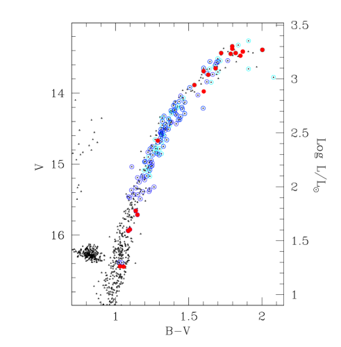
Figure 1: Colour-Magnitude diagram of NGC2808 (Piotto et al. 2003) showing the 137 RGB stars observed with FLAMES. Filled circles indicate the stars observed with UVES, open circles indicate the stars observed with GIRAFFE/MEDUSA.

Figure 2: Comparison of the temperatures and luminosities obtained using the Montegriffo et al. (1998, open circles) and Alonso et al. (1999,2001 filled dots) calibrations, for the $(B-V)$ colours (panel a) and $(V-K)$ colours (panel b).

Figure 3: Comparison of the temperatures obtained from the $(B-V)$ and $(V-K)$ colours, using Alonso et al. (1999,2001) calibration.

2 Observations and data reduction

The target selection and observation were made possible by the accurate UBV photometry and astrometry provided by Piotto et al. (2003). All stars have been checked to be free from companions closer than 2.4 arcsec and brighter than V+1.5, where V is the target magnitude. NGC 2808 is quite concentrated, and all target stars lie within a 7′ radius from the cluster centre, and this has put to a difficult test the capabilities of the FLAMES fiber positioner (FLAMES has a corrected field of view of 25′ diameter).

We show in Fig. 1 the Color-Magnitude diagram of NGC 2808: the tip of the RGB is at $V$ = 13.2, corresponding to M${}_{V}\sim$ –2.3, T${}_{\rm eff}\sim$3800 K, log L/L${}_{\odot}\sim$ 3.3, and M${}_{bol}\sim$ –3.5. We have selected 13 RGB stars within the uppermost 0.8 mag interval and 7 more sampling 2.5 fainter magnitudes, to be observed with UVES (R=47000, 8 single fibres of 1 arcsec entrance aperture, grating centred at 580nm and covering about 200nm). This wavelength range includes the Na i D and H$\alpha$ lines. The exposure times were 1800s for the stars with $V<14$ (except stars #50119, 51499 and 56032 that were observed for 3600s each), and $2\times 3600s$ for the stars with $V>14$ (except star #53390 that was observed for 3600s). Simultaneously, GIRAFFE in MEDUSA mode observed 117 more stars along the entire magnitude range with 3 setups, namely HR02 (Ca ii H+K, R=19600), HR12 (Na i D, R=18700) and HR14 (H$\alpha$, R=28800). The size of the MEDUSA fibres on the sky is 1.2 arcsec. The exposure times were $3\times 3600s$ with HR2, and 1800s each with HR12 and HR14. Not all the stars were observed with all the MEDUSA setups due to the high crowding conditions and the difficulty of placing the fibers; about one fourth were observed only with the HR02 or HR12+HR14 setups, but more than 50 have complete coperture of the interesting spectral features, either entirely with the GIRAFFE setups, or in combination with the UVES spectra. Table 1 gives in the last column information on the setups used for each star. We note that this is the first time that such a large sample of globular cluster RGB stars have been observed in all the major, deep optical lines (i.e., H$\alpha$, Na D and Ca ii H and K) that are normally used to study the presence of chromospheres and/or mass motions in the atmospheres.

Given the large interval in magnitude, S/N ratios vary a lot. In the case of the UVES spectra, S/N measured near 630 nm is about 100 for the brighter stars, and about 40 for the fainter ones, with 120 and 20 being the extremes. In the Ca ii region S/N’s were quite low (i.e. about 15 at the bottom of the K line for the brightest objects), while in the Na i D and H$\alpha$ setups they varied from about 25 to 150, following the luminosity distribution, with peaks around 80-100, and 50-60, respectively.

We collect the photometric information for our target stars in Table 1, including the IR photometry that is now available for all of our targets -except 6- in the 2MASS All-Sky Data Release (accessible at www.ipac.caltech.edu/2mass/releases/allsky/ and released on March 25, 2003).

The observations were performed during SV between January 24 and February 2, 2003. Most of the data were reduced by ESO personnel using the standard pipelines for FLAMES (see Pasquini et al. 2002 for a description), and were made public, according to ESO SV policies, on March 3, 2003. These reductions were intended to give a first insight on the data, and were not deemed optimal by the SV team: e.g., offsets in wavelegth calibrations between fibers could be present, in some cases producing errors of up to $\pm$ 10 kms^-1 in radial velocities (RV’s). We inspected our spectra and found them quite suitable for our purposes in two of the three GIRAFFE setups (HR02 and 12). The wavelength calibration for the H$\alpha$ setup HR14 was not quite so satisfactory, but no re-reduction of the HR14 spectra was performed since the GIRAFFE pipeline was still affected by a number of problems. However, for our purpose we mostly need to analyse H$\alpha$ profiles, and an accurate wavelength calibration over the entire wavelength range of HR14 is not essential, as long as it can be trusted over a small wavelength range encompassing H$\alpha$ itself and a few close photospheric lines. We then defined a pseudo-RV based on a few photospheric lines in the immediate vicinity of H$\alpha$, shifted to zero RV all the spectra, and retained for further analysis only the 50 Å centred on H$\alpha$. No attempt to derive centre/core shifts (see Sect. 4) was done on these spectra, but they are perfectly suitable to search for emissions. Because of these problems with wavelength calibration the subtraction of the sky contribution from the GIRAFFE spectra was not advisable. Direct contamination from sky lines could be excluded since the radial velocity of the cluster is $\sim$ 100 kms^-1. However, scattered sky light can in principle affect the line profiles, so we have estimated carefully the counts from the sky (using the dedicated fibres) and from the continuum and line core at H$\alpha$ for a few stars in the critical magnitude range V=14.0 to 15.0. For brighter stars the sky contamination becomes irrelevant, and for fainter stars no H$\alpha$ emission was detected (see Sect. 4.1.1). For homogeneity, we have treated the UVES spectra in the same way. We have thus estimated that neglecting the contribution of the sky scattered light can introduce an error of $\sim$2% with UVES at V=14, and of $\sim$1-2% with GIRAFFE at V=14.5-15.0. These are our thresholds for detecting H$\alpha$ emission, which appears to be much stronger than these values (see Sect. 4.1.1), therefore we are confident that neglecting the sky contribution in our analysis has not introduced any significant bias in our results.

As for the UVES spectra, we decided to reduce them again using the available UVES pipeline in order to obtain the best possible accuracy. FLAMES/UVES data require a rather careful treatment in order to remove both instrumental effects common to any high resolution, cross-dispersed echelle spectrograph and some specific ones due to its use in multi-object, fibre-fed mode. An ad-hoc Data Reduction Software (DRS) was specifically developed for this purpose, in the form of a set of procedures which are available as a context of the Münich Image Data Analysis System (MIDAS).

This DRS, described in detail elsewhere (Mulas et al. 2002), makes use of various flat-field exposures, taken both in fibre and in slit mode, to separately derive the pixel to pixel response of the detector and the contribution of each fibre to the overall distribution of light on the resulting two-dimensional science frame. The precise position of the orders and fibres is measured on the science frame itself. These pieces of information are then used together to perform an optimal extraction which, at the same time, carefully corrects for light contamination between fibres whose dispersed images are adjacent on the science frame.

Optimal extraction maximises the signal to noise ratio, since it does not discard the “wings” of the cross-dispersion point spread function (PSF) of the fibres, and effectively detects and removes most cosmic ray hits.

Exposures of a reference Th-Ar calibration lamp were extracted in exactly the same way as the science frames, to ensure the maximum coherence, and a 2-dimensional polynomial fit was performed on the detected lines to obtain the dispersion function of the spectrograph, separately for each fibre. The reference Th-Ar exposures were taken on the same day as the science data to be calibrated with them. The resulting wavelength calibration error resulted to be well below 0.01 Å throughout the wavelength range. Science spectra were rebinned to wavelength space and the echelle orders merged, making a weighted average where they overlap. Pixel by pixel variances were propagated by the DRS throughout the reduction procedure.

Both UVES and GIRAFFE spectra were then analysed using IRAF and ISA (Gratton 1988) to measure equivalent widths (EW’S) and RV’s. The RV’s were measured from the Doppler shifts of selected photospheric lines, mostly of Fe i, separately in the GIRAFFE setups (using rvidlines in IRAF on about 20 to 30 lines), and in the UVES spectra (using the ISA package). Errors are $\sim$ 0.6 kms^-1 for UVES and $\sim$ 1.5 kms^-1 for GIRAFFE. The observed RV’s were used to shift all spectra to zero radial velocity, thus eliminating any residual possible problem with the zero point shifts due to the non optimal calibration, which we found almost non existing anyway for the HR02 and 12 setups. Multiple exposures of the same star were coadded to enhance the S/N.

In a few cases the derived RV was strongly discrepant from the bulk of the other stars; this is a real effect, as confirmed by the spectral ranges where atmospheric or interstellar lines are present (e.g. the Na i D lines). We have assumed that those are field objects and have marked them with “F” in Table 1. They have not been included in the following analysis to avoid introducing spurious effects.

From the 20 stars observed with UVES we derive a mean heliocentric RV of 100.9 kms^-1 ($\sigma$ = 8.5), whereas from the lower precision GIRAFFE measures we obtain 102.1 kms^-1 ($\sigma$ = 10.9) using 81 member stars observed in the Na i region, and 99.0 kms^-1 ($\sigma$ = 10.3) using 83 stars observed in the Ca ii setup.

The first spectroscopic observations of NGC 2808 were taken by T.D. Kinman nearly 50 years ago: he set on a bright star in the center and exposed for about 3 hours, but because of guiding uncertainties the spectrum obtained was at least partially an integrated spectrum (Kinman 2003, private communication). The mean radial velocity derived from these data was 101$\pm$5 kms^-1 (Kinman 1959). Our results are in excellent agreement with this earliest determination. Later measures of mean radial velocity, summarised by Harris (1996, updated 2003) as 93.6$\pm$2.4 kms^-1, include values ranging from e.g. 80.1$\pm$9.9 (Rutledge et al. 1997), to 98$\pm$4 (Hesser et al. 1986), to 104.1$\pm$4.4 (Webbink 1981) kms^-1. The most discrepant result, by Rutledge et al. (1997), should probably be given little weight, as $\sim$25% of their results on globular clusters differ by more than 20 kms^-1 from the average of all previous determinations, and the authors say that the goal of their project was not to determine accurate cluster velocities.

Therefore all determinations, excluding Rutledge et al. (1997), are in agreement within 1-$\sigma$ error.

3 The physical and atmospheric parameters

Assuming for NGC 2808 the reddening E$(B-V)$ = 0.22 and apparent distance modulus $(m-M)_{V}$ = 15.59 (Harris 1996), we have calculated the intrinsic colours $(B-V)_{0}$ and $(V-K)_{0}$ and absolute magnitudes of our stars using the relations: E($V-K$) = 2.75 $\times$ E($B-V$), A_V = 3.1 $\times$ E($B-V$) and A_K = 0.35 $\times$ E($B-V$) (Cardelli et al. 1989).

The effective temperatures and bolometric corrections have been obtained both from visual and IR colours using two independent empirical calibrations specifically derived for late type giant stars by Montegriffo et al. (1998, their Table 3) and Alonso et al. (1999, their Eq.s #4, 9 and 17. See also Alonso et al. 2001). The metallicity assumed for NGC 2808 is [Fe/H]=–1.25 as an intermediate value among several determinations (cf. Walker 1999).

Transformations of the 2MASS K data to the ESO and TCS photometric systems, used by Montegriffo and Alonso respectively, have been performed using the relations provided by Carpenter (2001). The relations we have used are: $K_{ESO}=K_{2MASS}-0.005(J-K)_{2MASS}+0.045$ and $K_{TCS}=K_{2MASS}+0.006(J-K)_{2MASS}+0.002$. The relation for the TCS photometric system has been obtained via an intermediate passage through the CIT system.

The T_eff’s obtained from these two calibrations are compared in Fig. 2, where we see that they are quite compatible once allowance is made for a systematic offset that makes Alonso temperatures lower by $\simeq$ 153 ($\sigma$=65) and 88 ($\sigma$=17) K, when considering T_eff’s derived from $(B-V)$ and $(V-K)$ respectively.

This difference is irrelevant for the purpose of the present paper, where temperatures and luminosities are only used to locate correctly the stars in the HR diagram. It might be more relevant for a careful estimate of elemental abundances, but this aspect is discussed elsewhere (Carretta et al. 2003a,b). In the following we shall use Alonso et al. (1999, 2001) calibration as it is widely used and is therefore more convenient for comparison with other studies. With this calibration, the $(B-V)$ and $(V-K)$ colours yield similar results, except at the ends of the temperature range we are interested in, as we can see in Fig. 3; the average difference between the two T_eff’s is 19 ($\sigma$=95) K.

We list in Table 2 the values of temperature and luminosity we obtain for all our stars from the $(B-V)$ and $(V-K)$ colours and the Alonso et al. (1999, 2001) calibration, assuming $M_{{\rm bol},\odot}$ = 4.75. The values of gravity from the two colours are the same within 0.05 dex in the logarithm, and we list only the values derived from the $(B-V)$ colours.

Table 2: Physical and atmospheric parameters for our RGB stars in NGC2808. The last three columns give the measured heliocentric radial velocities for two GIRAFFE setups (HR02 and 12) and for UVES, derived by averaging several photospheric lines.

ID n.	MV	$(B-V)_{0}$	Teff	log L	log g	Teff	log L	RV02	RV12	RVU
			$(B-V)$	$(B-V)$	$(B-V)$	$(V-K)$	$(V-K)$	kms-1	kms-1	kms-1
7183	-0.736	1.094	4432	2.405	1.50			100.31
7536	-1.218	1.220	4261	2.645	1.19	4245	2.650	93.65	98.83
7558	-0.201	0.967	4618	2.150	1.83	4691	2.135		121.32
7788	-0.720	1.078	4454	2.394	1.52	4459	2.392	89.00	96.35
8603	-1.158	1.195	4294	2.612	1.24	4290	2.612		110.88
8739	-1.302	1.253	4219	2.692	1.13	4211	2.695	110.92	111.89
8826	-0.557	1.022	4536	2.310	1.64	4564	2.303	95.47	98.45
9230	-1.562	1.343	4107	2.836	0.94	4132	2.827		89.31
9724	-1.082	1.141	4366	2.561	1.32	4330	2.570	84.83	84.33
9992	-1.888	1.480	3949	3.041	0.67	3964	3.033	105.77
10012	-1.365	1.237	4239	2.711	1.12	4243	2.710	103.83	104.26
10105	-0.921	1.087	4442	2.477	1.44	4455	2.474	81.11	81.58
10201	0.124	0.930	4676	2.008	1.99	4717	2.000		111.21	105.96
10265	-1.281	1.199	4289	2.662	1.19	4283	2.664	106.50	108.70
10341	-0.931	1.130	4382	2.496	1.39	4399	2.492	99.97	102.53
10571	-1.214	1.210	4274	2.640	1.21	4252	2.646	106.20	112.98
10681	-2.045	1.496	3931	3.114	0.59	4005	3.074	97.07
13575	-0.204	1.009	4555	2.164	1.79	4569	2.161		95.33
13983	0.350	0.867	4777	1.899	2.14	4826	1.890		110.07	109.00
30523	-0.101	0.949	4646	2.104	1.89	4733	2.087		102.23
30763	-0.984	1.101	4422	2.507	1.40	4547	2.478	94.10
30900	-0.506	1.015	4546	2.287	1.67	4666	2.262	114.32	119.94
30927	-2.074	1.479	3950	3.115	0.59	4138	3.029	86.78
31851	-0.369	0.979	4600	2.220	1.75	4731	2.195		93.05
32398	-0.903	1.097	4427	2.473	1.43	4494	2.457	94.40
32469	-1.550	1.225	4255	2.780	1.06	4379	2.744		94.15
32685	0.066	0.918	4695	2.028	1.98	4788	2.010		87.17	94.52
32862	-0.424	0.993	4579	2.247	1.72	4525	2.258	98.57	105.16
32909	-0.568	1.030	4524	2.316	1.63	4572	2.306		90.43
32924	-0.737	1.065	4473	2.396	1.53	4538	2.381		101.03
33452	-0.420	1.015	4546	2.252	1.70	4671	2.226	92.79
33918	-1.259	1.225	4255	2.664	1.17	4312	2.647	117.58	119.80
34008	-0.471	1.007	4558	2.270	1.69	4670	2.247	102.73
34013	0.854	0.835	4830	1.688	2.37	5110	1.645			101.49
34634	-0.229	1.013	4549	2.175	1.78	4627	2.159
35265	-0.269	1.043	4505	2.201	1.74	4547	2.192		98.95
37496	-0.719	1.035	4516	2.378	1.56	4547	2.372	109.69	109.75
37505	-0.807	1.055	4487	2.420	1.51	4504	2.416	96.87
37872	-1.940	1.464	3967	3.052	0.66	4015	3.028	104.96		104.94
37998	-1.357	1.185	4307	2.687	1.17	4317	2.684	90.72	94.27
38228	-0.609	1.010	4553	2.326	1.63	4588	2.319		101.96
38244	-0.397	0.965	4621	2.227	1.75	4659	2.220		106.87
38660	-1.300	1.162	4338	2.656	1.22	4332	2.657	96.62
38967	-0.338	0.943	4655	2.197	1.80	4717	2.185		98.44
39060	-1.173	1.156	4346	2.602	1.27	4357	2.600		113.95
40196	-1.020	1.104	4418	2.522	1.38	4413	2.524	97.76
40983	-1.230	1.143	4364	2.620	1.26	4364	2.620	106.19	118.90
41008	-0.401	0.930	4676	2.218	1.78	4684	2.216		94.62
41828	-1.069	1.121	4394	2.548	1.35	4409	2.544		100.96
41969	-1.144	1.121	4394	2.578	1.32	4377	2.583	79.00	88.81
42073	-1.299	1.191	4299	2.666	1.19	4268	2.676		101.15
42165	0.797	0.823	4851	1.707	2.36	4906	1.698		108.81
42789	-0.223	0.889	4741	2.134	1.89	4813	2.122		115.68
42886	0.331	0.878	4759	1.910	2.12	4791	1.904		109.36	114.20
42996	-0.164	0.906	4714	2.116	1.90	4769	2.106		91.47
43041	-1.867	1.406	4033	2.990	0.75	4035	2.989	112.22	109.48

Table 2: (Continuation)

ID n.	MV	$(B-V)_{0}$	Teff	log L	log g	Teff	log L	RV02	RV12	RVU
			$(B-V)$	$(B-V)$	$(B-V)$	$(V-K)$	$(V-K)$	kms-1	kms-1	kms-1
43217	0.850	0.811	4871	1.683	2.39	4916	1.676			103.23
43247	-0.804	1.016	4544	2.406	1.55	4463	2.425	106.76	107.76
43281	-0.543	1.003	4564	2.298	1.66			95.23
43561	-2.267	1.619	3801	3.294	0.35	3872	3.240	92.69
43794	-1.036	1.087	4442	2.523	1.39	4431	2.526	97.95	101.91
43822	-0.990	1.111	4408	2.513	1.39	4411	2.512	88.92	99.96
44573	-0.501	0.976	4605	2.272	1.70	4516	2.291	88.63
44665	-1.345	1.184	4308	2.682	1.18	4310	2.681	91.94	93.67
44716	-0.691	1.004	4562	2.357	1.60	4539	2.362	99.30
44984	-1.055	1.100	4423	2.535	1.37	4405	2.540	86.65	82.96
45162	-2.327	1.689	3731	3.386	0.22	3810	3.310	112.90
45443	-1.016	1.091	4436	2.516	1.39	4425	2.519	99.23	96.10
45840	-1.473	1.215	4268	2.745	1.10	4220	2.760	95.49	100.90
46041	-0.623	0.979	4600	2.322	1.65	4568	2.329	93.63	103.22
46099	-1.849	1.414	4024	2.987	0.75	4032	2.983	102.55		103.48
46367	-0.758	1.002	4565	2.383	1.58	4383	2.427		95.19
46422	-2.214	1.578	3843	3.239	0.42					93.50
46580	-1.900	1.382	4061	2.991	0.77			102.34		103.12
46663	-1.039	1.089	4439	2.525	1.39	4474	2.516		97.26
46726	-1.215	1.145	4361	2.615	1.27	4360	2.616	90.03
46868	-0.838	1.031	4522	2.425	1.52				110.38
46924	-0.764	1.050	4495	2.402	1.53			96.36
47031	-1.409	1.204	4282	2.715	1.13	4076	2.788	95.43
47145	-1.943	1.382	4061	3.008	0.75	4051	3.012	66.67	75.97
47421	-1.415	1.176	4319	2.707	1.16	4288	2.716	74.65	69.43
47452	-1.813	1.860	3570	3.457	0.08	3737	3.174	101.28
47606	-2.154	1.601	3819	3.233	0.42	3839	3.218	96.25		97.77
48011	-1.193	1.101	4422	2.591	1.31	4375	2.603	98.87	101.85
48060	-2.034	1.480	3949	3.099	0.61	3969	3.088	96.03	91.58
48128	-1.106	1.121	4394	2.563	1.33	4368	2.570	96.16	101.22
48424	-1.138	1.100	4423	2.568	1.34	3649	3.020	109.01
48609	-2.175	1.650	3769	3.286	0.34	3846	3.221			85.20
48889	-2.249	1.578	3843	3.253	0.41	3943	3.188	114.00		116.29
49509	-1.669	1.288	4175	2.854	0.95	4164	2.858		106.58
49680	-2.023	1.469	3961	3.088	0.63	3952	3.094		83.64
49743	-0.422	0.965	4621	2.237	1.74	4665	2.228	107.18	112.48
49753	-1.240	1.099	4425	2.609	1.30	4298	2.643	112.04
49942	-1.854	1.444	3989	3.006	0.72	4023	2.990		118.85
50119	-1.704	1.319	4136	2.882	0.91	4166	2.871	100.83		101.56
50371	-1.750	1.404	4035	2.942	0.80	4054	2.934		104.36
50561	-0.756	1.066	4471	2.404	1.52	4429	2.414	92.71
50681	-1.930	1.423	4013	3.025	0.71	4114	2.981	115.24
50761	-2.200	1.784	3639	3.462	0.10	3756	3.309	103.34		99.80
50861	-2.034	1.425	4011	3.067	0.67	4039	3.054	108.07	110.60
50866	-0.956	1.087	4442	2.491	1.42	4432	2.493		95.50
50910	-0.606	1.030	4524	2.332	1.61	4577	2.320		98.33
51416	-0.645	1.023	4534	2.345	1.60	4546	2.342	87.40	90.40
51454	-2.144	1.567	3855	3.202	0.46	3893	3.177	82.79		83.35
51499	-2.155	1.502	3925	3.162	0.54	3960	3.142	108.71		109.18
51515	-1.377	1.379	4065	2.780	0.98	4154	2.745	104.52	106.77
51646	-0.130	0.870	4772	2.092	1.95	4886	2.072		99.69
51871	-2.048	1.547	3876	3.149	0.53	3970	3.094		93.84
51930	-1.522	1.243	4232	2.776	1.05	4214	2.782	90.34
51963	-1.391	1.233	4244	2.720	1.11	4242	2.720	100.59	102.54
51983	-2.116	1.634	3786	3.247	0.39	3855	3.191			101.48
52006	-1.268	1.111	4408	2.624	1.27	4397	2.627	108.92	109.48

Table 2: (Continuation)

ID n.	MV	$(B-V)_{0}$	Teff	log L	log g	Teff	log L	RV02	RV12	RVU
			$(B-V)$	$(B-V)$	$(B-V)$	$(V-K)$	$(V-K)$	kms-1	kms-1	kms-1
52048	-1.331	1.166	4333	2.670	1.20	4294	2.681	75.18
52647	-0.936	1.051	4493	2.471	1.46	4480	2.474	121.06
53284	-1.743	1.434	4001	2.956	0.77	4038	2.938	104.62
53390	-0.921	1.069	4467	2.471	1.45	4426	2.481			99.71
53579	-1.129	1.149	4356	2.582	1.30	4294	2.600	94.66
54264	-0.254	0.919	4693	2.156	1.85	4668	2.161		121.39
54284	-1.183	1.162	4338	2.609	1.26	4327	2.612		117.17
54308	-1.931	1.689	3731	3.228	0.38	3732	3.226	109.80
54733	-1.462	1.254	4217	2.757	1.07	4236	2.751	111.60	113.25
54756	-0.806	1.082	4449	2.429	1.49	4452	2.428	94.31
54789	-1.343	1.159	4342	2.672	1.20	4355	2.668	94.68	88.05
55031	-1.990	1.463	3968	3.072	0.64	3995	3.058		106.71
55354	-0.841	1.055	4487	2.434	1.50	4483	2.435	109.67
55437	-0.898	1.070	4466	2.462	1.46	4440	2.468		106.19
55609	-0.839	1.107	4413	2.451	1.45	4430	2.447	114.62	118.14
55627	-1.005	1.094	4432	2.513	1.40	4459	2.506		96.45
56032	-1.614	1.383	4060	2.877	0.88	4045	2.884			90.42
56136	0.793	0.805	4882	1.704	2.37	4905	1.700		115.11
56536	-1.964	1.455	3977	3.056	0.66	4016	3.037	107.17
56710	-0.160	0.932	4673	2.122	1.88	4643	2.128		115.35
56924	-1.383	1.202	4285	2.704	1.15	4252	2.714	98.65

4 Results and discussion

4.1 H$\alpha$ line

Figure 4: Normalised parts of spectra containing the H$\alpha$ line for the 20 stars observed with UVES, shifted to RV=0. We also plot the line bisectors for the brighter stars. Note that spectra for stars fainter than V=14.5 show the sky H$\alpha$ line in emission on the blue side of the stellar H$\alpha$ line.

4.1.1 Emission

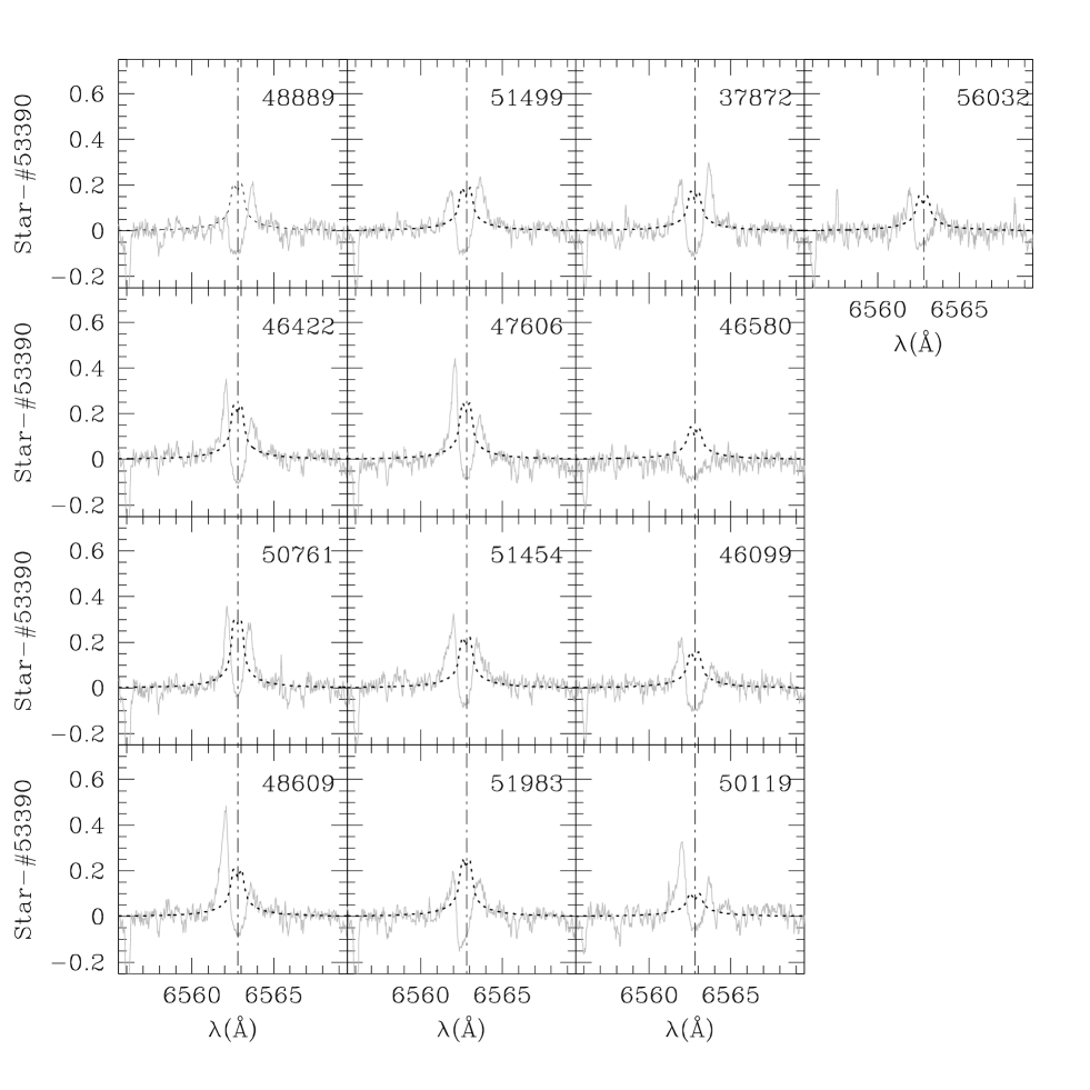
Figure 5: H$\alpha$ lines after subtraction of the template profile from star #53390, for the 13 stars observed with UVES and brighter than V=14.0 ($\log L/L_{\odot}$=2.88). The solid grey lines show the differences of the observed profiles, the dotted lines show the differences of the corresponding theoretical profiles.

We show in Fig. 4 the H$\alpha$ line profiles for the 20 stars observed with UVES. One can see that most of the stars brighter than V=14 show clear evidence of emission wings, mostly on the blue side, but also on both sides, whereas the fainter ones do not show such features. We note that weak emission from the wings could escape detection as it would be compensated by the absorption, the net result being a narrower absorption profile. In order to reveal all possible evidence of emission, after careful visual inspection we have arbitrarily identified a “template” star with no obvious H$\alpha$ emission and a fairly symmetric profile. This star is #53390 (V=14.67, $M_{V}$=–0.9, $T_{\rm eff}\sim 4400$K and $\log L/L_{\odot}\sim$2.5). We have then subtracted the H$\alpha$ profile of #53390 from all stars in our UVES sample brighter than V=14 after normalizing the intensities to the continuum and shifting in wavelength to superpose the bisector of the H$\alpha$ profile at the level of half maximum intensity. We have applied this procedure only to the stars in our UVES sample brighter than V=14.5 because the fainter ones become progressively hotter and the H$\alpha$ profiles have a different shape, besides showing no indication whatsoever of emission wings. However, the possible dependence of the H$\alpha$ line shape on temperature might introduce spurious features in the subtracted profiles. In order to test for this effect, we have calculated the theoretical H$\alpha$ profiles for our stars using Kurucz model atmospheres (with no chromosphere) and the individual values of temperature and gravity estimated from the (B–V) colors that are listed in Table 2. In Fig. 5 we show the difference of the observed spectra (star–#53390) and, for comparison, the difference of the corresponding theoretical profiles. Clearly the observed profiles are quite different from the theoretical ones as predicted just from the variations of temperature and gravity along the RGB. In particular: i) In all stars the absorption at the center of the line is larger than in the template star, contrarily to the theoretical expectations. This suggests the presence of a thicker atmosphere (i.e. an excess of material) and/or a higher temperature in the external regions (i.e. a chromosphere). This absorption is often blue-shifted, as it clearly appears in the stars 48889, 51499, 51454, 51983, 37872, 46580 and 56032. ii) Whereas the red emission wing could be due to the subtraction procedure in some case (see e.g. the stars 48609 or 56032), the blue emission wing seems real in all cases (except perhaps for star 51983). We note that the stars 48889 and 46580, that do not show blue emission, do however show an asymmetric blue-shifted absorption core like star 51983. From Fig. 5, therefore, it appears that 10 out of 11 stars brighter than $\log L/L_{\odot}\sim$2.9 (i.e. more than 90%) show H$\alpha$ emission wings. The faintest stars of this group, #50119 and 56032, have $\log L/L_{\odot}$=2.87-2.88; however we cannot take this value as a threshold for the onset of emission wings, since there is a gap of about half a magnitude in our UVES sample and the monitoring is not continuos in luminosity.

We have applied a similar procedure to the stars with $\log L/L_{\odot}>2.5$ that were observed with GIRAFFE/MEDUSA and setup HR14. Unlike for the UVES stars, we did not attempt to estimate the velocities of the emission peaks with respect to the bisector of the H$\alpha$ absorption profile, because of the shaky wavelength calibration. Instead, we have shifted spectra to RV=0 using nearby photospheric lines. In this case the template spectrum used for subtraction is the average of three spectra, i.e. those of stars #8603, 10571 and 43822, that have temperatures in the range $T_{\rm eff}$=4250-4400K and luminosities in the range $\log L/L_{\odot}$=2.50-2.65. These parameters are quite similar to those of star #53390 that was selected as a template for the UVES spectra. The much larger number of stars observed with GIRAFFE gives us a more detailed monitoring of the H$\alpha$ line behaviour as a function of luminosity, but of course the GIRAFFE lower resolution might more easily hide weak H$\alpha$ emission wings in the strong H$\alpha$ absorption line.

From the GIRAFFE sample we estimate that the fractions of stars showing some evidence of H$\alpha$ emission are approximately as indicated in parenthesis, in the luminosity intervals $\log L/L_{\odot}$=2.5-2.6 (30%), 2.6-2.7 (73%), 2.7-2.8 (86%), 2.8-2.9 (100%) and $>$2.9 (100%). If we include also the UVES results, in the interval $\log L/L_{\odot}>$2.9 the emission detection frequency would be $\sim$ 95%, and $\sim$ 94% for $\log L/L_{\odot}>$2.7.

A comparison with previous studies must take into account that the various sets of results were obtained with different procedures and with spectra of different resolution. Our procedure of subtracting an H$\alpha$ template, i.e. a supposedly pure absorption profile, was not chosen by anybody else before. In principle it should allow to detect emission features that might have gone unnoticed had this subtraction not been performed, therefore we would expect a higher detection rate because of this. On the other hand, we compare our UVES and GIRAFFE data, with spectral resolution of $\sim$7 and 10 km^-1 respectively, with the major statistical studies on H$\alpha$ emission in metal-poor red giant stars, namely Cacciari & Freeman (1983, 143 RGB stars in globular clusters, res. $\sim$30 kms^-1), Gratton et al. (1984, 113 RGB stars in globular clusters, res. $\sim$ 15 kms^-1), Smith & Dupree (1988, 52 metal-poor field red giants, res. $\sim$7 kms^-1), and Lyons et al. (1996, 62 RGB stars in globular clusters, res. $\sim$5 kms^-1). A poorer resolution makes the detection of emission features more difficult. As discussed also by Lyons et al. (1996), H$\alpha$ emission was detected by Cacciari & Freeman (1983) only among stars brighter than $\log L/L_{\odot}=$2.9 in a proportion of $\sim$33%, by Gratton et al. (1984) among stars brighter than $\log L/L_{\odot}=$2.7 in a proportion of $\sim$61%, by Smith & Dupree (1988) above the threshold of $M_{V}=-1.7$ (i.e. $\log L/L_{\odot}\sim 2.9$) in a proportion of $\sim$77% ($\leq$50% if reported to the threshold of $\log L/L_{\odot}=$2.7), and finally by Lyons et al. (1996) above the threshold of $\log L/L_{\odot}=$2.7 in a proportion of $\sim$ 80%.

Our detection limit for H$\alpha$ emission is $\log L/L_{\odot}\sim$2.9 from the UVES stars with a proportion of $\sim$91%; from the GIRAFFE stars our detection threshold is $\log L/L_{\odot}\sim$2.5 with a proportion of $\sim$72%. If we report these results to the threshold value of $\log L/L_{\odot}=$2.7 for the sake of comparison, and consider both UVES and GIRAFFE stars, then $\sim$94% of the stars brighter than this value exhibit H$\alpha$ emission wings.

Finally, we note that time variability of H$\alpha$ emission would contribute to underestimate the frequency of H$\alpha$ emitting stars. The present set of data, however, does not allow us to monitor for possible variability of H$\alpha$ emission features.

4.1.2 H$\alpha$ emission: mass loss or chromospheric activity?

The nature of the H$\alpha$ emission is controversial. Early studies (cf. Cohen 1976; Mallia & Pagel 1978; Cacciari & Freeman 1983; Gratton et al. 1984) assumed that it could be taken as evidence of extended matter around the star hence mass loss could be inferred. However, Dupree et al. (1984) argued that H$\alpha$ emission could form naturally in a static chromosphere, or it could be enhanced by hydrodynamic processes related to pulsation (Dupree et al. 1994), with no need to invoke mass loss (cf. also Reimers 1981). We discuss here briefly these two hypotheses.

In the hypothesis that the H$\alpha$ emission is due to circumstellar material, one could compare the observed EW of the emission components with “theoretical” predictions. These predictions are obtained by the use of two different relations, one by Cohen (1976) that gives the mass loss rate as:
$\dot{M}=2.4\times 10^{-11}V_{exp}R_{\ast}(R_{s}W_{\lambda})^{1/2}\times e^{(-1.1/T_{4})}\leavevmode\nobreak\ M_{\odot}yr^{-1}$
where it is assumed that the emission forms in a shell at constant expansion velocity $V_{exp}$ (taken as the observed velocity of the blue peaks listed in Table 3) and located at a distance ($R_{s}$) of 2 stellar radii ($R_{\ast}$) from the star, $W_{\lambda}$ is the equivalent width in Å  of the emission components, and $T_{4}$ is the brightness temperature of the star in units of 10⁴ K.
The other relation, by Reimers (1975), gives the mass loss rate as:
$\dot{M}=-4\times 10^{-13}\eta L/gR$
where all quantities are in solar units and $\eta$ is an empirical scaling factor that can reproduce reasonably well the HB morphology of globular clusters if allowed to vary in the range from 0.25 to 1.

By imposing that these two parameterizations yield the same value of mass loss rate, and using parameter values that can be derived from the observations or assumed under reasonable assumptions, one can then derive “theoretical” values for the EW’s of the emission components, to be compared with the observed ones. Fig. 6 shows a plot of the EW of the emission components, both for stars observed with UVES (starred symbols) and with GIRAFFE (open circles). A good fit of the estimated and observed EWs can be obtained for a value of $\eta\sim$0.5. This result does not mean that we are indeed observing mass loss via the H$\alpha$ emission wings, but only that this possibility is consistent with the admittedly very approximate and uncertain parameterizations available so far.

A difficulty with the Cohen circumstellar model, where the emission region is detached from the stellar atmosphere, is that it does not predict correctly the residual intensity at the center of the H$\alpha$ absorption. According to this model, in fact, the residual intensity should be larger (if some emission occurs at the stellar radial velocity), or at least equal to the undisturbed photospheric absorption. Therefore, we would expect that H$\alpha$ should be weaker in cooler stars and the residual intensity at the line center should increase with decreasing temperature. However, the opposite holds, as shown in Fig. 7. The strong absorption at the center of H$\alpha$ could be justified by assuming that the circumstellar material is disposed like a rotating torus around the star, but this explanation appears unjustified for single stars and it does not support mass loss.

The other hypothesis we are investigating is that the H$\alpha$ emission is due to chromospheric activity. The effects of a chromosphere on the profile of H$\alpha$ depend on the amount of material in the chromosphere itself. When the chromosphere is optically thin, the emission shows up at the center of the line, as it is the case for active (Population I) subgiants (Pasquini & Pallavicini 1991). In this case the emission causes a filling of the core of the line - its width is almost unaffected being essentially determined by thermal broadening. However, when the chromosphere is optically thick at the center of H$\alpha$ (this may occur if the lower level of the transition is populated by recombination from a strong enough UV flux in an extended and dense chromosphere), the line profile becomes very different. The mean free path of photons at the H$\alpha$ wavelength becomes short, and they cannot escape the atmosphere, unless they are slightly shifted in wavelength by anelastic diffusion processes: in this case, they will exit the atmosphere, causing blue- or red-shifted emissions. Detailed calculations of models with extended atmospheres by Dupree et al. (1984) indeed show deep central H$\alpha$ absorption with residual intensities $\leq$0.1, as well as blue- and red-shifted emissions. These predictions agree very well with our results for the coolest stars in our sample. We think this gives a strong support to the chromospheric explanation of the H$\alpha$ emission.

It should be reminded that the presence of an extended chromosphere neither excludes nor requires mass loss. This is shown by the wind model by Dupree et al. (1984), that describes a star with an extended chromosphere and a mass loss of $2\times 10^{-9}$ M$\odot\,yr^{-1}$. In the case of a net outflow motion, slightly red-shifted photons have a higher probability of escape, hence we expect that the red-shifted emission will be stronger than the blue-shifted one (see Fig. 3 of Dupree et al. 1984). We have estimated the relative strengths of the blue (B) and red (R) emission wings in our stars by integrating the flux distribution on the difference spectra in two 1Å-wide bands on the blue and red side of the absorption line (i.e. $\lambda\lambda$6561.3-6562.3 and 6563.3-6564.3), and further checked by visual inspection. The parameter B/R is reported in Tables 3 and 4 for the stars observed with UVES and GIRAFFE respectively, as $<$1 if the red emission wing is stronger (denoted as red asymmetry), $>$1 if the blue emission wing is stronger (blue asymmetry), and $\sim$1 if the red and blue wings are of similar strength: blue asymmetry appears to dominate. This confirms and reinforces the observational evidence found by Smith & Dupree (1988) among metal-deficient field red giants. Since all previous studies that could use repeated observations of the same stars found that both the emission-line strengths and the sense of the B/R asymmetry may change with time (on a timescale of months or even days) for any given star, no firm conclusions can be drawn from our data. We can only suggest the possible presence of differential mass motions in the line-forming region. Smith & Dupree (1988) proposed an alternative explanation of the variability of the emission strength (that we cannot detect but may indeed be present in our stars as well), i.e. fluctuations of the column density or the temperature gradient or both, within the chromosphere, possibly induced by pulsation.

In conclusion, as already noted by Dupree et al. (1984), asymmetries can be altered by episodic events, that may well occur in a (likely) variable chromosphere, as well as from a more complex geometry. Much more information should be obtained by examining the absorption profile, looking for evidence of core blue-shifts. These will be discussed in the next subsection.

Table 3: Parameters of the H$\alpha$ line for the stars observed with UVES. Columns 2-3 refer to the absorption core, columns 4-8 refer to the emission features. The parameter B/R is the intensity ratio of the Blue and Red emission wings after subtraction of the template spectrum.

ID n.	Centre	Core	B/R	Blue	Blue	Red	Red
	Sh.	Sh.		Pk.	Ter.	Pk.	Ter.
10201	-1.20	-0.76
13983	-0.31	0.60
32685	1.07	-0.76
34013	2.43	2.43
37872	-0.76	-2.57	$<$1	-44.3	-79.3	39.8	57.7
42886	0.60	0.60
43217	-0.31	1.99
46099	1.52	-1.20	$>$1	-42.3	-68.8	49.9	66.4
46422	1.52	-0.76	$>$1	-35.7	-77.5	41.1	79.2
46580	0.16	-2.57
47606	2.43	-0.31	$>$1	-34.6	-92.2	38.3	66.4
48609	1.99	-0.31	$>$1	-39.1	-86.7	38.7	65.5
48889	-0.76	-3.48	$<$1	-33.9	-42.4	39.6	61.8
50119	1.99	-0.76	$>$1	-39.6	-86.7	39.3	57.3
50761	0.60	-1.20	$\sim$1	-30.9	-67.0	31.9	52.8
51454	-1.20	-3.95	$>$1	-43.3	-83.0	35.3	75.5
51499	-1.65	-4.39	$<$1	-47.4	-85.7	39.3	79.2
51983	-1.20	-8.05	$\sim$1	-41.6	-83.0	35.2	55.9
53390	0.60	-0.76
56032	0.60	-4.39	$>$1	-38.5	-60.7	38.3	50.8

Notes:
i) All radial velocities (centre and core shifts, and velocities of emission peaks and terminal emission profiles) are given in kms^-1. Typical errors of individual measures are $\pm 1kms^{-1}$.
ii) The centre and core shifts are relative to the rest position of H$\alpha$, while the velocities of the emission peaks and terminal emission profiles are relative to the H$\alpha$ line centre (bisector at half maximum).

Table 4: Stars observed with GIRAFFE and showing H$\alpha$ emission. The parameter B/R indicates the relative strength of the H$\alpha$ blue and red emission wings after subtracting the template spectrum.

ID n.	B/R	Comments
7536	$\sim$1
8739	$\sim$1
9230	$>$1	Strong emission
9724	$>$1	Very weak
10265	$\sim$1
10341	$\sim$1
32469	$>$1
33918	$>$1
40983	$>$1
41969	$\sim$1
42073	$>$1
43041	$>$1
44665	$>$1
45840	$>$1
47145	$>$1
47421	$>$1
48011	$>$1
48060	$>$1
48128	$>$1
49509	$>$1
49680	$>$1	Strong emission
49942	$>$1
50371	$>$1
50861	$>$1	Strong emission
51515	$>$1
51871	$>$1	Strong emission
51963	$>$1	Very weak
52006	$\sim$1	Very weak
54284	$\sim$1	Weak
54733	$>$1	Weak
54789	$>$1
55031	$>$1	Strong emission

Figure 6: EWs of the emissions on the H$\alpha$ line wings, as a function of $M_{V}$. The lines show what is expected for different values of $\eta$.

Figure 7: Central residual intensity Rc of the H$\alpha$ line as a function of temperature, for the UVES stars only.

4.1.3 Shifts and line asymmetry

In the UVES spectra we derived the position of the H$\alpha$ absorption line by defining the center of the line as the bisector of the profile at half maximum intensity, and the core of the line as the minimum intensity interpolated by a local parabolic profile.

We have then measured the center and core shifts with respect to the nearby photospheric lines, and assumed that only shifts larger than 3$\sigma$ (i.e. $\sim$ 2 kms^-1) may be considered significant. Of the 20 stars observed with UVES, 8 show significant coreshifts, 7 of them being blueshifted (indicative of outward motion in the layer of the atmosphere where the H$\alpha$ line is formed) and 1 of them being redshifted (indicative of a downward flow). The blue-shifted ones are all brighter than $\log L/L_{\odot}\sim$2.88 and represent $\sim$54% of the UVES stars brighter than this value; the star with a red-shifted H$\alpha$ core is about 3 mag fainter. Only two stars show possibly significant centre shifts, both redward: one is the same star that shows also a redshifted core, the other one shows no significant coreshift. There is no apparent correlation between the occurrence of a blue coreshift and the asymmetry of the H$\alpha$ emission wings: of the 7 stars where a blue coreshift was detected, 2 have B/R$>$1, 3 have B/R$<$1, 1 has B/R$\sim$1 and 1 does not show emission wings. Five other stars exhibiting blue asymmetry do not show any significant coreshift. The GIRAFFE spectra have a resolution about a factor 2 worse than the UVES data, and the precision is hardly good enough to reveal coreshifts such as those detected in the UVES spectra, hence we did not try to estimate them.

Lyons et al. (1996), thanks to the higher resolution (R=60,000) of their spectra, were able to detect and measure significant H$\alpha$ coreshifts in $\sim$50% of stars brighter than $\log L/L_{\odot}\sim$2.5. We cannot reach this limit with our UVES data, and GIRAFFE’s resolution is not adequate for reliable measures of such small shifts. Therefore it appears that $\log L/L_{\odot}\sim$2.5 is the threshold for the occurrence of both H$\alpha$ emission (our present results) and H$\alpha$ coreshifts (Lyons et al. 1996), at least based on the presently available data.

In all cases the shifts are $\leq$10 kms^-1, as it was found also by Smith & Dupree (1988) from a sample of 52 metal-poor field red giants and using echelle spectra of similar resolution.

4.2 Na i D lines

Figure 8: The coreshifts of the Na i D₂ lines with respect to the photospheric LSR, as a function of the V magnitude. The filled circles indicate the stars observed with UVES, the open circles indicate the stars observed with GIRAFFE. Four stars have been observed by both, the two measures are connected by a line. Typical errors of the Na i D coreshifts are $\pm$ 0.6 kms^-1 for the UVES data and 1.5 kms^-1 for the GIRAFFE data, except for the faintest stars where the errors are larger.

In addition to the 20 stars that were observed with UVES, 82 more stars were observed with GIRAFFE/MEDUSA and setup HR12. The contributions from the interstellar Na lines are clearly separated, since the cluster heliocentric mean radial velocity is $\sim$ 100 kms^-1.

We have measured the coreshifts of both Na i D₁ and D₂ lines with respect to the photospheric LSR, and in Fig. 8 we show the shifts of the D₂ line (which are generally larger, i.e. more negative, than those of the D₁ line) as a function of magnitude for all our stars. As already commented by Lyons et al. (1996), “this suggests that, in most cases, there is an outward-increasing velocity gradient in the atmosphere of these cluster giants (although often for individual stars there is no significant velocity difference between the regions of the atmosphere where the Na D₂ and D₁ line cores are formed).” Typical errors of these measures are $\pm$ 0.6 kms^-1 for the UVES data and $\pm$ 1.5 kms^-1 for the GIRAFFE data, with slightly worse values for the faintest stars of our sample. We note that, within these errors, we do not detect any significant (i.e. $\geq 3\sigma$) coreshift in stars fainter than $M_{V}\sim-1.8$ (i.e. $\log L/L_{\odot}\geq$2.9). Considering only the UVES data, 8 out of the 11 stars brighter than this value show a significant negative coreshift, in very good agreement with the occurrence of the H$\alpha$ emission wings.

So, the luminosity limit of $\log L/L_{\odot}\sim$2.9 for the onset of significant Na D₂ coreshifts is the same as the value found by Lyons et al. (1996), but our detection frequency ($\sim$73%) is somewhat higher than theirs ($\sim$50%). Also, our values for the coreshifts of the D₂ line reach at most –4 kms^-1, whereas Lyons et al. (1996) found up to $\sim$ –8 kms^-1 in a few stars of the globular cluster M13 and one star in M55. This may be a real effect, or might be at least partly due to the resolution of our spectra that is a factor $\sim$1.3 lower than Lyons et al.’s.

Equivalent widths of the Na i D lines have been measured for all stars, and the D₂ line is the stronger of the Na i D pair, hence is formed higher in the atmosphere than the D₁ line (as also suggested by the larger velocities of the coreshifts). The values of the individual equivalent widths are not presented here, as they are used elsewhere (Carretta et al. 2003a,b) to perform a detailed Na abundance analysis.

Lyons et al. (1996) discuss in some detail the relationship between the coreshift and equivalent width of the Na D₂ line for their total sample of 63 stars in 5 globular clusters, and note that significant coreshifts are found only for stars with EW(D₂)$\geq$350 mÅ, with a frequency of about 45%. In all of their clusters the variation of the EW(D₂) is rather large, except in one cluster (M55) where all values of the EW(D₂) clump below 350 mÅ, and no significant coreshifts are detected. This strength threshold, however, does not seem to represent a physical threshold for the onset of mass-motion phenomena, since in the same M55 stars there is evidence for mass motions via H$\alpha$ coreshifts and/or asymmetric H$\alpha$ emission.

It is worth mentioning here that the strength of the D₂ line can vary significantly from star to star at any luminosity level due to intrinsic variations of the Na abundance, as it has been found in our NGC 2808 stars, as well as in other RGB stars previously studied in the globular clusters M13, M5, M15 and M92 (cf. Carretta et al. 2003a,b for a discussion). Based on Lyons et al. (1996) results, these variations in Na abundance within the same cluster RGB stars might lead to miss a significant fraction of D₂ coreshifts if the corresponding equivalent width happened to fall below the detection threshold of about 350 mÅ. Therefore, the use of the Na D₂ line negative coreshifts as indicators of mass motions in the atmospheres of red giants, as good as it may be, could underestimate the real frequency of this phenomenon because of this effect.

If chromospheric activity were at work, one might expect that the entire atmospheric structure is somewhat affected. The onset of H$\alpha$ emission seems to occur at $\log L/L_{\odot}\sim$2.5 and $T_{\rm eff}\sim$4400 K. It is interesting to note that, starting approximately at this value of temperature, the Na abundances derived by Carretta et al. (2003a,b) for hotter stars tend to be systematically lower, possibly suggesting some degree of line filling. Also the Fe abundances are slightly smaller, as if the region where these line form were hotter than predicted by the models.

4.3 Ca ii K lines

The Ca ii H and K lines are formed in the chromospheres of cool stars and appear as a deep absorption doublet with a central emission core that may be itself centrally reversed. These lines are often used to identify mass motions and the presence of circumstellar material in luminous stars via their asymmetries (see e.g. Reimers 1977a,b; Dupree 1986), but of course the presence of the chromosphere complicates their interpretation, as well as for the Na and H$\alpha$ lines, because of the similarity between the spectral signatures of chromospheres and mass loss.

We have observed 83 stars with the GIRAFFE HR02 setup centered on the Ca ii H and K lines: this is the first time that such a large collection of Ca ii H and K data for stars belonging to a globular cluster is available. Previous investigations of chromospheric activity in globular cluster giants using Ca ii K data were limited to two stars in NGC 6752 (Dupree et al. 1994). Our data show a well defined Ca ii reversal in several stars, and confirm the widespread presence of chromospheres among RGB stars of globular clusters.

We display in Fig. 9 the normalised region of the spectra containing the Ca ii H and K lines for some of the brightest stars we have observed. The insert shows the bottom of the K line for star #51499, zoomed to show the $K_{1}$, $K_{2}$ and $K_{3}$ components. If differential motions are present in the line-forming region, these peaks may be unequal in intensity and the central line core ($K_{3}$) shifted and asymmetric as the line opacity is moved to the blue (expansion) or to the red (contraction). Expansion causes the red emission peak ($K_{2r}$) to be strenghtened relative to the blue emission peak ($K_{2b}$), as clearly seen in Fig. 10.

Figure 9: Parts of spectra containing the Ca ii H and K lines, for some of the brightest stars we have observed. The insert shows the zoomed part of the K line for star #51499.

4.3.1 Emission frequency and asymmetries

We have observed 83 stars with the GIRAFFE/MEDUSA HR02 setup; of these, 22 show the central emission and reversal features described above. They are all brighter than V=14.4 ($\log L/L_{\odot}\sim$2.6), and represent approximately 50% of our observed sample in this upper luminosity interval.

For these stars we have measured the relative strength of the two peaks ($K_{2b}$ and $K_{2r}$) in the profile of the $K_{2}$ emission reversal, usually denoted by B/R (i.e. the ratio of the intensity of the short-wavelength to the long-wavelength peaks). The B and R intensities were estimated by fitting a Gaussian profile to both $K_{2b}$ and $K_{2r}$ components of the emission (see e.g. Dupree & Smith 1995). Only when the S/N was too poor, the relative intensities were estimated by eye. When outward motions are present in the line-forming region, the intensity ratio B/R$<$1 due to the increased opacity on the short-wavelength side of the line. In our sample, the onset of the B/R$<$1 (red) asymmetry seems to occur at $\log L/L_{\odot}\sim$2.87, and applies to about 75% of the stars brighter than this value.

We list in Table 5 these stars and corresponding B/R emission asymmetry.

Table 5: Parameters of the Ca ii K line. The $K_{3}$ shifts are measured relative to the nearby photospheric absorption lines.

Star ID.	B/R	logW	$K_{3}$ shift
		kms-1	kms-1
9992	$<$1	1.89	–6.71
10681	$<$1	2.00	–4.88
30927	$>$1:	1.98	–1.45
37872	$<$1	1.86	–5.03
43561	$>$1	1.97	–5.49
45162	$<$1:	1.99	–1.30
46099	$<$1	1.93	–8.47
46580	$<$1	1.89	–5.03
46726	$>$1	1.83	+3.36
47031	$>$1	1.80	–3.97
47606	$>$1:	1.93	–6.25
48889	$<$1	1.91	–5.19
50119	$<$1	1.87	–0.38
50681	$<$1	1.95	–6.10
50761	$>$1	2.06	–2.29
51454	$<$1	1.90	–7.70
51499	$<$1	1.99	–6.25
51930	$>$1	1.90	+12.89
52048	$>$1	1.87	+0.69
53284	$<$1	2.03	–12.20
56536	$<$1	1.90	+0.38
56924	$>$1:	1.83:	+6.41

4.3.2 Velocity shifts of the $K_{3}$ reversal

The $K_{3}$ self-reversal in the center of the $K_{2}$ emission line gives a direct measure of the velocity in the chromosphere at the highest point of Ca line formation. Velocities of the $K_{3}$ reversal have been measured relative to the nearby photospheric absorption lines. Typical uncertainties of these measures amount to $\pm$ 1.5 kms^-1, and we may assume again that only shifts larger than 3$\sigma$ (i.e. $\sim$ 4.5 km$s^{-1}$) can be considered significant. The values of the $K_{3}$ velocity shifts are listed in Table 5. They are more frequently negative than positive, mostly negative for the most luminous stars, and less than 15 kms^-1 for all stars listed in the table. This value is much less than is needed for escape from the photosphere, but mass loss cannot be excluded if a sufficiently high acceleration were attained at large distances from the star, depending on the acceleration mechanism.

Negative $K_{3}$ velocity shifts are taken to indicate that there is an outflow of material in the region of formation of the $K_{3}$ core reversal. We show in Fig. 10a a plot of the $K_{3}$ velocity shifts as a function of $M_{V}$ magnitude, where stars with red and blue $K_{2}$ emission asymmetries are indicated with different symbols: as expected, negative $K_{3}$ velocity shifts are more often associated with red asymmetries, reinforcing the indication of outward motions. These features are also found, to a much larger extent, in Population I bright giants where they suggest the presence of strong cool winds (cf. Dupree 1986). In Population II giants these winds, if present, would appear to be much weaker based on these diagnostics. In Fig. 10b we show the behaviour of the H$\alpha$ coreshifts relative to the $K_{3}$ velocity shifts for the 9 stars that have both sets of measures: 7 out of 9 stars define a clear tendency for more negative H$\alpha$ coreshifts to be associated with more negative $K_{3}$ coreshifts, stressing again the indication of outward motion; two stars (46099 and 47606) fall out of this trend, and this could be due to observational errors or variability in the H$\alpha$ profile, without pretending however to overinterpret the data.

Among our sample stars, the onset of negative $K_{3}$ coreshifts occurs at $\log L/L_{\odot}\sim$2.8, i. e. at a slightly lower luminosity than the onset of red asymmetry, and it applies to about 89% of the stars brighter than this value. This threshold is $\sim$0.2 mag fainter than the threshold estimated by Dupree & Smith (1995) and Smith & Dupree (1992) from metal-poor field red giants, who find significant negative $K_{3}$ shifts only among stars more luminous than $M_{V}$=–1.7 (i.e. $\log L/L_{\odot}\sim$2.88), in a proportion of $\sim$73%.

Figure 10: Panel a): $K_{3}$ velocity shifts as a function of luminosity. Stars with red asymmetry in the $K_{2}$ components (i.e. B/R$<$1) are shown as filled circles, stars with blue asymmetry (i.e. B/R$>$1) are indicated as open circles. Panel b): H$\alpha$ coreshift vs. $K_{3}$ velocity shifts for the 9 stars that have both sets of measures.

4.3.3 The Wilson-Bappu effect

The full width W of the emission reversal has been shown to be related to the absolute magnitude $M_{V}$ of a red giant stars (Wilson & Bappu 1957). The most recent calibration based on a sample of 119 nearby stars ($M_{V}$ derived from the Hipparcos database and W($K_{2}$) from high resolution spectra) has been provided by Pace et al. (2003), where an extensive discussion and references to the many previous studies are also given. The most recent analogous survey of metal-poor giants was presented by Dupree & Smith (1995), who analysed 24 metal-poor field red giants and found that, on average, they are more luminous than Population I giants at a given value of the Wilson-Bappu width W.

We have measured W for 22 of our stars following the same criteria described by Dupree & Smith (1995) and Pace et al. (2003), and we list the values of $\log$W in Table 4. We then show in Fig. 11 the values of $\log$W as a function of $M_{V}$, and compare them with the calibration for Population I stars given by Pace et al. (2003). In very close agreement with Dupree & Smith (1995) we also find that the luminosity distribution of our Population II giants is nearly flat and mostly contained within the interval $<M_{V}>\sim-1.9\pm 0.3$ mag, falling above the bright end of the $M_{V}$-$\log$W distribution for Population I giants.

In more detail, if we consider only the 17 stars brighter than V=14, they have $<V>$=13.55 and $\log<W>$=1.948: if we enter these values in the Pop.I relation we find $<M_{V}>$=–1.86 and (m–M)_V=15.41. These estimates compare very well with $<M_{V}>$=–2.04 based on the assumed distance modulus (m–M)_V=15.59, given the accuracy of this method on absolute magnitude (hence distance) determinations. This implies that, at least for these bright giants up to the metallicity of NGC 2808 ([Fe/H] $\sim$ –1.2), the dependence of the Wilson-Bappu law on metallicity seems smaller than estimated by Dupree & Smith (1995). Their statement “Use of the observed Ca ii K line width to derive an absolute magnitude with a calibration based on Population I stars will underestimate the true $<M_{V}>$ of a metal-deficient giant” is still true, but the error does not seem dramatic.

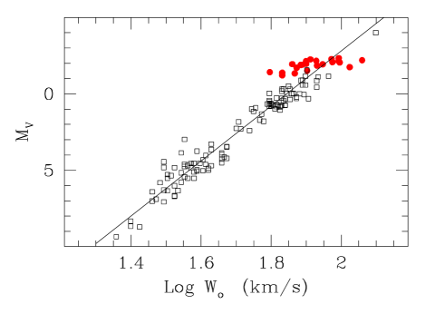
Figure 11: Wilson-Bappu effect: $\log$W as a function of $M_{V}$. The open squares show the Population I giants, and the filled circles show the NGC 2808 giants listed in Table 5. The line is the relation for Pop. I giants derived by Pace et al. (2003), $M_{V}=33.2-18\log W$ (r.m.s. error of the fitting is 0.6 mag).

5 Summary and Conclusions

We have observed a total of 137 RGB stars in the globular cluster NGC 2808 with the multi-fibre spectrograph FLAMES, and have measured the Ca ii K, Na i D and H$\alpha$ lines for 83, 98 and 98 stars respectively. We have searched for evidence of mass motions in the atmospheres using diagnostics such as absorption line coreshifts and asymmetries in emission components. This is the first time that such a large sample of globular cluster RGB stars have been observed in all the major optical lines that are normally used to study the presence of chromospheres and/or mass motions in the atmospheres.

Four of these stars are not cluster members, as their radial velocities differ by more than 3$\sigma$ from the cluster average velocity; for another star the metal abundance is abnormally large, suggesting either that the star is non-member or that it is an AGB star (hence the physical parameters used to calculate the metal abundance are incorrect).

From the remaining sample, we have obtained the following results:

• After subtracting a supposedly pure H$\alpha$ absorption template profile, we detect evidence of H$\alpha$ emission down to $\log L/L_{\odot}\sim$2.5 for $\sim$72% of stars; this proportion increases with luminosity and becomes $\sim$94% ($\sim$95%) among stars brighter than $\log L/L_{\odot}=$2.7 (2.9). Compared to all previous studies, including those based on higher spectral resolution such as Lyons et al. (1996), we have set the detection threshold for H$\alpha$ emission to a fainter limit and increased the fraction of stars where emission could be detected.
  The nature of this emission is not assessed definitely yet: our data favour a chromospheric rather than a circumstellar origin, however H$\alpha$ emission may be present in either stationary or moving chromospheres. Line coreshifts and asymmetries should in principle help distinguish between these two possibilities. For the coreshifts we have used only the 20 stars observed with UVES because of the better spectral resolution. We find that 7 out of these 20 stars, all brighter than $\log L/L_{\odot}\sim$2.88, show significant H$\alpha$ coreshifts. In all cases the shifts are less than 9 kms^-1, and negative (i.e. indicative of outward motion in the layer of the atmosphere where the H$\alpha$ line is formed).
  Asymmetry of the H$\alpha$ emission wings, indicated as the ratio B/R of the blue and red wing intensities, is mostly blue and does not seem to be correlated with the absorption coreshifts. However, its interpretation is likely complex as it is well known from previous studies that both the intensity of the emission wings and the sense of the asymmetry can be variable with time.

• Na D₁ and D₂ lines were observed for 20 stars with UVES and 82 stars with GIRAFFE. D₂ line coreshifts were measured for all of them, but significant negative values (i.e. $\geq 3\sigma$) were found only among UVES stars brighter than $\log L/L_{\odot}\sim$2.9, with a detection frequency of about 73%. This luminosity threshold for the onset of significant Na D₂ negative coreshifts is the same as the value found by Lyons et al. (1996), whose detection frequency is however of $\sim$50%. The values we find for the D₂ coreshifts reach at most –4 kms^-1, whereas Lyons et al. (1996) find values up to –8 kms^-1; this might be a real effect, or might be at least partly due to the lower resolution of our data.

  Equivalent widths of the Na i D lines have been derived for all stars, and used in separate papers (Carretta et al. 2003a,b) to perform a detailed abundance analysis. Because of possible intrinsic variations of Na abundance among RGB stars in a given cluster at any luminosity level, a significant fraction of negative D₂ line coreshifts might escape detection if the corresponding EW(D₂) is smaller than the detection threshold ($\sim$ 350 mÅ), according to Lyons et al. (1996) results.

• We have observed with GIRAFFE the Ca ii K line for 83 stars, 22 of which show the central emission K₂ and reversal K₃ features. The detection threshold for these features is $\log L/L_{\odot}\sim$2.6, and involves about 50% of our observed sample in this upper luminosity interval.
  Asymmetry B/R (i.e. the intensity ratio of the K_2b and K_2r components) could be detected in about 75% of stars brighter than $\log L/L_{\odot}\sim$2.9, and is mostly red (B/R$<$1) indicating outward motion.
  Velocity shifts of the K₃ reversal relative to the photospheric LSR have been measured, and are mostly negative indicating that there is an outflow of material in the region of formation of the K₃ core reversal. The onset of negative K₃ coreshifts occurs at $\log L/L_{\odot}\sim$2.8, i.e. at a slightly lower luminosity level than the onset of red asymmetry, and it applies to nearly 90% of the stars brighter than this value. Compared to previous results on metal-poor field red giants by Dupree & Smith (1995) and Smith & Dupree (1992), we have moved the detection threshold of negative K₃ coreshifts about 0.2 mag fainter, and we have increased by more than 20% the fraction of stars that display such property.

• We have measured the full width W of the Ca ii $K_{2}$ emission reversal in the same 22 stars discussed above, and compared them with the Wilson-Bappu relation, $\log$W as a function of $M_{V}$, defined by Pace et al. (2003) for Population I giants. We find that our Population II giants have a nearly constant luminosity $<M_{V}>\sim-1.9\pm 0.3$ mag, slightly brighter than the $M_{V}$-$\log$W distribution for Population I giants, confirming the results by Dupree & Smith (1995). Using the 17 brightest stars of our sample, we find that the dependence of the Wilson-Bappu law on metallicity is smaller than previously estimated.

In conclusion, our survey of RGB stars in NGC 2808 searching for mass motion diagnostics in their atmospheres has been able to reach fainter luminosity thresholds and monitor in much more detail along the RGB than any previous study in a given globular cluster. This is due to the FLAMES ability of reaching faint magnitudes with good S/N and good spectral resolution for a large number of stars simultaneously.

Although some of our diagnostics (e.g. H$\alpha$ emission) may not provide an unambiguous interpretation, other diagnostics give clear indications of the presence of both chromospheres and mass outflows in the atmospheres of these stars. However, we did not attempt to derive any estimate of mass loss rate, that depends on rather uncertain parameterizations of this phenomenon.

- (1) Alonso, A., Arribas, S. & Martinez-Roger, C. 1999, A&AS, 140, 261
- (2) Alonso, A., Arribas, S. & Martinez-Roger, C. 2001, A&A, 376, 1039 (Erratum)
- (3) Bates, B., Catney, M.G. & Keenan, F.P. 1990, MNRAS, 245, 238
- (4) Bates, B., Kemp, S.N. & Montgomery, A.S. 1993, A&AS, 97, 937
- (5) Cacciari, C. & Freeman, K.C. 1983, ApJ, 268, 185
- (6) Cardelli, J.A., Clayton, G.C. & Mathis, J.S. 1989, ApJ, 345, 245
- (7) Carpenter, J.M. 2001, AJ, 121, 2851
- (8) Carretta, E., Bragaglia, A., Cacciari, C. & Rossetti, E. 2003a, A&A, in press (astro-ph/0309021)
- (9) Carretta, E. et al. 2003b, in preparation
- (10) Castellani, V. & Renzini, A. 1968, Ap. Space Sci., 2, 310
- (11) Christy, R.F., 1966, ApJ, 144, 108
- (12) Cohen, J.G. 1976, ApJ, 203, L127
- (13) Cohen, J.G. 1978, ApJ, 223, 487
- (14) Cohen, J.G. 1979, ApJ, 231, 751
- (15) Cohen, J.G. 1980, ApJ, 241, 981
- (16) Cohen, J.G. 1981, ApJ, 247, 869
- (17) D’Cruz, N.L., Dorman, B., Rood, R.T. & O’Connell, R.W. 1996, ApJ, 466, 359
- (18) Dupree, A.K., Hartmann, L. & Avrett, E.H. 1984, ApJ, 281, L37
- (19) Dupree, A.K., Sasselov, D.D. & Lester, J.B. 1992, ApJ, 387, L85
- (20) Dupree, A.K., Hartmann, L., Smith, G.H., Rodgers, A.W., Roberts, W.H. & Zucker, D.B. 1994, ApJ, 421, 542
- (21) Dupree, A.K. & Smith, G.H. 1995, AJ, 110, 405
- (22) Faulkner, D.J & Smith, G.H. 1991, ApJ, 380, 441
- (23) Freire, P.C., Kramer, M., Lyne, A.G., Camilo, F., Manchester, R.N. & D’Amico, N. 2001, ApJ, 557, L105
- (24) Fusi Pecci, F. & Renzini, A. 1975, A&A, 39, 413
- (25) Fusi Pecci, F. & Renzini, A. 1976, A&A, 46, 447
- (26) Fusi Pecci, F., Ferraro, F.R., Bellazzini, M., Djorgovski, G.S., Piotto, G. & Buonanno, R. 1993, AJ, 105, 1145
- (27) Gratton, R.G., Pilachowski, C.A. & Sneden, C. 1984, A&A, 132, 11
- (28) Gratton R.G. 1988, Rome Obs. Preprint Ser. 29
- (29) Harris, W.E. 1996, AJ, 112, 1487 (2003 update in http://physun.physics.mcmaster.ca/Globular.html)
- (30) Hesser, J.E., Shawl, S.J., Meyer, J.E. 1986, PASP, 98, 403
- (31) Iben, I. & Rood, R.T. 1970, ApJ, 161, 587
- (32) Kinman, T.D. 1959, MNRAS, 119, 157
- (33) Lyons, M.A., Kemp, S.N., Bates, B. & Shaw, C.R. 1996, MNRAS, 280, 835
- (34) Mallia, E.A. & Pagel, B.E. 1978, MNRAS, 184, 55P
- (35) Montegriffo, P., Ferraro, F.R., Origlia, L. & Fusi Pecci, F. 1998, MNRAS, 297, 872
- (36) Mulas, G., Modigliani, A., Porceddu, I., & Damiani, F. 2002, Automatic data reduction in support of the FLAMES-UVES VLT Facility, 2002, Proceedings of SPIE Vol. 4844, 310
- (37) Origlia, L., Ferraro, F.R., Fusi Pecci, F. & Rood, R.T. 2002, ApJ, 571, 458
- (38) Pace, G., Pasquini, L. & Ortolani, S., 2003, A&A, 401, 997
- (39) Pasquini, L. & Pallavicini, R. 1991, A&A, 251, 199
- (40) Pasquini, L., Avila, G., Blecha, A. et al., 2002, The Messenger No. 110, p. 1
- (41) Peterson, R.C. 1981, ApJ, 248, L31
- (42) Peterson, R.C. 1982, ApJ, 258, 499
- (43) Piotto, G. et al. , 2003, in preparation
- (44) Reimers, D. 1975, Mem. Soc. R. Sci. Liège, 6th Ser. 8, 369
- (45) Reimers, D. 1977a, A&A57, 395
- (46) Reimers, D. 1977b, A&A61, 217
- (47) Renzini, A. 1977, in Advanced Stages of Stellar Evolution, eds P. Bouvier & A. Maeder, Saas-Fee (Geneva Observatory), p. 149
- (48) Roberts, M.S., 1988, in Globular Cluster Systems in Galaxies, eds J.E. Grindlay &A.G.D. Philip, (Dordrecht:Reidel), p. 411
- (49) Rood, R.T. 1973, ApJ, 184, 815
- (50) Rutledge, G.A., Hesser, J.E., Stetson, P.B., Mateo, M. Simard, L., Bolte, M., Friel, E.D., Copin, Y. 1997, PASP, 109, 883
- (51) Smith, G.H. & Dupree, A.K. 1988, AJ, 95, 1547
- (52) Smith, G.H., Wood, P.R., Faulkner, D.J. & Wright, A.E. 1990, ApJ, 353, 168
- (53) Smith, G.H., Dupree, A.K. & Churchill, C.W. 1992, AJ, 104, 2005
- (54) Walker, A.R. 1999, AJ, 118, 432
- (55) Webbink, R.F. 1981, ApJS, 45, 259
- (56) Wilson, O.C. & Bappu, M.K.V. 1957, ApJ, 125, 661