Incorporation of cosmic ray transport into the ZEUS MHD code

We present a numerical algorithm for the incorporation of the active cosmic ray transport, into the ZEUS-3D magnetohydrodynamical code. The cosmic ray transport is described by the diffusion-advection equation. The applied form of the diffusion tensor allows for anisotropic diffusion of cosmic rays along and across the magnetic field direction, which is controlled by two parameters: the parallel and perpendicular diffusion coefficients. The implemented numerical algorithm is tested by comparison of the diffusive transport of cosmic rays to analytical solutions of the diffusion equation. Our method is numerically stable for a wide range of diffusion coefficients, including the realistic values inferred from the observational data for the Milky Way of about $6\times 10^{28}{\rm\ cm}^{2}{\rm\ s}^{-1}$. The presented algorithm is applied for exemplary simulations of the the Parker instability triggered by cosmic rays injected by a single SN remnant.

1 Introduction

One of the major components of the interstellar medium (ISM), the cosmic ray (CR) gas, consists of relativistic electrons, protons and heavier atomic nuclei (see eg. Berezinski et al. 1990). It was shown beyond any doubt that the cosmic ray particles are accelerated in the process of diffusive acceleration by shocks associated with supernova remnants (SNR) in galactic disks (e.g. Koyama et al. 1995). Recent models suggest that the conversion rate of the supernova energy into cosmic ray energy is in the range of 10 - 50 % (see eg. Jones 1998 and references therein). The total kinetic energy output from a single supernova is of the order of $10^{51}{\rm\ erg}$, therefore the total CR energy per unit volume, produced within a supernova remnant, is significant as compared to thermal, kinetic and magnetic energy densities of the ISM.

Although the velocity of individual CR particles is close to the speed of light, the bulk motion of CR is diffusive and the CR bulk speed is of the order of Alfvén speed, i.e. typically a few tens of km/s. Recent studies by Giacalone and Jokipii (1999) and Jokipii (1999) suggest that the diffusion of cosmic ray gas in a turbulent magnetic field proceeds preferentially along the direction of the mean magnetic field. In our case the term cosmic rays means protons and nuclei but not electrons, since their contribution to the pressure is negligible. The estimations made by Strong and Moskalenko ( 1998) based on the GALPROP model provide the parallel diffusion coefficients of the order of $K_{\parallel}=6\times 10^{28}{\rm\ cm}^{2}{\rm\ s}^{-1}$. This value is 2-3 orders of magnitude larger than the diffusion coefficient for turbulent mixing of the ISM. The large energies carried by the cosmic ray component as well as its highly diffusive nature imply that the cosmic ray component cannot be neglected in the studies of dynamics of the ISM. That statement follows directly from investigations of stability of the ISM on spatial scales of the order of one up to a few kiloparsecs. Parker (1966, 1967) found that the multicomponent interstellar medium stratified by vertical gravity is subject to an instability which is caused by the buoyancy of the weightless ISM components, i.e magnetic field and cosmic rays.

The Parker instability has been extensively studied by numerous authors in the linear approximation under various circumstances like different disk gravity models (Giz & Shu 1993; Kim & Hong 1998), rigid and differential rotation (Shu 1974; Foglizzo & Tagger 1994, 1995; Hanasz & Lesch 1997) the presence of random magnetic field component (Parker & Jokipii 2000; Kim & Ryu 2001) and nonadiabatic effects in the ISM (Kosinski & Hanasz 2003).

Majority of the work was done within the limit of very large diffusion of cosmic rays along magnetic field lines and negligible diffusion across magnetic field lines. The effect of finite diffusion was studied by Kuznetsov and Ptuskin (1983) and recently by Ryu et al. (2003), who demonstrate that within the linear approximation incorporation of the diffusion-advection equation and realistic diffusion coefficients leads to results consistent with the mentioned simplified description of cosmic ray transport. According to the analysis done by Ryu et al. (2003) the finiteness of the diffusion coefficient decreases the growth rate of the Parker instability.

On the other hand numerical studies of the Parker instability investigate the effects of uniform vertical gravity (Kim et al. 1998), realistic vertical gravity (Kim et al. 2000), selfgravity (Chou et al. 2000), the effects of spiral arms (Franco et al. 2002), finite resistivity (Hanasz et al. 2002, Tanuma 2003; Kowal et al 2003), partial ionization (Birk 2002) and coupling to other disk instabilities (Kim, Ostriker & Stone 2002).

Surprisingly, the powerful cosmic ray component, which according to the linear analysis is crucial for the growth rate of the Parker instability, is neglected in numerical studies except the recent paper by Hanasz & Lesch (2000) who incorporate the diffusion-advection equation for the cosmic ray transport along magnetic field and study the Parker instability triggered by cosmic ray injection in SN remnants, applying the thin fluxtube approximation. That paper demonstrates the importance of the cosmic ray component for the global dynamics of the ISM, including the hydromagnetic dynamo effect.

In this paper we describe how to introduce the cosmic ray component, within the diffusion-advection equation, into the ZEUS-3D MHD code (Stone & Norman 1992a, 1992b) developped at the Laboratory of Computational Astrophysics (NCSA, University of Illinois at Urbana Champaign, see http://lca.ncsa.uiuc.edu/lca_codes_docs.html). The ZEUS code uses a time-explicit, operator-split, finite-difference method to solve the MHD equations on a staggered mesh. The MHD algorithm employs the constrained transport formalism and the method of characteristics for accurate propagation of Alfvén waves (Evans & Hawley 1988, Hawley & Stone 1995).

In the present paper we focus on the numerical method for the active cosmic-ray transport. In Section 2. we introduce the set of basic equations. The numerical algorithm is described in section 3, followed by tests of the numerical method and a comparison of some results of computations to analytical solutions in section 4. Section 5 contains as an example an application of the extended code for studies of the Parker instability triggered by the cosmic ray injection in a single SN remnant. Finally in Section 6. we summarize our results.

2 Equations of MHD including cosmic-ray transport

The diffusive cosmic ray (CR) transport on macroscopic astrophysical scales is described by the diffusion-advection equation. Following Schlickeiser and Lerche (1985) we apply the following form of the transport equation

$$\frac{{\partial}{e_{\rm cr}}}{{\partial}{t}}+\mbox{{\boldmath$\nabla$}}\left(e_{\rm cr}\mbox{{\boldmath$v$}}\right)=\mbox{{\boldmath$\nabla$}}\left(\hat{K}\mbox{{\boldmath$\nabla$}}e_{cr}\right)-p_{\rm cr}\left(\mbox{{\boldmath$\nabla$}}\cdot\mbox{{\boldmath$v$}}\right)+Q,$$ (1)

where $e_{\rm cr}$ and $p_{\rm cr}=(\gamma_{\rm cr}-1)e_{\rm cr}$ are the cosmic ray energy density and cosmic ray pressure, $\gamma_{\rm cr}$ (=4/3 in this paper) denotes the ratio of the specific heats of the relativistic cosmic ray gas, $\hat{K}$ presents the diffusion tensor, $v$ is velocity of the thermal gas and $Q$ is the source term for the CR energy density resulting from the cosmic ray injection by supernova remnants (SNR) or alternative sources. We note that eq. (1) assumes that cosmic rays are treated as a magnetized relativistic gas. This assumption holds as long as the particles are tied to the magnetic field, i.e. as long as they gyroradius is significantly smaller than the characteristic spatial scales of the magnetic field. Only cosmic rays with ultrahigh energies are ruled out by our approach since their gyroradius is larger than the thickness of the galactic disk. Eq. (1) implicitly assumes that the diffusion tensor describes the interaction of charged particles with magnetic fluctuations which appear on spatial scales considerably smaller than the characteristic scales in the interstellar medium. In the limit of low energies ($<100$ MeV) the the current approximation is not valid because cosmic-ray energy losses become important, although, the cosmic ray pressure still resides in that range.

In the present approach we apply the concept of anisotropic cosmic ray diffusion following Giaccalone and Jokipii (1999), Jokipii (1999), Hanasz and Lesch (2000) and Ryu et al (2003). In order to describe formally the anisotropic cosmic ray diffusion we implement the diffusion tensor (see e.g. Ryu et al. 2003) of the form

$$K_{ij}=K_{\rm\perp}\delta_{ij}+(K_{\parallel}-K_{\rm\perp})n_{i}n_{j},$$ (2)

where $n_{i}=B_{i}/B$ are components of the unit vectors tangent to magnetic field lines. The above cosmic-ray transport equation supplements the standard set of ideal MHD equations

$$\frac{{\partial}{\rho}}{{\partial}{t}}+\mbox{{\boldmath$\nabla$}}\cdot(\rho\mbox{{\boldmath$v$}})=0,$$ (3)

$$\frac{{\partial}{e}}{{\partial}{t}}+\mbox{{\boldmath$\nabla$}}\cdot\left(e\mbox{{\boldmath$v$}}\right)=-p\left(\mbox{{\boldmath$\nabla$}}\cdot\mbox{{\boldmath$v$}}\right),$$ (4)

$$\frac{{\partial}{\mbox{{\boldmath$v$}}}}{{\partial}{t}}+(\mbox{{\boldmath$v$}}\cdot\mbox{{\boldmath$\nabla$}})\mbox{{\boldmath$v$}}=-\frac{1}{\rho}\mbox{{\boldmath$\nabla$}}\left(p+p_{\rm cr}+\frac{B^{2}}{8\pi}\right)+\frac{\mbox{{\boldmath$B\cdot\nabla B$}}}{4\pi\rho},$$ (5)

$$\frac{{\partial}{\mbox{{\boldmath$B$}}}}{{\partial}{t}}=\mbox{{\boldmath$\nabla$}}\times\left(\mbox{{\boldmath$v$}}\times\mbox{{\boldmath$B$}}\right).$$ (6)

where the gradient of cosmic ray pressure $\mbox{{\boldmath$\nabla$}}p_{\rm cr}$ has been included in the equation of gas motion (see Berezinski et al. 1990). The other symbols have their usual meaning.

3 Numerical algorithm for the cosmic ray transport

The actual form of the diffusion-advection equation (1) is similar to the energy equation (4) except the diffusion term, therefore we incorporate an integration algorithm for the advection part of the cosmic-ray transport, following the method of integration of the energy equation (see Stone and Norman 1992a,b).

The integration method for the energy equation consists of a source step and a transport step. In the source step the $-p\mbox{{\boldmath$\nabla$}}\mbox{{\boldmath$v$}}$ term is evaluated together with possible explicit sources of the internal energy. In the transport step fluxes of internal energy, through cell boundaries, are computed using directional splitting. The total amount of internal energy within each cell is subsequently updated according to the sum of fluxes through all cell boundaries.

The implementation of the cosmic ray transport requires an additional contribution of diffusive fluxes

$$\mbox{{\boldmath$F$}}^{d}_{cr}=\hat{K}\mbox{{\boldmath$\nabla$}}e_{cr}$$ (7)

corresponding to the term $\mbox{{\boldmath$\nabla$}}\left(\hat{K}\mbox{{\boldmath$\nabla$}}e_{cr}\right)$ in the cosmic ray diffusion-advection equation. The tensorial form of the diffusion coefficient $\hat{K}$ is used to describe the anisotropic cosmic ray diffusion.

In order to incorporate the diffusion of cosmic rays in the numerical algorithm, along the magnetic field lines one should compute first components of the unit vector $\mbox{{\boldmath$n$}}=\mbox{{\boldmath$B$}}/B$ parallel to the magnetic field direction, separately for each cell face. Since in the ZEUS code vector field components are centered on different cell faces an averaging is necessary for these vector components which are parallel to the given cell face. For instance, the magnetic field components on 1-faces (assigned with the superscript ’1f’) are given by

$$\mbox{{\boldmath$B$}}^{\rm 1f}_{(i,j,k)}=[B_{1(i,j,k)},\makebox[156.49014pt]{}$$ (8)

$$0.25(B_{2(i,j,k)}+B_{2(i-1,j,k)}+B_{2(i-1,j+1,k)}+B_{2(i,j+1,k))},$$

$$0.25(B_{3(i,j,k)}+B_{3(i-1,j,k)}+B_{3(i-1,j,k+1)}+B_{3(i,j,k+1)})].$$

The field components on the other faces are computed analogously.

The next step is a computation of cosmic-ray diffusive fluxes across cell interfaces. This requires a prior computation of components of the gradient of cosmic-ray energy density. All three gradient components contributing to fluxes through a given cell-face should be centered at the center of that cell-face. Moreover, a monotinization of derivatives is essential for the numerical stability of the overall algorithm as soon as cosmic rays are coupled to the gas dynamics through the $\mbox{{\boldmath$\nabla$}}p_{\rm cr}$ term in the equation of gas motion. We apply the following formulae for numerical derivatives needed for the the flux components through the 1-faces:

$$(\nabla e_{\rm cr})_{(i,j,k)}^{\rm 1f}=[(d_{x}e_{{\rm cr}})_{(i,j,k)},(d_{y}e_{{\rm cr}})_{(i,j,k)},(d_{z}e_{{\rm cr}})_{(i,j,k)}],$$ (9)

where

$$(d_{x}e_{{\rm cr}})_{(i,j,k)}=(e_{{\rm cr}(i,j,k)}-e_{{\rm cr}(i-1,j,k)})/(x_{(i)}-x_{(i-1)}),$$ (10)

$$(d_{y}e_{{\rm cr}})_{(i,j,k)} = 0.25(d_{y,l}e_{{\rm cr}}+d_{y,r}e_{{\rm cr}})$$

$$\times(1+{\rm sign}(1,d_{y,l}e_{{\rm cr}}\ d_{y,r}e_{{\rm cr}})),$$

$$(d_{z}e_{{\rm cr}})_{(i,j,k)} = 0.25(d_{z,l}e_{{\rm cr}}+d_{z,r}e_{{\rm cr}})$$

$$\times(1+{\rm sign}(1,d_{z,l}e_{{\rm cr}}\ d_{z,r}e_{{\rm cr}})),$$

and the left and right derivatives used in the above formulae are given by

$$d_{y,l}e_{\rm cr} = 0.5((e_{{\rm cr}(i-1,j,k)}+e_{{\rm cr}(i,j,k)})$$

$$-(e_{{\rm cr}(i-1,j-1,k)}+e_{{\rm cr}(i,j-1,k)}))/(y_{(j)}-y_{(j-1)}),$$

$$d_{y,r}e_{\rm cr} = 0.5((e_{{\rm cr}(i-1,j+1,k)}+e_{{\rm cr}(i,j+1,k)})$$

$$-(e_{{\rm cr}(i-1,j,k)}+e_{{\rm cr}(i,j,k)}))/(y_{(j+1)}-y_{(j)}),$$

$$d_{z,l}e_{\rm cr} = 0.5((e_{{\rm cr}(i-1,j,k)}+e_{{\rm cr}(i,j,k)})$$

$$-(e_{{\rm cr}(i-1,j,k-1)}+e_{{\rm cr}(i,j,k-1)}))/(z_{(k)}-z_{(k-1)}),$$

$$d_{z,r}e_{\rm cr} = 0.5((e_{{\rm cr}(i-1,j,k+1)}+e_{{\rm cr}(i,j,k+1)})$$

$$-(e_{{\rm cr}(i-1,j,k)}+e_{{\rm cr}(i,j,k)}))/(z_{(k+1)}-z_{(k)}).$$

The monotonized derivatives used in formulae (3) and (3) reduce to centered derivatives if signs of left and right derivatives are the same. The cosmic ray energy fluxes through the cell-faces in the $y$ and $z$- directions are constructed in the analogous way. The cosmic ray diffusive fluxes through each cell-face can be now computed according to the formula (7).

The standard stability analysis (see eg. Fletcher 1991) imposes the following necessary stability condition for the explicit numerical solutions of the diffusion equation:

$$\Delta t\leq C_{{\rm cr}}\frac{(\min(\Delta x,\Delta y,\Delta z)^{2}}{K},$$ (17)

where $C_{{\rm cr}}=0.5$ is the Courant number corresponding to the diffusion problem. Numerical tests show that a slightly lower value, namely 0.3 suits better for the current problem.

The above limitation for the timestep, which is quadratic in the cell size, together with the application of monotonized derivatives implemented according formulae (3) and (3), ensures a stable numerical scheme for the active cosmic ray transport in the ZEUS code.

The standard types of boundary conditions for the cosmic ray component can be implemented in the similar way as for the internal energy, except the outflow boundary condition. In case of the internal energy the outflow boundary condition relies on the replication of the contents of the starting and ending cells to the adjacent ghost zones. This kind of the outflow boundary condition is, however, not appropriate for the diffusing cosmic ray component, since replication of cell contents means no gradients across the boundary. If gradients of cosmic ray energy vanish then only advection and no diffusion is possible across the boundary. In order to make it possible for cosmic rays to diffuse across the boundary of the physical domain we first compute gradients of cosmic ray energy density across the boundary and then perform a linear extrapolation of the cosmic ray energy density from the interior cells to the ghost zones.

4 Test problems

In this section we present several tests of our new numerical algorithm for the cosmic-ray diffusion-advection problem.

In the following considerations we apply units which are convenient for the investigations of the dynamics of ISM on large spatial scales. The unit of length and time are 1 pc and 1 Myr, respectively. The unit of velocity is $1{\rm\ pc}{\rm\ Myr}^{-1}\simeq 1{\rm\ km}{\rm\ s}^{-1}$. The density is given in ${\rm\ cm}^{-3}$ corresponding to the number density of hydrogen atoms. The unit of the magnetic field is $1\mu{\rm G}$. The diffusion coefficient is expressed in units of $1{\rm\ pc}^{2}{\rm\ Myr}^{-1}$. The realistic parallel diffusion coefficients for the cosmic ray transport as estimated by Strong and Moskalenko (1998), is based on the GALPROP model: $K_{\parallel}=6\times 10^{28}{\rm\ cm}^{2}{\rm\ s}^{-1}=2\times 10^{5}{\rm\ pc}^{2}{\rm\ Myr}^{-1}$. In our numerical tests we apply diffusion coefficients ranging from $10^{2}\div 10^{5}{\rm\ pc}^{2}{\rm\ Myr}^{-1}$.

We present test problems which are performed in the computational box of physical size $1000{\rm\ pc}\times 1000{\rm\ pc}\times 500{\rm\ pc}$ with a spatial resolution of $100\times 100\times 50$ grid zones in the $x$, $y$ and $z$ directions, respectively. Periodic boundary conditions are applied on all the domain boundaries.

4.1 Passive cosmic ray transport in one dimension

As a first step we perform a test of passive cosmic ray transport along the magnetic field, which is directed along the $x$-axis, assuming $K_{\perp}=0$ and a static medium, i.e $\mbox{{\boldmath$v$}}=0$. The passive transport means that the cosmic ray gas has no dynamical influence onto the motion of thermal gas. This can be achieved by neglecting the $\mbox{{\boldmath$\nabla$}}p_{\rm cr}$ in the equation of gas motion. In case of a static distribution of gas and a uniform magnetic field parallel to the $x$-axis the cosmic ray transport equation reduces to a one-dimensional diffusion problem, described by the equation

$$\frac{{\partial}{e_{\rm cr}}}{{\partial}{t}}=K\frac{{\partial}^{2}{e_{\rm cr}}}{{\partial}{x}^{2}}.$$ (18)

Assuming that the initial condition is given by the cosmic-ray distribution

$$e_{\rm cr0}=A\exp{\left(-\frac{x^{2}}{r_{0}^{2}}\right)},$$ (19)

where $r_{0}$ denotes the initial half-width of the Gaussian profile, we expect that the numerical solution should be close to the following analytical solution at any time

$$e_{\rm cr}(x,t)=A\sqrt{\frac{r_{0}^{2}}{r_{0}^{2}+4Kt}}\exp{\left(-\frac{x^{2}}{r_{0}^{2}+4Kt}\right)}$$ (20)

The comparison of the numerical solutions with the analytical solution (eq. 20) is shown in Fig. 1. A perfect consistency of the both analytical and numerical solutions is obvious.

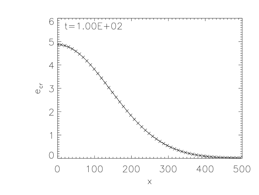
Figure 1: Comparison of numerical solutions of the 1D, pure diffusion problem to analytical solutions for $t=0$ (upper panel) and $t=100$ (lower panel). Continuous lines denote analytical solutions for different times and crosses represent numerical solutions.

4.2 Passive cosmic ray transport along an inclined magnetic field

The next test for the diffusive cosmic-ray propagation is to check if the simulated diffusion follows the analytical solution in case of an inclined magnetic field. We set up the values of $K_{\parallel}=100$ and $K_{\perp}=0$ and perform simulations for $B_{x}=B_{y}\neq 0$ and $B_{z}=0$.

Fig. 2 presents two snapshots of cosmic ray distribution at $t=0$ and $t=100$. It is apparent that qualitatively the anisotropic transport of cosmic ray energy proceeds along the magnetic field according to our expectations.

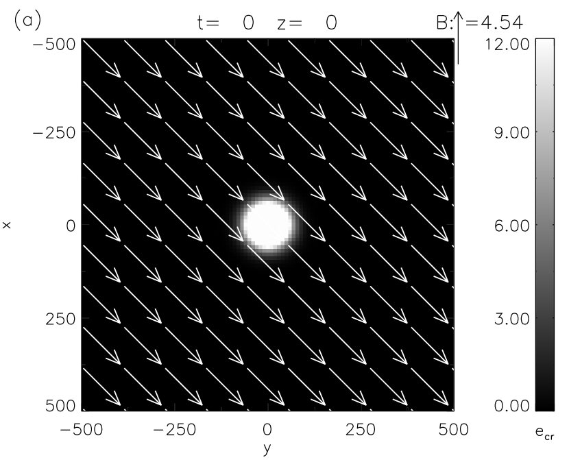
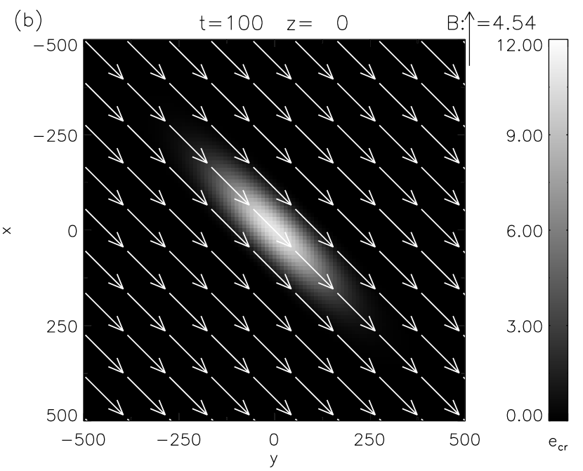
Figure 2: Diffusion of cosmic rays along an inclined magnetic field: (a) the initial spheroidal distribution of $e_{\rm cr}$ at $t=0$ and (b) the ellipsoidal distribution at $t=100$.

However, a more precise evaluation of the numerical algorithm can be performed by fitting a 2D-Gaussian function for the distribution of cosmic ray energy density in the $xy$-plane. The diffusion along the $z$-direction is absent in the current setup. The fitting procedure is performed with the aid of IDL routine gauss2dfit, which returns parameters of a 2D-Gaussian distribution, i.e the semi-axis of the ellipsoid, as well as the amplitude of the peak and the level of the constant background distribution of cosmic ray energy. The results of the fitting are shown in Fig. 3, where two 1-d slices along the major and minor axis of the ellipsoid (crosses and asterisks respectively) are shown together with the corresponding curves calculated on the base of the derived parameters of the ellipsoid.

Figure 3: Diffusion of cosmic rays along an inclined magnetic field at $t=100$. Two cuts of the ellipsoid shown in Fig. 2 are made (b) along the major axis (crosses) and along the minor axis (asterisks). The full and dotted lines represent the corresponding cuts of the fitted 2D Gaussian profile.

In the present case the fitted values of the parallel and perpendicular widths of the 2D Gaussian profile and the fitted amplitude are $r_{\parallel f}=206.429$, $r_{\perp f}=54.705$, $A_{f}=11.096$. Since $K_{\perp}=0$, the corresponding parameters of the exact solution can be derived from formula (20) representing the time evolution of 1D Gaussian profile. The exact analytical solution gives $r_{\parallel a}=\sqrt{r_{0}^{2}+4Kt}=206.155$ and $A_{a}=A/\sqrt{r_{0}^{2}+4Kt}=11.884$. If no perpendicular diffusion is present, the perpendicular widths should not change, i.e. $r_{\perp a}=50.000$.

We note that the parallel width of the 2D Gaussian profile of the simulated cosmic ray distribution coincides well with the analytical solution. However, there are two noticeable effects of the limited accuracy of our numerical algorithm. The first effect is the broadening of the perpendicular widths $r_{\perp}$ by about 10% of the original value. The broadening leads to a lowering of the peak amplitude $A_{f}$ with respect to the exact solution since the total cosmic ray energy is conserved in absence of gas flows. The second effect of the limited numerical accuracy affects the formation of regions with negative values of cosmic ray energy density at the base of steep sides of the ellipsoid.

The depth of the $e_{\rm cr}$ deficit (currently equal to $-0.09123$ at $t=100$) is strongly dependent on the grid resolution and the steepness of the initial cosmic ray energy distribution across the magnetic field lines. The presence of negative CR energy density regions may lead to significant numerical artifacts as soon as cosmic rays are coupled to the equation of gas motion. Therefore the spatial resolution of the grid in conjunction with the magnitude of the cosmic ray gradients is an issue of primary importance. The deficit vanishes in proportion to the grid resolution, however there is a limited freedom of reducing the size of the grid cell due to a drastic reduction of the timestep given by formula (17).

An alternative way is to incorporate an explicit perpendicular diffusion given by $K_{\perp}$ equal to a few up to a few 10 percent of $K_{\parallel}$. This procedure can be physically justified by studies of cosmic ray transport in turbulent magnetic fields (Giaccalone and Jokipii 1999). Another way to eliminate the spots of negative cosmic ray energy density is to add a smooth background of cosmic rays prior to the injection of very localized portions of cosmic ray energy. This is also a physically justified procedure, since e.g. the smooth background of cosmic rays is present in the ISM.

4.3 Active cosmic ray transport

After testing the passive diffusion of cosmic rays we can now describe the active propagation of cosmic rays within the overall setup similar to that of the previous subsection. In the present configuration we apply the uniform background of cosmic rays resulting from the assumption that cosmic ray pressure is equal to the magnetic and gas pressure

$$p_{\rm tot}=p_{\rm gas}+p_{\rm mag}+p_{\rm cr}$$ (21)

where

$$p_{\rm mag}=\alpha_{p}p_{\rm gas}$$ (22)

$$p_{\rm cr}=\beta_{p}p_{\rm gas}$$ (23)

and $\alpha_{\rm p}$ and $\beta_{\rm p}$ are in general constants of the order of 1 in the ISM. In the present case we adopt $\alpha_{\rm p}=\beta_{\rm p}=1$. The constant scaling factors between cosmic ray and gas background pressures as well as between magnetic and gas pressures is adopted for testing purposes only. This approach is useful especially in linear studies of Parker instability and follows the original work by Parker (1966, 1967). In general, one can start with any arbitrarily chosen initial magnetic field and cosmic ray distributions. The corresponding background cosmic ray energy density in our units is $e_{\rm cr}=(\gamma_{\rm cr}-1)^{-1}\alpha_{p}c_{\rm si}^{2}\rho_{0}=147$, where $c_{\rm si}=7{\rm\ km}{\rm\ s}^{-1}$ denotes the isothermal sound speed and $\rho_{0}=1$ is the background gas density.

In order to investigate the coupling of cosmic rays to gas and magnetic field we switch on the $\mbox{{\boldmath$\nabla$}}p_{\rm cr}$ term in the equation of gas motion and inject about 50 % of $10^{51}{\rm\ erg}$ of the kinetic output of the SN explosion. In our scaled units this corresponds to the initial peak amplitude of the Gaussian CR distribution equal to 100 times the background thermal energy density, i.e $100c_{\rm si}^{2}\rho_{0}=4900$. Currently we apply a rather small diffusion coefficient of cosmic rays $K_{\parallel}=100$ (corresponding to $3\cdot 10^{25}{\rm\ cm}^{2}{\rm\ s}^{-1}$) and $K_{\perp}=4$ in order to illustrate the effects of cosmic ray propagation qualitatively.

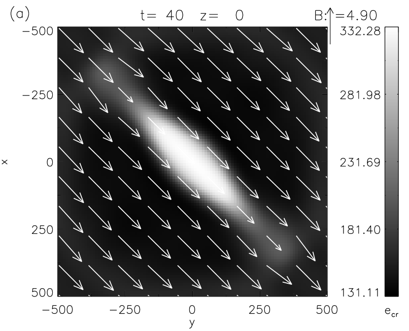
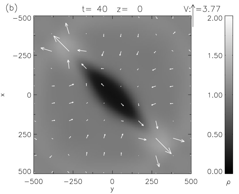
Figure 4: Diffusion of cosmic rays along an inclined magnetic field at $t=40$: (a) the cosmic ray energy density $e_{\rm cr}$ and magnetic field and (b) distribution of gas density and gas velocity.

In Fig. 4 we present the cosmic ray - magnetic field distribution (panel a) and the density - velocity distribution (panel b) at $t=40$. The difference between the passive and active cosmic ray transport is remarkable. First of all the gradient of the cosmic ray pressure leads to the acceleration of gas. Due to the effect of magnetic tension gas accelerates preferentially along the magnetic field up to a few ${\rm\ km}{\rm\ s}^{-1}$. The outflow of gas from the cosmic ray injection region together with the expansion forced by the cosmic ray pressure implies the formation of a cavity in the gas distribution. On the other hand, gas accumulates outside the cavity as it is visible in 4 (b), in the upper-left and lower-right corners of the graphic.

The gas motion along the magnetic field lines leads to an advection of cosmic rays with the gas flows, which is noticeable in Fig. 4 (a) as an enhanced cosmic ray energy density coinciding with the enhanced gas density in Fig. 4 (b). The coupling of cosmic rays to the gas component implies that the cosmic rays spread faster with respect to the passive (pure diffusion) transport. A broadening of the cosmic ray profile across the magnetic field is due to the pressure of the cosmic ray gas and partially due to the imposed perpendicular diffusion.

5 Active cosmic ray transport in a vertically stratified atmosphere

For the simulations of the cosmic ray transport in a stratified atmosphere we adopt a physical domain and grid sizes $500\times 1000\times 1000$ pc and $50\times 100\times 100$ grid zones, in $x$, $y$ and $z$ directions respectively. We apply periodic boundary conditions to all the vertical domain boundaries, a reflection boundary condition to the lower domain boundary and outflow condition to the upper boundary.

The goal of the present work is to incorporate the cosmic ray transport into studies of the dynamics of a gravitationally stratified interstellar medium. In this section we perform an experiment similar to the ones presented in the previous sections. However, in the present case a uniform vertical gravity is taken into account for the construction of an initial equilibrium state. The equilibrium fulfills the magnetohydrostatic force balance equation

$$-\frac{d{p_{\rm tot}}}{d{z}}+g_{z}=0,$$ (24)

where $p_{\rm tot}=p(1+\alpha_{p}+\beta_{p})$ denotes the total pressure and $g_{z}=-0.65{\rm\ pc}{\rm\ Myr}^{-2}$ is the vertical, uniform gravitational acceleration. The center of cosmic ray injection is placed at $x=0$, $y=0$ and $z=100$. Two slices illustrating the geometry of the initial state are shown in Fig. 5.

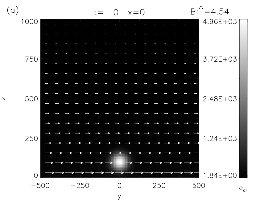
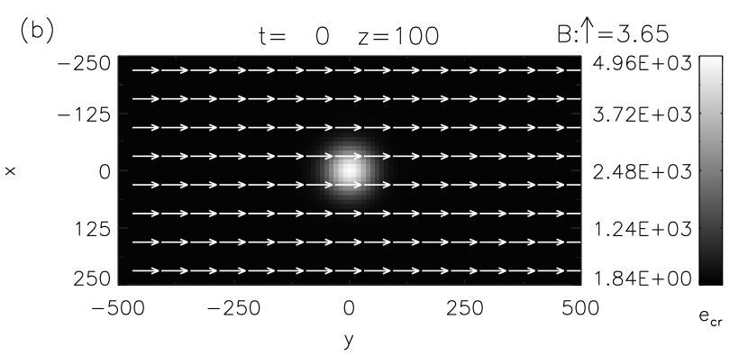
Figure 5: Geometry of the initial state stratified by vertical gravity: (a) the slice in $yz$-plane showing the stratification of the background distribution of cosmic rays and magnetic field along with the localized cosmic ray injection region, (b) the initial, horizontal magnetic field is parallel to the horizontal and parallel to the $y$-axis.

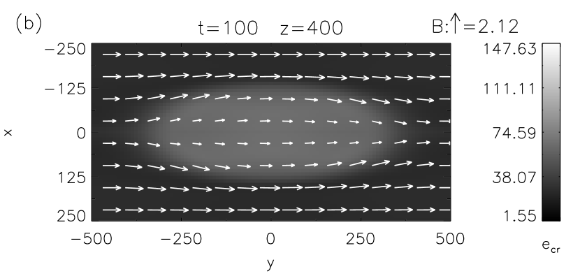
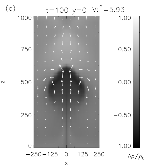
Figure 6: Propagation of cosmic rays in a vertically stratified atmosphere for the diffusion coefficient $K_{\parallel}=10^{4}$, after the local injection of cosmic ray energy: (a) cosmic ray energy density and magnetic field in the $yz$-plane at $x=0$ and (b) in the $xy$-plane at $z=400$, (c) the density perturbation $\Delta\rho/\rho_{0}$ and the gas velocity in the $xz$-plane.

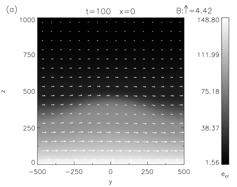
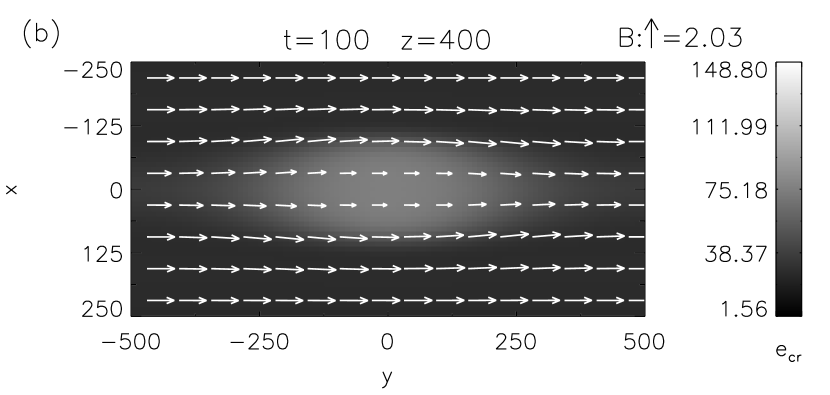
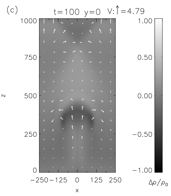
Figure 7: Same as Fig. 6 for the diffusion coefficient $K_{\parallel}=10^{5}$ at $t=100$.

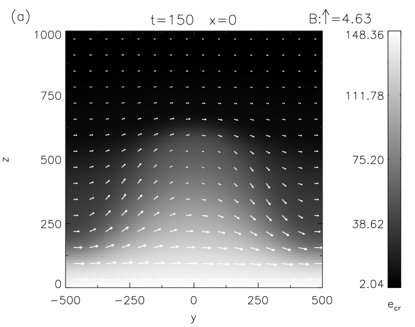
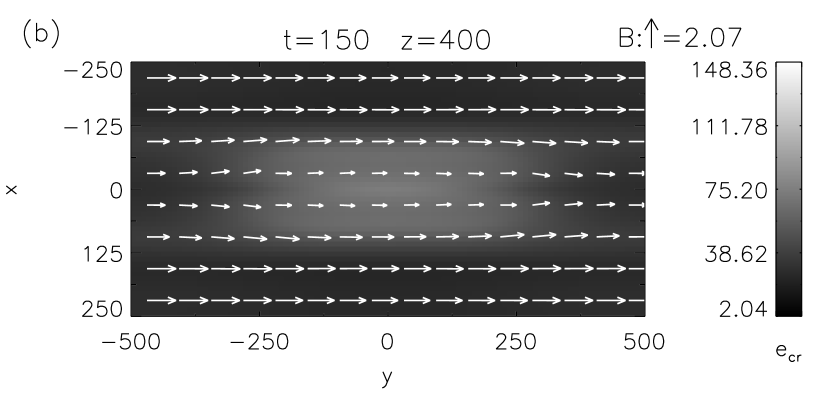
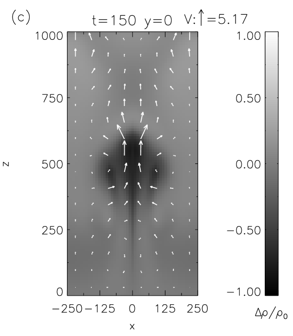
Figure 8: Same as Fig. 7 at $t=150$.

Fig. 6 shows the state of the system at $t=100$ in case of $K_{\parallel}=10^{4}$ (corresponding to $3\cdot 10^{27}{\rm\ cm}^{2}{\rm\ s}^{-1}$) and $K_{\perp}=0$. Cosmic rays injected into a localized region diffuse anisotropically along the magnetic field lines and populate a fluxtube marked by magnetic lines threading the initial injection volume. Due to an excess of cosmic ray pressure the flux tube becomes underdense and its central part starts to rise against vertical gravity. The overall evolution of the fluxtube follows closely the one described in the thin fluxtube approximation by Hanasz & Lesch (2000). The gradient of the cosmic ray pressure accelerates gas, along the direction of magnetic field, reducing additionally the gas density at the neighborhood of the injection region. That effect enhances the strength of the buoyancy force.

At $t=100$ the cosmic ray populated flux tube forms a rising Parker loop. In Fig. 6 (c) the relative density $\Delta\rho/\rho_{0}$ is shown in the $xz$-plane together with the velocity field. The apparent tube-like cavity in the density distribution results from the local excess of cosmic rays. The upward gas velocity is a consequence of the buoyancy force. The rising tube compresses the overlying gas and pushes it toward higher altitudes. The system perturbed by cosmic rays injected in a localized spherical region forms a buoyant fluxtube and evolves in a fashion resembling the development of an undulatory Parker instability mode.

When the diffusion coefficient takes a realistic value $K_{\parallel}=10^{5}$, which corresponds to $3\cdot 10^{28}{\rm\ cm}^{2}{\rm\ s}^{-1}$ the evolution of the system is remarkably different (see Figs. 7) and 8. The distribution of cosmic rays along the flux tube becomes relatively uniform before the buoyancy force starts to displace the tube in the vertical direction. The perturbation provided by the cosmic ray input excites initially (up to $t=100$) the interchange mode of the Parker instability with a weak contribution of the undulatory mode. Later on, at $t=150$, the growing contribution of the undulatory mode becomes apparent.

Due to the more efficient diffusion, cosmic rays fill in initially a larger volume, compared to the case of lower diffusion coefficient. Therefore the excess of cosmic ray pressure, and hence the buoyancy force, becomes weaker but distributed over a larger volume. At the fixed time $t=100$ after the cosmic ray injection the maximum vertical speed is smaller compared to the case of smaller diffusion coefficient $K_{\parallel}=10^{4}$, although later on the instability accelerates following the emergence of the undulatory mode. The apparent tendency seems to be opposite to that resulting from the linear stability analysis by Ryu et al. (2003). However, we point out that the lower values of the diffusion coefficient are clearly leading to stronger nonlinear effects, (for instance the vertical speed of the buoyant gas is almost equal to the sound speed). The large cosmic ray energy remains localized in a more compact region, therefore the applicability of the linear approximation for the discussed case of lower parallel diffusion coefficient ($K_{\parallel}=10^{4}$) is questionable. Despite the mentioned differences the late stages of the system for small and realistic diffusion coefficients remains rather similar.

6 Summary and conclusions

In this paper we presented a numerical algorithm for the inclusion of cosmic ray dynamics, described by the diffusion-advection equation, into the MHD code ZEUS-3D. In order to check the presented method we compared results of the diffusive passive transport of cosmic rays with analytical solutions of the diffusion equation. Our method appeared to be numerically stable in case of active transport for a wide range of diffusion coefficients, including the realistic values inferred from the observational data by Strong & Moskalenko (1998) for the Milky Way.

We applied the presented numerical algorithm to two exemplary simulations of the excitation of the Parker instability triggered by cosmic rays injected by a single SN remnant. The only difference between the input parameters of the two simulations is the magnitude of the parallel diffusion coefficient. The simulation corresponding to the realistic value of the parallel diffusion coefficient $K_{\parallel}=3\times 10^{28}{\rm\ cm}^{2}{\rm\ s}^{-1}$, presented in Figs. 7 and 8 appeared to develop the Parker instability mode slower than the one performed for $K_{\parallel}=3\times 10^{27}{\rm\ cm}^{2}{\rm\ s}^{-1}$, presented in Fig. 6. Such a tendency differs from the one resulting from linear analysis of the Parker instability by Ryu et al. (2003). We show these two examples of evolution of the system in order to demonstrate that in some circumstances the finiteness of the diffusion coefficient may lead to effects which can not be described within the simple linear approximation. Therefore a verification of all former analytical and numerical results concerning the nonlinear development of the Parker instability in presence of cosmic rays is necessary.

The presented work is just a starting point, which focuses on developing the basic computational techniques. In the next step we plan to combine the cosmic ray transport in a more realistic application by including the dynamo action of the cosmic ray component, reconfiguration of the magnetic field by magnetic reconnection, different random spatial cosmic ray source distributions and different supernova rates. The future work should also include effects of cosmic ray losses and extensions of the present algorithm to the energy dependent cosmic ray transport.

- [1] Beck, R. 2001, ‘Galactic and extragalactic magnetic fields’, Space Science Reviews, 99, 243
- [2] Berezinskii, V.S., Bulanov, S.V., Dogiel, V.A., Ginzburg, V.L., Ptuskin, V.S., Astrophysics of cosmic rays, Amsterdam: North-Holland, 1990.
- [3] Birk, G.T 2002, A&A, 391, 1155
- [4] Chou, W., Matsumoto, R., Tajima, T. Umekawa, M., Shibata, K. 2000, ApJ, 538, 710
- [5] Evans, C.R., Hawley, J.F. 1988, ApJ, 332, 659
- [6] Ferriere, K.M. 2001, ApJ, 497, 759
- [7] Ferriere, K.M. 2001, Reviews of Modern Physics, 73, 1031
- [8] Fletcher, C.A.J. 1991, Computational Techniques for Fluid Dynamics 1, Springer-Verlag
- [9] Foglizzo, T., Tagger, M. 1994, A&A, 287, 297
- [10] Foglizzo, T., Tagger, M. 1995, A&A, 301, 293
- [11] Franco, J., Kim, J., Alfaro, E., Hong, S.S. 2002, ApJ, 570, 647
- [12] Giacalone, J., Jokipii, R.J.: 1999, ApJ, 520, 204-214.
- [13] Giz, A.T., Shu, F.H. 1993, ApJ, 404, 185
- [14] Hanasz, M., Lesch, H. 1997, A&A, 321, 1007
- [15] Hanasz, M., & Lesch H. 1998, A&A 332, 77
- [16] Hanasz, M., & Lesch H. 2000, ApJ, 543, 235
- [17] Hanasz, M., & Lesch H. 2001, Space Science Reviews 99, 231
- [18] Hanasz, M., Otmianowska-Mazur, K. & Lesch H. 2002, A&A, 386, 347
- [19] Hanasz, Kosiński & Lesch 2003,
- [20] Hawley, J.F., Stone, J.M. 1995, Comput. Phys. Commun., 89, 127
- [21] Jokipii, J.R.: 1999, in J. Franco and A. Carraminana (eds.) Interstellar Turbulence, Cambridge University Press, 70-78.
- [22] Jones, T.W, Rudnick, L., Jun, B-I., Borkowski, K.J., Dubner, G. Frail, D.A., Kang, H., Kassim, N.E., McCray, R. 1998, PASP, 110, 125
- [23] Kim, J., Hong, S.S. 1998, ApJ, 507, 254
- [24] Kim, J., Hong, S.S., Ryu, D., Jones, T.W. 1998, ApJ, 506, L139
- [25] Kim, J., Franco, J., Santillan, A., Martos, M.A. 2000, ApJ, 531, 873
- [26] Kim, J., Ryu, D. 2001, ApJ, 561, L135
- [27] Kuznetsov, V.D., Ptuskin, V.S. 1983, Sov. Astron. Lett., 9, 75
- [28] Kim, W.-T., Ostriker, E.C.; Stone, J.M. 2002, ApJ, 581, 1080
- [29] Kowal, G. Hanasz, M., Otmianowska-Mazur, K. 2003, A&A (in press)
- [30] Kosinski, R., Hanasz, M. 2003, A&A (submitted)
- [31] Koyama, K.P., Petre, P., Gotthelf, E.V., et al. 1995, Nature, 378, 255
- [32] Parker, E.N. 1966, ApJ, 145, 811
- [33] Parker, E.N. 1967, ApJ, 149, 535
- [34] Ryu, D., Kim, J., Hong, S.S., Jones, T.W. 2003, Apj, 589, 338
- [35] Schlickeiser, R., Lerche, I.: 1985, A&A, 151, 151
- [36] Shu, F.H., 1974, A&A, 33, 55
- [37] Stone, J.M., Norman, M.L, 1992a, ApJS, 80, 753
- [38] Stone, J.M., Norman, M.L, 1992b, ApJS, 80, 791
- [39] Strong, A.W., Moskalenko, I.V. 1998, ApJ, 509, 212
- [40] Tanuma, S., Yokoyama, T., Kudoh, T., Shibata, K., 2003, ApJ, 582, 215