FORTE satellite constraints
on ultra-high energy cosmic particle fluxes

Abstract

The FORTE (Fast On-orbit Recording of Transient Events) satellite records bursts of electromagnetic waves arising from near the Earth’s surface in the radio frequency (RF) range of 30 to 300 MHz with a dual polarization antenna. We investigate the possible RF signature of ultra-high energy cosmic-ray particles in the form of coherent Cherenkov radiation from cascades in ice. We calculate the sensitivity of the FORTE satellite to ultra-high energy neutrino (UHE $\nu$) fluxes at different energies beyond the Greisen-Zatsepin-Kuzmin (GZK) cutoff. Some constraints on supersymmetry model parameters are also estimated due to the limits that FORTE sets on the UHE neutralino flux. The FORTE database consists of over 4 million recorded events to date, including in principle some events associated with UHE $\nu$. We search for candidate FORTE events in the period from September 1997 to December 1999. The candidate production mechanism is via coherent VHF radiation from a UHE $\nu$ shower in the Greenland ice sheet. We demonstrate a high efficiency for selection against lightning and anthropogenic backgrounds. A single candidate out of several thousand raw triggers survives all cuts, and we set limits on the corresponding particle fluxes assuming this event represents our background level.

I Introduction

Detection and modeling of the highest energy cosmic rays and the neutrinos which are almost certain to accompany them represents one of the most challenging problems of modern physics. To date a couple of tens of cosmic ray events, presumably protons, have been observed with energies in excess of 10²⁰ eV. The origin of this flux represents a puzzle since above $\sim\!5\times 10^{19}$ eV the cosmic ray flux is expected to be reduced due to Greisen-Zatsepin-Kuzmin (GZK) Greisen (1966); Zatsepin and Kuzmin (1966) mechanism. The primary particles inevitably generate ultra-high energy neutrinos (UHE $\nu$) in cosmic beam dumps. Weakly interacting neutrinos, unlike gamma photons or protons, can reach us from distant sources and therefore are a possible invaluable instrument of high-energy astrophysics.

Above $\sim 10^{19}$ eV, charged cosmic rays are no longer magnetically confined to our galaxy. This implies that particles above this energy detected at earth are very likely to be produced in extragalactic astrophysical sources. Furthermore, the existence of particles up to, and possibly beyond the $\sim 10^{19.5}$ eV endpoint of the allowed energy spectrum for propagation over cluster-scale distances suggests that there is no certain cutoff in the source energy spectra. In fact, we are unlikely to learn about the endpoint in the source energy spectra via either charged particles or photons: the universe is largely opaque to all such traditional messengers.

There are no clear physics constraints on source energy spectra until one reaches Grand-Unified Theory (GUT) scale energies near $10^{24}$ eV where particle physics will dominate the production mechanisms. If we assume that measurements at $\sim$10²⁰ eV represent mainly extragalactic sources, then there are virtually no bounds on the intervening three or four decades of energy, except what can be derived indirectly from upper limits at lower energies. For these reasons, measurements which are sensitive to ultra-high energy neutrinos are of particular importance in understanding the ultimate limits of both particle acceleration in astrophysical zevatrons (accelerators to $\sim\!\textrm{ZeV}=10^{21}$ eV and higher energies) and top-down decay of exotic forms of cosmic energy. Even at energies approaching the GUT scale, the universe is still largely transparent to neutrinos. Also, the combination of a slowly increasing cross-section combined with the large energy deposited per interaction makes such neutrino events much more detectable than at lower energies.

The chief problem in UHE $\nu$ detection arises not from the character of the events, but from their extreme rarity. For neutrinos with fluxes comparable to the extrapolated ultra-high energy cosmic ray flux at $10^{21}$ eV, a volumetric aperture of order 10⁶ km³ sr (water equivalent) is necessary to begin to achieve useful sensitivity. Such large volumes appear to exclude embedded detectors such as AMANDA AMANDA Collaboration (2000) or IceCube IceCube Collaboration , which are effective at much lower neutrino energies. Balloon-based ANITA Collaboration, S. Barwik et al. (2002) or space-based EUS ; OWL systems appear to be the only viable approaches currently being implemented.

The most promising new detection methods appear to be those which exploit the coherent radio Cherenkov emission from neutrino-induced electromagnetic cascades, first predicted in the 1960’s by Askaryan Askar’yan (1962); Askaryan (1965), and confirmed more recently in a series of accelerator experiments Gorham et al. (2000); Saltzberg et al. (2001). Above several PeV ($10^{15}$ eV) of cascade energy, radio emission from the Askaryan process dominates all other forms of secondary emission from a shower. At ZeV energies, the coherent radio emission produces pulsed electric field strengths that are in principle detectable even from the lunar surface Gorham et al. (1999, ).

These predictions, combined the strong experimental support afforded by accelerator measurements, are the basis for our efforts to search existing radio-frequency data from the Fast On-orbit Recorder of Transient Events (FORTE) satellite for candidate ZeV neutrino events. Here we report the first results of this search, based on analysis of several days of satellite lifetime over the Greenland ice sheet.

II Detector characteristics

The experiment described in this paper is based on detection of electromagnetic emission generated in the Greenland ice sheet by the FORTE satellite.

The FORTE satellite Jacobson et al. (1999) was launched on August 29, 1997 into a 70^∘ inclination, nearly circular orbit at an altitude of 800 km (corresponding to a field of view of $\sim\!27^{\circ}$ arc distance). The satellite carries two broadband radio-frequency (RF) log-periodic dipole array antennas (LPA) that are orthogonal to each other and are mounted on the same boom pointing in the nadir direction. The antennas are connected to two radio receivers of 22 MHz bandwidth and center frequency tunable in 20–300 MHz range. Beside RF receivers, the satellite carries an Optical Lightning System (OLS) consisting of a charge-coupled device (CCD) imager and a fast broadband photometer. Although for this paper we do not report analysis of optical data, in more detailed studies the optical instrument data can be used to correlate RF and optical emissions Suszcynsky et al. (2000).

The satellite recording system is triggered by a subset of 8 triggering subbands which are spaced at 2.5 MHz separations and are 1 MHz wide. The signal has to rise 14–20 dB above the noise to trigger. Typically, a trigger in 5 out of 8 subbands is required. The triggering level and algorithm can be programmed from the ground station. Multiple channels are needed for triggering because of anthropogenic noise, such as TV and FM radio stations and radars, which produce emission in narrow bands which can coincide with a trigger subband. After the trigger, the RF data is digitized in a 12-bit Data Acquisition System (DAS) at 50 Msamples/s, and the typical record length is 0.4 ms. The FORTE database consists of over 4 million events recorded in the period from September 1997 to December 1999.

The ice with its RF refraction coefficient of $n\approx 1.8$ Johari and Charette (1975) and Cherenkov angle of $\theta_{C}\approx 55.8^{\circ}$ and relatively low electromagnetic wave losses in the radio frequency range is a good medium for exploiting the Askaryan effect for shower detection. The biggest contiguous ice volume on Earth (the Antarctic) is unfortunately not available to FORTE satellite because of its orbit inclination of $70^{\circ}$. The next biggest contiguous ice volume is the Greenland ice sheet. Its area is $1.8\times 10^{6}$ km², and the depth is $\sim$3 km at the peak. However, the available depth is limited by RF losses Bogorodsky et al. (1985) to 1 km. Thus the volume of Greenland ice observed from orbit is $\approx 1.8\times 10^{6}$ km³.

III Cherenkov radio emission from particle showers

We define the electric field pulse spectrum as $\mathbf{E}(\omega)=2\int_{-\infty}^{+\infty}\mathbf{E}(t)e^{i\omega t}dt$. An empirical formula for $\mathbf{E}(\omega)$ from an electromagnetic shower in ice was obtained by Zas et al. Zas et al. (1992):

$$R|\mathbf{E}(\omega)|=1.1\times 10^{-7}\frac{\mathcal{E}_{\rm shower}}{1{\rm\ TeV}}\frac{f}{f_{0}}\frac{1}{1+0.4(f/f_{0})^{2}}\times{}$$

$${}\times e^{-\frac{(\theta-\theta_{c})^{2}}{2\Delta\theta}}{\rm\ V\,MHz^{-1}}$$ (1)

where $R$ is the distance to the observation point in ice, $\mathcal{E}_{\rm shower}$ is the shower energy, assumed to be $\lesssim$1 PeV, $f$ is the electromagnetic wave frequency, $f_{0}=500$ MHz, $\theta_{c}=55.8^{\circ}$ is the Cherenkov angle, and $\Delta\theta=2.4^{\circ}f_{0}/f$.

The FORTE detector triggers whenever the amplitude of the electric field after a narrow-band (1 MHz) filter exceeds a set threshold (in several channels). Since $|\mathbf{E}(\omega)|$ varies slowly enough in this band, the peak value of $E$ on the filter output equals $|\mathbf{E}(\omega)|\Delta f$, where $\Delta f$ and $f=\omega/(2\pi)$ are correspondingly the bandwidth and the central frequency of the filter.

For low frequencies the emission cone is broad ($\Delta\theta\sim$ radian) and the empirical formula (1) is not very accurate. Instead, we make an analytical estimate for emission in Appendix A and get

$$R|\mathbf{E}(\omega)|=\sqrt{2\pi}\mu\mu_{0}QLf\sin\theta e^{-(kL)^{2}(\cos\theta-1/n)^{2}/2}$$ (2)

where $k=2\pi nf/c$ and $n=1.8$ is the ice refraction coefficient, and $\mu=1$. At $kL\gg 1$ this formula matches the empirical formula (1) for $L\approx 1.5$ m and $Q\approx(\mathcal{E}_{\rm shower}/1{\rm\ TeV})\times 5.5\times 10^{-17}$ C, which agrees with the results of shower simulations in Figures 1, 2 in Zas et al. (1992). Equation (2) also matches the numerical result for the radiation pattern at 10 MHz (Figures 11, 12 in Zas et al. (1992)) better than the empirical formula (1) which becomes inaccurate at low frequencies.

Note that we cannot use equations (1), (2) for electromagnetic showers started by particles of high energies because of significant elongation due to Landau-Pomeranchuk-Migdal (LPM) effect Landau (1944); Landau and Pomeranchuk (1952, 1953); Migdal (1956). According to Stanev et al. (1982), the LPM effect is important for particle energies $\mathcal{E}>\mathcal{E}_{\rm LPM}$, where $\mathcal{E}_{\rm LPM}=2.4$ PeV. According to Appendix B, for electromagnetic showers with starting energy $\mathcal{E}_{0}\gg\mathcal{E}_{\rm LPM}$, the electric field at the exact Cherenkov angle is still approximately given by (1), while the width of Cherenkov cone is reduced to

$$\Delta\theta_{\rm LPM}\approx 0.9^{\circ}\frac{1}{\sqrt{\mathcal{E}_{0}/1{\rm\ EeV}}}\frac{f_{0}}{f}$$ (3)

where $f_{0}=500$ MHz. For this reason, pure electromagnetic showers (primarily from $\nu_{e}$ or $\bar{\nu}_{e}$ charged current interactions) make a negligible contribution to the FORTE sensitivity because, as we will see, the energy threshold is $\gg$1 EeV.

After the interaction with a nucleon, the UHE $\nu$ energy goes into leptonic and hadronic parts. In the case of an electron (anti-)neutrino $\nu_{e}$ ($\bar{\nu}_{e}$), the electron created in the charged current interaction starts an electromagnetic shower, which is however very elongated due to LPM effect making it virtually undetectable. In the case of a $\nu_{\mu}$ ($\bar{\nu}_{\mu}$) or $\nu_{\tau}$ ($\bar{\nu}_{\tau}$) the lepton does not start a shower. The muons and tau leptons deposit their energy due to electromagnetic Mitsui (1992) and photonuclear Bugaev and Shlepin (2003) interactions. However, the portions in which the energy is deposited are not enough to be observed by FORTE. Also, the tau lepton may decay at a long distance from its creation point after its energy is reduced to $\lesssim$1 EeV (10¹⁸ eV). Thus, tau lepton decay is also unobservable by FORTE.

On the basis of these arguments, we only consider the neutrino-initiated hadronic shower, and we do not distinguish between neutrino flavors. Most of the hadronic energy converts in the end into electromagnetic, thus Cherenkov emission as a result of Askaryan effect can be used for its detection. Moreover, the LPM effect does not produce significant shower elongation, as shown by Alvarez-Muñiz and Zas Alvarez-Muñiz and Zas (1998), since most of the $\pi_{0}$ particles which decay into photons instead of interacting have their energy reduced below the LPM level. Thus, the value of $L\approx 1.5$ m used in (2) does not change appreciably. This is in accordance with results of Monte Carlo calculations of Alvarez-Muñiz and Zas (1998), showing that the Cherenkov cone narrows by only $\sim$30% when hadronic shower energy ranges from 1 TeV to 10 EeV.

The hadronic shower energy which should be used in (1) or (2) is $\mathcal{E}_{\rm shower}=y\mathcal{E}_{\nu}$, where $\mathcal{E}_{\nu}$ is the neutrino energy, and $y$ is the fraction of energy going into the hadronic shower. The theoretical value for UHE $\nu$ is $\langle y\rangle\approx 0.2$ Gandhi et al. (1996).

Because the long wavelength observed by FORTE ($\sim$6 m in ice) are far greater than the Molière (transverse) radius of the showers involved ($\sim$11.5 cm), the transverse structure of the shower (expressed by the factor $(1+0.4(f/f_{0})^{2})^{-1}$ in (1)) is neglected in our analysis. The same argument applies to transverse non-uniformities of hadronic showers.

IV Search for relevant signals in the FORTE database

IV.1 Geographic location of FORTE events

The geographic location of the signal source can be determined using the dispersion of the short electromagnetic pulse in HF range going through ionosphere. Two important parameters used in geolocation of the source can be determined from the data from a single FORTE antenna. The first parameter is the total electron content (TEC) along the line-of-site between the source and the satellite. It is proportional to the group time delay, which has $f^{-2}$ frequency dependence Tierney et al. (2001). The second parameter is determined from the Faraday rotation of a linearly polarized signal Jacobson and Shao (2001), due to birefringence in magnetoactive ionospheric plasma. The Faraday rotation frequency turns out to be equal to the “parallel” electron gyrofrequency $f_{\parallel,ce}=eB_{\parallel}/m_{e}=f_{ce}\cos\theta$, where $\theta$ is the angle between the geomagnetic field $\mathbf{B}$ and the ray trajectory at the intersection with ionosphere. Both frequency-dependent delay and frequency splitting due to Faraday rotation are well seen in Figure 1. The Cherenkov radio emission is expected to be completely band-limited and linearly polarized, which enables us to make use of the second parameter for geographic location.

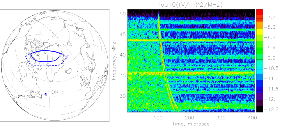
Figure 1: An example of a highly-polarized impulsive event detected by FORTE. The confidence levels for event location 67% and 90% determined using equation (4) are shown in the map. The spectrogram shows the dispersion of the pulse in the ionosphere and splitting due to Faraday rotation in geomagnetic field. The horizontal lines are due to anthropogenic noise (TV and FM radio stations).

We calculate the probability distribution of the source location using Bayesian formula:

$$p(\{\lambda,\phi\}|\mathrm{TEC},f_{\parallel,ce})=Cp(\mathrm{TEC}|\{\lambda,\phi\})p(f_{\parallel,ce}|\{\lambda,\phi\})$$ (4)

where $\{\lambda,\phi\}$ are the latitude and longitude of the source, $p(\mathrm{TEC}|\{\lambda,\phi\})$ and $p(f_{\parallel,ce}|\{\lambda,\phi\})$ are conditional probability distributions for the measured parameters given the location of the source, and $C$ is a normalization constant. Here we assume that the measurements of parameters are independent, and the a priori distribution of the source location is uniform in the field of view of the satellite.

To estimate TEC between the source and the satellite (for given locations of both), we use the Chiu ionosphere model Ching and Chiu (1973), adapted to IDL from the FORTRAN source code found at NASA ionospheric models web site. This model gives electron density as a function of altitude for given geographic and geomagnetic coordinates, time of year, time of day and sunspot number. By integrating it over altitudes, we find the vertical TEC. To convert it to TEC along the line-of-sight, we must divide it by the cosine of the angle with the vertical. Due to the curvature of the Earth, this angle is not constant along the line-of-sight, and we make an approximation of taking this angle at the point where the line-of-sight intersects the maximum of the ionosphere ($F$-layer), at altitude of $\sim$300 km. The Chiu model, due to simplifying assumptions, does not account for stochastic day-to-day variability of the vertical electron content. The standard deviation can be as large as 20–25% from the monthly average conditions (Jursa, 1985, p. 10-91). Thus, we assume a Gaussian probability distribution for $p(\mathrm{TEC}|\{\lambda,\phi\})$ with the center value calculated using Chiu model and variance of 25%.

The geomagnetic field is estimated from a simple dipole model (Jursa, 1985, pp. 4-3, 4-25). The error is assumed to be 10% according to the estimates for experimental determination of $f_{\parallel,ce}$ from the RF waveform, in Figure 6 of Jacobson and Shao (2001). However, this uncertainty can be greater for signals that are only partially linearly polarized. Again, we use a Gaussian distribution for $p(f_{\parallel,ce}|\{\lambda,\phi\})$ with corresponding central value and the standard deviation of 10%.

IV.2 Background rejection

The pulse generated by a UHE $\nu$ shower in ice is expected to be highly polarized and essentially band-limited up to a few GHz. In these aspects, it is similar to the electromagnetic emission from the “steps” in a stepped-leader lightning Jacobson and Light (2003). However, the pulses corresponding to lightning steps are accompanied by similar neighbors before and after, within a time interval from a fraction of a ms to $\sim$0.5 s. The signal grouping can thus be used to distinguish UHE $\nu$ signatures from most lightning events. Also, the lightning activity must be present, which is extremely rare in areas of the Earth covered by ice, and thus can be excluded using the method described in Section IV.1.

There is a special type of intracloud lightning which produces isolated events which are called compact intracloud discharges (CID) Smith (1998). However, these events are usually randomly polarized and have several-$\mu$s pulse durations Jacobson and Light (2003).

Another rejection method uses the fact that the lightning discharges occur above ground, and therefore there is a large probability for FORTE to detect also the signal reflected from the ground. This phenomenon is known as Trans-Ionospheric Pulse Pairs (TIPPs) Holden et al. (1995); Massey and Holden (1995); Massey et al. (1998). The presence of a second pulse, therefore, excludes the possibility of the signal to be a UHE $\nu$ signature. An example of a TIPP event in FORTE data is shown in Figure 2.

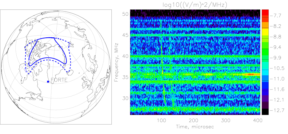
Figure 2: A TIPP (pulse pair) event with probable origin location in Greenland but rejected in our analysis. Notations are the same as in Figure 1.

V FORTE satellite sensitivity to neutrino flux

In this section, we estimate the upper limit of the differential flux of UHE $\nu$ (all flavors) depending on the number of triggers on the relevant events in the satellite lifetime. The limits are set on the sum of all flavors since this experiment cannot distinguish between them.

The typical natural background noise level in FORTE data is $\sim$10^-12–10^-11 (V/m)²/MHz (as can be seen, e.g., from spectrograms in this paper’s Figures). In a typical 1-MHz trigger subband this corresponds to RMS value of 1–3 $\mu$V/m. The trigger level is set 14–20 dB above the noise, giving the ability to trigger on impulsive signals with frequency domain values of 5–30 $\mu$V/m in each 1 MHz trigger subband. For flux limits calculations in this section, we use the threshold value of 30 $\mu$V m^-1 MHz^-1 at $f=38$ MHz, the central frequency of the low FORTE band.

V.1 Relation between FORTE sensitivity and the limits on UHE $\nu$ flux

Let $\lambda(\mathcal{E})$ be the theoretical number of triggers of FORTE satellite in its full lifetime assuming a unit monoenergetic neutrino flux for different energies $\mathcal{E}$. We will call this function the sensitivity of the FORTE satellite to UHE $\nu$ flux. Then the expected number of triggers is

$$s=\int\lambda(\mathcal{E})\Phi(\mathcal{E})d\mathcal{E}$$

where $\Phi(\mathcal{E})$ is the differential neutrino flux (per unit area, time and solid angle). The number of detected events is a Poisson distributed random number with expectation $s$. If no events are detected (null result) we can set a limit on $s$:

$$s\leq s_{\rm up}=-\log\alpha$$

where $1-\alpha$ is the confidence level. For 90% confidence level, for example, we have

$$\int\lambda(\mathcal{E})\Phi(\mathcal{E})d\mathcal{E}\leq s_{\rm up}\approx 2.3$$ (5)

In general, for $n$ events, the limiting value of $s$ is determined from

$$\alpha=Q(n+1,s_{\rm up})$$ (6)

where $Q(n+1,s_{\rm up})=\frac{\int_{s_{\rm up}}^{\infty}x^{n}e^{-x}dx}{\int_{0}^{\infty}x^{n}e^{-x}dx}$ is the regularized incomplete gamma function. For example, at a confidence level of 90% and $n=1$ we get $s_{\rm up}\approx 3.89$.

From the limit set on integrated flux (5) one can try to construct a limit on a differential flux. However, such a limit can be evaded for differential flux models that are anomalous, for example, if there are very narrow emission lines in the spectrum. Nevertheless, for reasonable assumptions such as a smooth and continuous model spectrum, the implied limits are model-independent. As shown in Appendix C, if we assume that the spectrum is sufficiently smooth, i.e. does not have any sharp peaks (the peaks have widths at least of the order of the central energy of a peak), then we can assert that

$$\Phi(\mathcal{E})\lesssim\frac{s_{\rm up}}{\mathcal{E}\lambda(\mathcal{E})}$$ (7)

Since this limit does not assume any particular model (except that it is sufficiently smooth), we will define it as the model-independent limit.

V.2 Sensitivity calculation

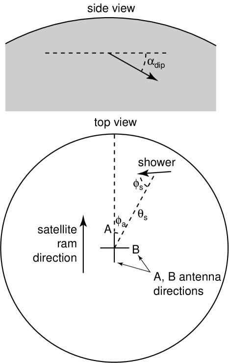
Figure 3: Configuration for sensitivity calculations.

The sensitivity $\lambda(\mathcal{E}_{\nu})$, which was introduced in the previous subsection, is calculated using the specific aperture $R$, which we define as the trigger rate for unit monoenergetic neutrino flux when neutrinos interact under a unit area of ice. The specific aperture $R$ is integrated over the visible ice area averaged over time (many satellite passes) and multiplied by the entire satellite lifetime in orbit $T$ (while the two radio receivers of 22 MHz band were in order) and the fraction of time in trigger mode (duty cycle) $D$:

$$\lambda(\mathcal{E}_{\nu})=DT\left\langle\int_{A_{\rm visible}}R(\theta_{s},\phi_{a};\mathcal{E}_{\nu})\,dA\right\rangle_{\rm time}$$

The lifetime of FORTE $T$ is from September 1997 till December 1999. The time when the emission from the Greenland ice sheet is visible by the satellite can be estimated by calculating the total time spent by FORTE inside a circle of radius $20^{\circ}$ arc distance from the approximate geographic center of Greenland, at $70^{\circ}$N, $40^{\circ}$W. This time is estimated to be $\sim$38 days. The duty cycle $D$ is estimated to be 6% by calculating the run time fraction within this circle, making the effective time of observation to be $\sim$3 days.

The specific aperture $R$ is a function of the position of the neutrino-generated shower which is given by the arc distance to the shower location $\theta_{s}$ and its azimuthal angle $\phi_{a}$ (see Figure 3). Note that the visible area $A_{\rm visible}$ depends on the satellite location. Averaging over time in our calculations is replaced by averaging over satellite position over the Earth surface with a weight corresponding to the fraction of time the satellite spends in a given point of the globe.

To calculate the specific aperture $R$, we must calculate how many neutrinos interact in ice, depending on energy $\mathcal{E}_{\nu}$, dip angle $\alpha_{\rm dip}$ (the angle of $\nu$ velocity below the horizon at the interaction point) and the depth of interaction $z$. We use the theoretical neutrino-nucleon interaction cross-section $\sigma_{\nu N}(\mathcal{E}_{\nu})$ Kwiecinski et al. (1999). The neutrino flux from below is greatly reduced by interactions in the Earth volume, and most detectable interactions are from horizontal and down-going events. Here we have to note that this statement does not apply to neutralino interactions since neutralino-nucleon interaction cross-section $\sigma_{\chi N}$ can be much smaller than neutrino cross-section at a similar energy Barbot et al. (2003).

The number of interactions in ice is characterized by function $F(\Omega,z;\mathcal{E}_{\nu})$ defined in the following way:

$$\Phi F(\Omega,z;\mathcal{E}_{\nu})\,d\Omega\,dV=N_{\rm nuc}\sigma_{\nu N}(\mathcal{E}_{\nu})\,d\Phi\,dV$$

Here $\Omega=(\alpha_{\rm dip},\phi_{s})$ is the neutrino velocity direction (see Figure 3), $z$ is the interaction depth, $N_{\rm nuc}$ is the nucleon number density and $d\Phi=\Phi e^{-\tau}d\Omega$ is the flux in solid angle element $d\Omega=\sin\alpha_{\rm dip}d\alpha_{\rm dip}d\phi_{s}$ attenuated by neutrino absorption in a layer of optical thickness $\tau(\alpha_{\rm dip},z)=\int N_{\rm nuc}\sigma_{\nu N}dl$.

The specific aperture $R$ is found using the fraction of interacting neutrinos which produce field $E_{\rm ant}>E_{\rm th}$ at the satellite antennas:

$$R(\theta_{s},\phi_{a};\mathcal{E}_{\nu})=\int F(\Omega,z;\mathcal{E}_{\nu})$$

$$\left(\int_{0}^{1}\Theta[E_{\rm ant}(y\mathcal{E}_{\nu},\Omega,\theta_{s},\phi_{a})-E_{\rm th}]p(y)\,dy\right)\,d\Omega\,dz$$

where $\Theta$ is the step function, and $p(y)=(1/\sigma)(d\sigma/dy)$ is the probability distribution function for the kinematic parameter $y=\mathcal{E}_{\rm had}/\mathcal{E}_{\nu}$, the fraction of energy going into the hadronic shower. The $p(y)$ dependence is taken from Gandhi et al. (1996) for the highest energy considered in that paper, $\mathcal{E}_{\nu}=10^{12}$ GeV. Since $E_{\rm ant}(y\mathcal{E}_{\nu},\Omega,\theta_{s},\phi_{a})=yE_{\rm ant}(\mathcal{E}_{\nu},\Omega,\theta_{s},\phi_{a})$, we can integrate over $y$ immediately and get

$$R(\theta_{s},\phi_{a};\mathcal{E}_{\nu})=\int F(\Omega,z;\mathcal{E}_{\nu})$$

$$\left[1-F_{y}\left(\frac{E_{\rm th}}{E_{\rm ant}(\mathcal{E}_{\nu},\Omega,\theta_{s},\phi_{a})}\right)\right]d\Omega dz$$

where $F_{y}(y)=\int_{0}^{y}p(y^{\prime})dy^{\prime}$ is the cumulative distribution function of $y$.

Given a neutrino interacting at dip angle $\alpha_{\rm dip}$ and depth $z$ in ice, we can calculate the field detected at the satellite. First, the emitted field is given by Cherenkov emission formula (2). Then the field is attenuated in ice, refracted at the ice surface and detected at the satellite taking into account the directional antenna response. In the subsections of Appendix D, we give the details of calculations for these steps. In Figure 4, we show the peak electric field at the satellite altitude (800 km) at the central frequency of the low FORTE band ($f=38$ MHz). As we see, even for a dip angle of $20^{\circ}$ there is a significant emission upward from the shower due to the width of Cherenkov cone. Although the field plotted in Figure 4 does not include the antenna response, the plots can give some idea about where the satellite has to be to see the signal at a given threshold, the typical value of the threshold being 30 $\mu$V m^-1 MHz^-1.

Figure 4: The peak electric field at the satellite altitude $E_{\rm sat}$, emitted in a Cherenkov process by a hadronic shower of energy $2\times 10^{22}$ eV. These plots do not include the antenna response. The shower is in the center of the circle, and is directed to the right. Emission is shown for interaction at depth $z=100$ m and dip angles of (a) $\alpha_{\rm dip}=0^{\circ}$ and (b) $\alpha_{\rm dip}=20^{\circ}$. The dashed circles represent the arc distance in degrees ($1^{\circ}\approx 111$ km on the Earth surface).

VI Results

VI.1 Event search results

We searched for events recorded while FORTE was inside a circle of radius of 20^∘ with a center at 70^∘N, 40^∘W, in time period from the start of FORTE in September 1997 to December 1999, when both 22-MHz-bandwidth receivers were lost Roussel-Dupré et al. (2001). We estimate that the satellite spent a total of 38 days inside this circle, with at least $\sim$6% of it being the time in trigger mode. We found a total of 2523 events. From these, only 77 are highly polarized. These 77 events can be geolocated using both parameters described in subsection IV.1. Of these, only 16 events have intersection of the 90% confidence level with Greenland’s ice sheet. Out of the remaining 16 events, 11 are rejected for being TIPP events, i.e. pulse pairs with ground reflections that indicate that the origin locations are above ground. An example of a rejected TIPP event is shown in Figure 2. Two more events were rejected because of the presence of a precursor before the pulse, which is characteristic of certain type of lightning Jacobson and Shao (2002) and cannot be present in a neutrino shower signal. An example of such event was shown in Figure 1.

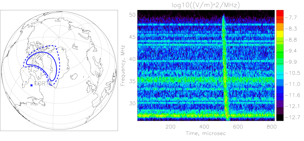
Figure 5: The confidence levels of 67% and 90% for geographic location and a spectrogram of an example event. This event cannot be generated by a neutrino due to its long duration ($\gtrsim$10 $\mu$s).

Out of the remaining three events, one (shown in Figure 5) is rejected for its long duration ($\gtrsim$10 $\mu$s), since the Cherenkov pulse is expected to be only $\sim$1 ns long (the time resolution of the FORTE detector limits this to $\gtrsim$20 ns). The remaining two events are shown in Figures 6 and 7. The first of them has close neighbor events (at $-1.4$ ms and $+0.7$ ms), which makes it a probable part of a stepped-leader process in a lightning. The neighbors of the second event are not very close (at $-0.27$ s and $+5.55$ s), but it still can be a lightning event. The recent analysis by the FORTE team Jacobson and Light (2003) has shown that the lightning events are likely to have neighbors in $\pm 0.5$ s interval, with the most probable separation of $\pm 0.01$ s, and the accidental coincidence rate is $\sim$0.9 per second. This value of the accidental coincidence rate makes the candidate event shown in Figure 7 indistinguishable from an isolated lightning discharge. The analysis of this event continues.

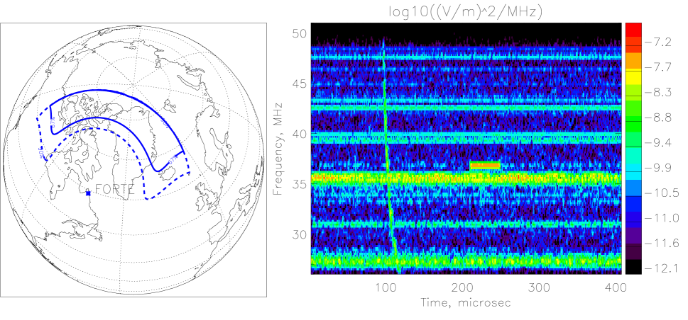
Figure 6: The confidence levels of 67% and 90% for geographic location and a spectrogram of an example event. A short horizontal streak in the spectrogram is due to anthropogenic noise (a radar). This event needs further consideration for being rejected as neutrino-generated. However, its nearest neighbor events were found at $-1.4$ ms and $+0.7$ ms, which makes it a probable lightning event.

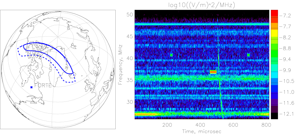
Figure 7: The confidence levels of 67% and 90% for geographic location and a spectrogram of an example event. Its nearest neighbors were found at $-0.27$ s and $+5.55$ s. This event needs further consideration for being rejected as neutrino-generated.

VI.2 Flux limits set by FORTE

In Table 1 we give the calculated FORTE neutrino flux sensitivity values $\lambda(\mathcal{E}_{\nu})$. On the basis of these values one can set a limit on any model flux $\Phi(\mathcal{E}_{\nu})$ using numerical integration in equation (5), with $s_{\rm up}=3.89$ since we have one uncertain event as our background noise. In Figure 8 we plot the model-independent flux limits set by equation (7) on the basis of these data (again with $s_{\rm up}=3.89$). In the same Figure we also show the comparison of calculated flux limits with predicted neutrino fluxes from various sources. Some of the sources of super-GZK neutrinos are reviewed, e.g. in Berezinsky (2003). As we see, the flux limits set by FORTE observations of the Greenland ice sheet can reject some regions of parameters of the Z burst model Fargion et al. (1999); Weiler (1999, 2001); Gelmini and Kusenko (2000); Fodor et al. (2002a, b).

Table 1: The FORTE sensitivity $\lambda(\mathcal{E})$ (cm² s sr) to neutrino flux (any neutrino flavor) and neutralino flux (for different neutralino-nucleon cross-sections).

$\log_{10}\mathcal{E}$	$\lambda(\mathcal{E}_{\nu})$	$\lambda(\mathcal{E}_{\chi})$	$\lambda(\mathcal{E}_{\chi})$	$\lambda(\mathcal{E}_{\chi})$
(GeV)		$\sigma_{\nu N}$	$0.1\sigma_{\nu N}$	$0.01\sigma_{\nu N}$
13.0	$8.0\times 10^{12}$	$2.1\times 10^{14}$	$2.6\times 10^{13}$	$4.1\times 10^{12}$
13.5	$5.4\times 10^{14}$	$5.6\times 10^{15}$	$6.6\times 10^{14}$	$7.9\times 10^{13}$
14.0	$5.3\times 10^{15}$	$3.2\times 10^{16}$	$3.8\times 10^{15}$	$4.3\times 10^{14}$
14.5	$2.4\times 10^{16}$	$9.7\times 10^{16}$	$1.2\times 10^{16}$	$1.3\times 10^{15}$
15.0	$7.1\times 10^{16}$	$2.2\times 10^{17}$	$2.8\times 10^{16}$	$3.0\times 10^{15}$
15.5	$1.7\times 10^{17}$	$4.1\times 10^{17}$	$5.6\times 10^{16}$	$6.1\times 10^{15}$
16.0	$3.4\times 10^{17}$	$6.9\times 10^{17}$	$1.0\times 10^{17}$	$1.1\times 10^{16}$
16.5	$6.0\times 10^{17}$	$1.0\times 10^{18}$	$1.7\times 10^{17}$	$1.9\times 10^{16}$
17.0	$9.5\times 10^{17}$	$1.4\times 10^{18}$	$2.6\times 10^{17}$	$3.0\times 10^{16}$

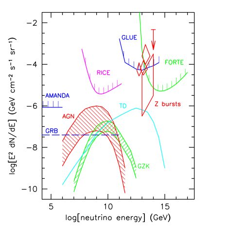
Figure 8: The estimated limits on UHE $\nu$ flux detectable by FORTE using Greenland ice sheet. The limit is compared to predicted neutrino fluxes from various sources: GRB: gamma ray bursts Waxman and Bahcall (1997); AGN: active galactic nuclei Mannheim (1995); GZK: neutrinos produced in GZK mechanism from cosmic rays Hill and Schramm (1985); TD: topological defect model (non-SUSY) Sigl et al. (1999); Z burst models are: the slanted box by Weiler (2001), the diamonds showing the 1$\sigma$ level errors are by Fodor et al. (2002b); Ringwald , and the arrow is by (Gelmini and Kusenko, 2000, default value of parameters). The limits from other experiments are also shown: AMANDA AMANDA Collaboration (2003), RICE RICE Collaboration, I. Kravchenko et al. (a) (determined using (7) from the effective volume and time of observation), GLUE Gorham et al. (1999, ). The limits from all experiments show the limits on the combined flux of neutrinos of all flavors (assumed mixed in equal amounts), except AMANDA which is only sensitive to $\nu_{\mu}$ ($\bar{\nu}_{\mu}$).

Note that differential fluxes in some models can be even smoother and wider in energies than assumed for derivation of (7). Figure 9 shows what would be the limits on a class of models with power-law energy dependence of the flux, $\Phi(\mathcal{E})\propto\mathcal{E}^{-\alpha}$. A similar analysis using power-law models was performed in the past, e.g., for RICE detector RICE Collaboration, I. Kravchenko et al. (b).

Figure 9: Upper curve: the differential flux limit of equation (7); lower set of lines: the limits set by equation (8) assuming power law flux shapes $K(\mathcal{E};\alpha)=\mathcal{E}^{-\alpha}$ for $\alpha$ in the interval from $1.6$ to $6.0$ with a step of $0.4$.

As another result of present research, we set limits on the flux of neutralinos, weakly interacting particles predicted by the Minimal Supersymmetric Standard Model (MSSM). The calculations are performed in the same way as for setting the neutrino flux limits with a few differences. First, the cross-section for nucleon interaction $\sigma_{\chi N}$ is different, and is expected to be in the range from $\sim\!(1/100)\sigma_{\nu N}$ to $\sim\!\sigma_{\nu N}$ Barbot et al. (2003). Second, all of the energy goes into the hadronic shower. The results are presented also in Table 1. In Figure 10, we compare the predicted neutralino fluxes Barbot et al. (2003) with the model-independent flux limits set by FORTE. We see that for neutralino-nucleon cross-sections in the range $\sigma_{\chi N}\gtrsim 0.1\sigma_{\nu N}$, strong limits are set on the model predicting neutralino flux from decay of heavy $X$ particles with $M_{X}=2\times 10^{25}$ eV, especially if the sources are homogeneously distributed. Note that for a case of a different mass, $M_{X}=2\times 10^{21}$ eV, which is also considered in Barbot et al. (2003), we are unable to set any limits since all decay products are below FORTE threshold.

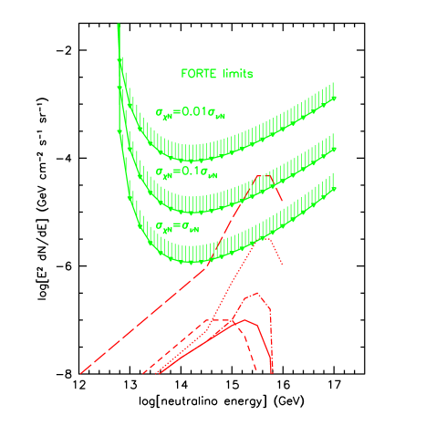
Figure 10: The limits on neutralino fluxes set by FORTE observations of the Greenland ice sheet, for one detected event and different assumptions about neutralino-nucleon cross-sections. Shown also are predicted neutralino fluxes Barbot et al. (2003) for decay of superheavy particles of $M_{X}=2\times 10^{25}$ eV. The lower four curves are for $X$ decays in the halo of the Galaxy, with the primary decay into: (1) quark$+$antiquark (solid); (2) quark$+$squark (dot-dash); (3) $SU(2)$ doublet lepton$+$slepton (dots); (4) 5 quark$+$5 squark (short dashes). The upper curve (long dashes) is for homogeneous $X$ distribution (in which case the flux is enhanced by a factor of 15 compared to a “galactic” distribution), decay scenario 3. See also Table 2.

In Table 2, we apply the more robust model-dependent limit to these models to get the confidence level of rejection according to equation (6), for $n=1$ (one uncertain event). We vary cross-section $\sigma_{\chi N}$, take different decay scenarios and $X$ distributions. As one can see from this Table, several models are rejected with very high confidence.

Table 2: The confidence levels for rejecting the models of neutralino production by heavy $X$ particle decay with $M_{X}=2\times 10^{25}$ eV Barbot et al. (2003). We only show models with the rejection confidence level $>$50%. The scenarios of $X$ decay are the same as in Figure 10. The variable $\alpha$ is defined as $1-\textrm{CL}$.

$\sigma_{\chi N}/\sigma_{\nu N}$	decay scenario	$X$ distribution	expected number of triggers	$\alpha$	CL
1	1	homogeneous	8.2927	$2.3264\times 10^{-3}$	99.7674%
1	2	homogeneous	14.0678	$1.1708\times 10^{-5}$	99.9988%
1	3	halo	6.7491	$9.0814\times 10^{-3}$	99.0919%
1	3	homogeneous	101.2365	$1.1044\times 10^{-42}$	100%
1	4	homogeneous	11.6834	$1.0696\times 10^{-4}$	99.9893%
0.1	2	homogeneous	1.8251	$4.554\times 10^{-1}$	54.4602%
0.1	3	homogeneous	13.6869	$1.6702\times 10^{-5}$	99.9983%

VII Discussion

The limits shown in Figures 8 and 10 represent to our knowledge the first direct experimental limits on the fluxes of neutrinos and other weakly interacting particles in this energy range. The fact that the first such limits already have constrained several proposed models is an indication of the power of the radio detection techniques, but the scarcity of other limits in this regime also suggests that they be accepted with caution. Here we discuss briefly some of the potential issues with these constraints.

At the energies to which FORTE is sensitive, the energy of the pulsed coherent radio emission can become one of the dominant energy-loss mechanisms for the shower. This implies that the radiation reaction of the shower to the pulse could lead to modification of the shower development, and consequently some change in the radiation parameters. We have not attempted to correct for this effect in our analysis, but we note that it is probably not important below $\sim 10^{24}$ eV Gorham et al. (2000). Above this energy we expect that the shower radiation pattern might spread to some degree, depending on the foreshortening of the cascade length due to radiation reaction deceleration.

We have noted that our limits extend into the mass scale for GUT particles. However, it is important to note that the center-of-momentum energies for interactions of these neutrinos on any other standard particles are of order 10 PeV or less. Our results thus depend on a $\leq$3 order of magnitude extrapolation of the standard model neutrino cross sections from the current highest energy estimate from accelerators at $\sim$30 TeV H1 Collaboration, I. Abt et al. (1993); ZEUS Collaboration, M. Derrick et al. (1993, 1995), over an energy regime where the cross sections grow only logarithmically with energy. For this reason we do not expect that the energy scale itself is good cause to doubt the values for the flux limits.

At 10 PeV center-of-momentum energies, interactions of the primary neutrinos will exceed in CM energy those of any observed ultra-high energy cosmic rays, and could therefore lead to production of new heavy particles in the showers themselves. Such interactions could include channels in which most of the energy goes into an unobservable particle, or a particle with interactions much weaker than neutrinos. In the absence of any specific proposals for models and interactions, we can only note that such behavior can evade our limit, but could lead to other observable secondary particles with different angular distributions that we have not considered.

Since FORTE threshold for detection of a weakly interacting particles ($\sim\!10^{22}$ eV) is higher than the GZK limit ($\sim\!5\times 10^{19}$ eV), it sets the limits on neutrinos producing super-GZK cosmic rays through resonant interaction with background neutrinos within $\sim$50 Mpc distance from us, the Z burst mechanism Fargion et al. (1999); Weiler (1999, 2001); Gelmini and Kusenko (2000); Fodor et al. (2002a, b). Although FORTE sets limits on parameters of Z burst models, the uncertainties in the models and the measured super-GZK cosmic ray flux still make most Z burst scenarios consistent with FORTE data.

The strong FORTE constraints on the neutralino production model Barbot et al. (2003) from heavy $X$ particles, sets a joint limit on (1) $X$ particle distribution and mass (2) $X$ particle decay channels and (3) neutralino-nucleon cross-section. Since some of $X$ particle decay scenarios (at the mass $2\times 10^{25}$ eV) are strongly rejected, as shown in Figure 10 and Table 2, this can give an insight into the possible nature of such particles and the physics at supersymmetric grand-unification scale. Although reference Barbot et al. (2003) does not consider models with masses intermediate between $2\times 10^{21}$ and $2\times 10^{25}$ eV, we expect that FORTE’s sensitivity, which extends an order of magnitude or more below the region where the model at $2\times 10^{25}$ is constrained, will also limit neutralinos of masses down to $\sim\!10^{24}$ eV, particularly if the cross sections approach $\sigma_{\nu N}$.

VIII Conclusions

We have performed a search for radio frequency signatures of ultra-high energy neutrinos originating from coherent Cherenkov emission from cascades in the Greenland ice sheet, observed with the FORTE satellite over an $\sim$2 year period. In $\sim$3 days of net exposure, a single candidate, presumed to be background, survives the analysis, and we set the first experimental limits on neutrino fluxes in the $10^{22}$–$10^{25}$ eV energy region. These limits constrain the available parameter space for the Z burst model. In addition we constrain several variations of a model which involves light super-summetric particles (neutralinos) at these energies, particularly those with interaction cross-sections approaching those of neutrinos.

Appendix A Cherenkov emission from electromagnetic showers

Let us model the shower as a point charge moving with the speed of light. Then the current is given by $J_{z}(\mathbf{r},t)=cq(z)\delta(\mathbf{r}-c\hat{z}t)$ and $J_{x}=J_{y}=0$. The Fourier transform is

$$J_{z}(\mathbf{r},\omega)=2\int J_{z}e^{i\omega t}dt=2q(z)\delta(x)\delta(y)e^{i\omega z/c}$$

(The factor of 2 is for consistency with our definition of $E(\omega)$) The frequency-domain vector potential $\mathbf{A}$ satisfies Helmholtz equation $\nabla^{2}A_{z}+k^{2}A=-\mu\mu_{0}J_{z}$ and $A_{x}=A_{y}=0$, where $k=n\omega/c$ and $n=\sqrt{\epsilon\mu}$. Its solution at the observation point $\mathbf{R}$ is

$$A_{z}(\mathbf{R})=\mu\mu_{0}\int\frac{e^{ikR^{\prime}}}{4\pi R^{\prime}}J_{z}(\mathbf{r})d^{3}\mathbf{r}$$

where $R^{\prime}=|\mathbf{R}-\mathbf{r}|$. In the Fraunhofer zone, the standard approximation is

$$\frac{e^{ikR^{\prime}}}{4\pi R^{\prime}}\approx\frac{e^{ikR}}{4\pi R}e^{-i(\mathbf{k}\cdot\mathbf{r})}$$

Thus,

$$A_{z}(\mathbf{R},\omega)=\mu\mu_{0}\frac{e^{ikR}}{2\pi R}\int_{-\infty}^{+\infty}q(z)e^{-iz(k\cos\theta-\omega/c)}dz$$

where $\theta$ is the emission angle.

The magnetic induction is $\mathbf{B}=\nabla\times\mathbf{A}$. In the far zone $B=|\mathbf{B}|=kA_{z}\sin\theta$ and the electric field is $E=cB/n=\omega A_{z}\sin\theta$.

Let us consider a Gaussian shower profile $q(z)=Qe^{-\frac{z^{2}}{2L^{2}}}$, where $Q$ is the maximum attained charge excess and $L$ is the characteristic shower length. Then

$$R|\mathbf{E}(\omega)|=\frac{\mu\mu_{0}QL\omega}{\sqrt{2\pi}}\sin\theta e^{-(kL)^{2}(\cos\theta-1/n)^{2}/2}$$

Appendix B Cherenkov emission from LPM showers

According to Stanev et al. (1982), LPM effect is important for particle energies $\mathcal{E}>\mathcal{E}_{\rm LPM}$, where $\mathcal{E}_{\rm LPM}=61.5X_{0}$ TeV, where $X_{0}$ is the radiation length in cm. The radiation length in mass units is 36.1 g/cm² in water, giving $X_{0}=39.1$ cm in ice since $\rho_{\rm ice}=0.924$ g cm^-3. Thus, $\mathcal{E}_{\rm LPM}=2.4$ PeV. The increased radiation length for bremsstrahlung and the 4/3 of the mean free path for pair production, according to the same paper, are given approximately (within $\sim$20%) by $X_{\rm LPM}=\sqrt{\mathcal{E}/\mathcal{E}_{\rm LPM}}X_{0}$, when $\mathcal{E}\gg\mathcal{E}_{\rm LPM}$. Let us model the UHE electromagnetic shower as the initial particle gradually losing its energy, which goes into production of usual “small” NKG showers each having an initial energy of $\mathcal{E}_{\rm LPM}$. Using this information, we can write the energy loss equation:

$$-\frac{d\mathcal{E}}{dt}=\frac{\mathcal{E}}{\sqrt{\mathcal{E}/\mathcal{E}_{\rm LPM}}}=\sqrt{\mathcal{E}\mathcal{E}_{\rm LPM}}\qquad{\rm at\ }\mathcal{E}>\mathcal{E}_{\rm LPM}$$

where $t=z/X_{0}$ is the thickness in radiation lengths. Solving this equation, we find the number of showers per unit length with starting energy $\mathcal{E}_{\rm LPM}$:

$$\rho_{sm}(z)=-\frac{1}{\mathcal{E}_{\rm LPM}}\frac{d\mathcal{E}}{X_{0}dt}=\frac{1}{X_{0}}\left(t_{\rm LPM}-\frac{t-t_{i}}{2}\right)$$

$$\textrm{for\ }t_{i}<t<t_{i}+2t_{\rm LPM}$$

where $t_{\rm LPM}=X_{\rm LPM,0}/X_{0}=\sqrt{\mathcal{E}_{0}/\mathcal{E}_{\rm LPM}}$, and $t_{i}$ is the depth of the first interaction which can be taken $t_{i}=t_{\rm LPM}$. The number of particles in each “small” sub-shower can be described approximately as

$$N_{sm}(z)=N_{\rm max,LPM}e^{-\frac{(z-z_{\rm max})^{2}}{2L^{2}}}$$

where $L=1.5$ m as established in Section III and $z_{\rm max}$ is the location of the maximum. The maximum number of particles is given by (Sokolsky, 1989, p. 23)

$$N_{\rm max}\approx 3N_{e,\rm max}\approx\frac{1}{\sqrt{\log(\mathcal{E}/\mathcal{E}_{c})}}\frac{\mathcal{E}}{\mathcal{E}_{c}}$$

where $\mathcal{E}_{c}=(610{\rm\ MeV})/(Z+1.24)$ is the critical energy Particle Data Group, K. Hagiwara et al. (2002), which for water ($\langle Z\rangle=7.22$) is equal to $72.1$ MeV. At $\mathcal{E}=\mathcal{E}_{\rm LPM}$, we have $N_{\rm max,LPM}=8\times 10^{6}$. We assumed that there are equal numbers of electrons, positrons and photons. The total number of particle in the shower is given by a convolution:

$$N(z)=\int\rho_{sm}(z^{\prime})N_{sm}(z-z^{\prime})\,dz^{\prime}$$

See comparison of this approximate theory and the results of Monte Carlo calculations using program LPMSHOWER Alvarez-Muñiz and Zas (1997) in Figure 11.

Figure 11: Results of Monte Carlo simulation compared to simple analytical model presented here.

The charge excess Zas et al. (1992) is estimated to be

$$\frac{N_{e^{-}}-N_{e^{+}}}{N_{e^{-}}+N_{e^{+}}}\approx 0.2$$

Thus $q(z)\approx 0.2e(2/3)N(z)$ where $e$ is the electron charge. By the way, at $\mathcal{E}=1$ TeV, we have $q_{\rm max}=9.6\times 10^{-17}$ C, almost the result of Section III of $5.5\times 10^{-17}$ C.

Let us take its Fourier transform, $\tilde{N}(p)=\int N(z)e^{-ipz}dz$. We use the fact that the Fourier transform of a convolution is just the product of Fourier transforms. The needed Fourier transforms are

$$\tilde{\rho}_{sm}(p)=e^{-ipX_{0}(t_{\rm LPM}+t_{i})}t_{\rm LPM}^{2}\left(\frac{\sin\alpha}{\alpha}+\frac{i}{\alpha}\left[\frac{\sin\alpha}{\alpha}-\cos\alpha\right]\right)$$

where $\alpha=pX_{\rm LPM,0}$, and

$$\tilde{N}_{sm}(z)=e^{-ipz_{\rm max}}N_{\rm max,LPM}\sqrt{2\pi}Le^{-(pL)^{2}/2}$$

For our purposes, the exact absolute phase is not important. The electric field is

$$R|\mathbf{E}(\omega)|=\mu\mu_{0}\tilde{q}\left(k[\cos\theta-1/n]\right)f\sin\theta$$

At $p=0$ (i.e., Cherenkov angle), we get the maximum value

$$R|\mathbf{E}(\omega)|_{\rm max}\approx 1.4\times 10^{-7}\frac{\mathcal{E}_{0}}{1{\rm\ TeV}}\frac{f}{f_{0}}{\rm\ V\,MHz^{-1}}$$

which is approximately the same as before. However, the width of Cherenkov angle at high energies is determined by the extended length of the shower. We can define it as the angle at which $|\mathbf{E}|$ is reduced by a factor of $e^{-1/2}$, which occurs at $\alpha=pX_{\rm LPM,0}\approx 2$. We approximate $p=k(\cos(\theta_{c}+\Delta\theta)-1/n)\approx(2\pi fn/c)\sin\theta_{c}\,\Delta\theta$ and get the cone width due to LPM effect to be

$$\Delta\theta_{\rm LPM}\approx 0.9^{\circ}\frac{1}{\sqrt{\mathcal{E}_{0}/1{\rm\ EeV}}}\frac{f_{0}}{f}$$

where $f_{0}=500$ MHz.

Appendix C Model-independent limit on differential flux

As we mentioned in Section V, from a single equation (5) one cannot set in general a model-independent limit on a differential flux $\Phi(\mathcal{E})$. However, after certain assumption of smoothness of function $\Phi(\mathcal{E})$ it can be done Anchordoqui et al. (2002). Let us first consider a model-dependent limit on differential flux $\Phi(\mathcal{E})$ from a single condition (5) assuming that $\Phi(\mathcal{E})$ has a certain functional form. Usually, it is assumed that $\Phi(\mathcal{E})=\Phi_{0}K(\mathcal{E};P)$ where $K$ is a functional shape determined by a set of parameters $P$. Then from (5) it follows that

$$\Phi_{0}\leq\frac{s_{\rm up}}{\int\lambda(\mathcal{E})K(\mathcal{E};P)d\mathcal{E}}$$

or

$$\Phi(\mathcal{E})\leq\max_{P}\frac{s_{\rm up}K(\mathcal{E};P)}{\int\lambda(\mathcal{E}^{\prime})K(\mathcal{E}^{\prime};P)d\mathcal{E}^{\prime}}$$ (8)

It turns out that this equation is valid even when $\Phi(\mathcal{E})$ is a linear combination of functions $K(\mathcal{E};P)$:

$$\Phi(\mathcal{E})=\int\Phi_{0}(P)K(\mathcal{E};P)dP$$

We can prove it assuming the opposite. If $\Phi(\mathcal{E})\int\lambda(\mathcal{E}^{\prime})K(\mathcal{E}^{\prime};P)d\mathcal{E}^{\prime}>s_{\rm up}K(\mathcal{E};P)$ for all $P$, then

$$\int\Phi(\mathcal{E}^{\prime})\lambda(\mathcal{E}^{\prime})d\mathcal{E}^{\prime}=\int\Phi_{0}(P)\left(\int\lambda(\mathcal{E}^{\prime})K(\mathcal{E}^{\prime};P)d\mathcal{E}^{\prime}\right)dP$$

$$>s_{\rm up}\frac{\int\Phi_{0}(P)K(\mathcal{E};P)dP}{\Phi(\mathcal{E})}=s_{\rm up}$$

which contradicts our initial assumption (5).

Although in this paper we will not use any concrete functions $K(\mathcal{E};P)$, we get a simple formula (7) from (8) by assuming that $K(\mathcal{E};P)\equiv K(\mathcal{E};\mathcal{E}_{0})$ is a curve of width of $\gtrsim\mathcal{E}_{0}$ centered at $\mathcal{E}_{0}$ and normalized so that $\int K(\mathcal{E};\mathcal{E}_{0})d\mathcal{E}=1$. Then $\max_{\mathcal{E}_{0}}K(\mathcal{E};\mathcal{E}_{0})$ is achieved at $\mathcal{E}_{0}\approx\mathcal{E}$ and is $\lesssim 1/\mathcal{E}$, and if $\lambda(\mathcal{E})$ is smooth enough, $\int\lambda(\mathcal{E}^{\prime})K(\mathcal{E}^{\prime};\mathcal{E}_{0})d\mathcal{E}\approx\lambda(\mathcal{E}_{0})$, and is $\approx\lambda(\mathcal{E})$ when the expression on the right-hand side of (8) is maximized. So we estimate

$$\Phi(\mathcal{E})\lesssim\frac{s_{\rm up}}{\mathcal{E}\lambda(\mathcal{E})}$$

Thus, we have shown that a certain region of differential fluxes can be rejected on the assumption that they are sufficiently smooth functions of energy $\mathcal{E}$.

Appendix D Electric field at the satellite

D.1 Transmission through ice

The Greenland ice sheet at depths $<$1000 m has temperatures from $-25^{\circ}$ C to $-20^{\circ}$ C (Bogorodsky et al., 1985, pp. 23-24). The attenuation in ice at frequency $f=35$ MHz at these temperatures is given by Johari and Charette (1975) and is $\approx$1 dB/100 m.

D.2 Refraction

First, let us find the refraction angle $r$. Consider satellite at altitude $h_{\rm sat}$, and the particle shower occurring at arc distance $\theta_{s}$ from satellite position. Since the depth of the shower is small compared to the satellite altitude, we can assume that refraction also occurs at arc distance $\theta_{s}$.

The distance from the satellite to the refraction point is found using cosine theorem:

$$R_{\rm sat}=\sqrt{R_{\oplus}^{2}+(R_{\oplus}+h_{\rm sat})^{2}-2R_{\oplus}(R_{\oplus}+h_{\rm sat})\cos\theta_{s}}$$

where $R_{\oplus}$ is the Earth radius. The nadir angle $b$ is found from $\sin b=R_{\oplus}\sin\theta_{s}/R_{\rm sat}$. The refraction angle $r$ can be found from $R_{\oplus}\sin r=(R_{\oplus}+h_{\rm sat})\sin b$, and the incidence angle from Snell’s law, $\sin i=\sin r/n$. Since $i,r\in[0,\pi/2]$, $\cos i,r=\sqrt{1-\sin^{2}i,r}$.

After the refraction at the ice surface, $\mathbf{E}$ changes according to the Fresnel formulas (Jackson, 1975, pp. 281–282)

$$\frac{E^{\prime}_{\perp}}{E_{\perp}} = \frac{2n\cos i}{n\cos i+\cos r}$$

$$\frac{E^{\prime}_{\parallel}}{E_{\parallel}} = \frac{2n\cos i}{n\cos r+\cos i}$$

where $i$ and $r$ are the angles of incidence (from below) and refraction, correspondingly, related by the Snell’s law, $n\sin i=\cos r$; $E$ and $E^{\prime}$ are the incident (below the surface) and refracted (above the surface) electric field components, $E_{\perp}$ and $\mathbf{E}_{\parallel}$ are the components perpendicular and parallel to the plane of incidence.

However, we also need to know how the waves diverge to be able to use the expression for $R|\mathbf{E}|$. Let $R$ be the distance from the source to the point at which refraction occurs. If we look from above the surface, the waves diverge in such a way that they look like coming from distance $R^{\prime}$ below the surface. Then at the satellite, the field is determined by relation $E_{\rm sat}R_{\rm sat}=E^{\prime}R^{\prime}$, where $R_{\rm sat}\gg R,R^{\prime}$ is the distance to the satellite. The inequality is well justified since the shower occurs at depth $\sim$1 km in ice, while the satellite altitude is 800 km. To find $R^{\prime}$, consider an area element $dA$ of the surface. Then

$$dA=\frac{R^{2}d\Omega}{\cos i}=\frac{R^{\prime 2}d\Omega^{\prime}}{\cos r}$$

where $d\Omega$ is the solid angle element at which $dA$ is seen from the source point and $d\Omega^{\prime}$ gives divergence of rays emanating from $dA$ above the surface. These solid angle elements are $d\Omega=\sin i\,di\,d\phi$ and $d\Omega^{\prime}=\sin r\,dr\,d\phi$, where $\phi$ is azimuthal angle. Obtaining $di/dr$ from Snell’s law, we finally get

$$R^{\prime}=R\frac{\cos r}{n\cos i}$$

Thus, the modified Fresnel relations are

$$\frac{R_{\rm sat}E_{{\rm sat},\perp}}{RE_{\perp}} = \frac{2\cos r}{n\cos i+\cos r}$$

$$\frac{R_{\rm sat}E_{{\rm sat},\parallel}}{RE_{\parallel}} = \frac{2\cos r}{n\cos r+\cos i}$$

D.3 Polarization and emission angles

Although $E$ is given by (1), we need components $E_{\perp}$ and $E_{\parallel}$ to describe the refraction. Consider a particle shower whose direction is described by a dip angle below horizon $\alpha_{\rm dip}$ and azimuthal angle (in respect to the direction toward satellite, calculated clockwise) $\phi_{s}$ (see Figure 3). Introduce a coordinate system such that $z$ axis is vertical upward, $x$ axis is horizontal in the direction of the satellite. Then the unit vector along the shower axis is $\hat{a}=\{\cos\alpha_{\rm dip}\cos\phi_{s},-\cos\alpha_{\rm dip}\sin\phi_{s},-\sin\alpha_{\rm dip}\}$. The unit vector in the direction of emission is $\hat{k}=\{\sin i,0,\cos i\}$. The emission angle (between the shower axis and the emission direction is found from $\cos\theta=\hat{a}\cdot\hat{k}$, so that

$$\cos\theta = \cos\alpha_{\rm dip}\cos\phi_{s}\sin i-\sin\alpha_{\rm dip}\cos i$$

$$\sin\theta = \sqrt{1-\cos^{2}\theta}$$

The polarization angle is the angle between the plane containing both $\hat{a}$ and $\hat{k}$ and the $(x,z)$ plane. Consider $\hat{h}=\hat{k}\times\hat{a}/|\hat{k}\times\hat{a}|$. Since $|\hat{k}\times\hat{a}|=\sin\theta$,

$$\hat{h}=\frac{1}{\sin\theta}\{ \cos i\cos\alpha_{\rm dip}\sin\phi_{s},$$

$$\cos i\cos\alpha_{\rm dip}\cos\phi_{s}+\sin i\sin\alpha_{\rm dip},$$

$$-\sin i\cos\alpha_{\rm dip}\sin\phi_{s}\}$$

The polarization angle is the angle between $\hat{h}$ and $\hat{y}=\hat{z}\times\hat{x}$. Thus,

$$\cos p=\hat{h}\cdot\hat{y}=\frac{1}{\sin\theta}(\cos i\cos\alpha_{\rm dip}\cos\phi_{s}+\sin i\sin\alpha_{\rm dip})$$

and the sine is found from $\hat{h}\times\hat{y}=\hat{k}\sin p$, i.e.

$$\sin p=\frac{\cos\alpha_{\rm dip}\sin\phi_{s}}{\sin\theta}$$

Under this convention, the angle $p$ is calculated in the CCW direction, when viewed from the source of the wave.

We can choose the polarization angle so that $\cos p>0$, i.e. $p\in[-\pi/2,\pi/2]$, by adding to it $\pi$ when $\cos p<0$. Then we get

$$\sin p = \frac{\cos\alpha_{\rm dip}\sin\phi_{s}}{\sin\theta}\textrm{sign}(\cos i\cos\theta+\sin\alpha_{\rm dip})$$

$$\cos p = \sqrt{1-\sin^{2}p}$$

where the argument of sign function has the same sign as the previous expression for $\cos p$.

The electric field components are

$$E_{\perp} = E\sin p$$

$$E_{\parallel} = E\cos p$$

so that the unit vectors in the directions of $E_{\perp}$, $E_{\parallel}$ and $k$ make a right-handed triad.

D.4 Antenna response

The analysis is based on information contained in Shao and Jacobson (2001). FORTE satellite has two antennas, A and B, perpendicular to each other and the nadir direction. Antenna A is aligned with the ram (forward) direction. Consider a signal coming from azimuthal direction $a$, and at an angle $b$ with nadir. Let us choose a coordinate system so that $z$ axis is nadir, and the arrival direction is in $(x,z)$ plane. Then the antenna directions are given by

$$\hat{A} = \{\cos a,-\sin a,0\}$$

$$\hat{B} = \{\sin a,\cos a,0\}$$

The signal arrival direction constitutes angles $\alpha_{A}$ and $\alpha_{B}$ with the antennas, which are given by

$$\cos\alpha_{A}=\hat{k}\hat{A} = -\sin b\cos a$$

$$\cos\alpha_{B}=\hat{k}\hat{A} = -\sin b\sin a$$

The electric field components parallel to antennas are

$$E_{A} = E_{\parallel}\cos b\cos a-E_{\perp}\sin a$$

$$E_{B} = E_{\parallel}\cos b\sin a+E_{\perp}\cos a$$

We use values $E_{A}/\sin\alpha_{A}$ and $E_{B}/\sin\alpha_{B}$, which are denoted as $E_{x}$ and $E_{y}$ in Shao and Jacobson (2001), as inputs for the antenna radiation diagrams (which are also found in Shao and Jacobson (2001)) to get the field recorded by the satellite.