Effects of sub-mm and radio point sources on the recovery of Sunyaev-Zeldovich galaxy cluster parameters

Abstract

Observations of clusters in the 30 to 350 GHz range can in principle be used to determine a galaxy cluster’s Comptonization parameter, $y$, peculiar velocity, $v$ and gas temperature, $T_{e}$ via the dependence of the kinetic and thermal Sunyaev-Zeldovich (SZ) effects on these parameters. Despite the significant contamination expected from thermal emission by dust in high-redshift galaxies, we find that the simultaneous determination of $\tau$, $v$ and $T_{e}$ is possible from observations with sensitivity of a few $\mu$K in three or more bands with arc minute resolution. After allowing for realistic levels of contamination by dusty galaxies and primary CMB anisotropy, we find that simultaneous determinations of velocities to an accuracy of better than 200 ${\rm km\,s^{-1}}$ and temperatures to roughly keV accuracy should be possible in the near future. We study how errors change as a function of cluster properties (angular core radius and gas temperature) and experimental parameters (observing time, angular resolution and observing frequencies). Contaminating synchrotron emission from cluster galaxies will probably not be a major contaminant of peculiar velocity measurements.

1. Introduction

The cosmic microwave background (CMB) is a tremendous tool for studying cosmology. The anisotropies in the CMB provide a wealth of cosmological information (for a recent review see Hu & Dodelson 2002) and upcoming experiments will provide high sensitivity (approaching 1 $\mu K$) and high angular resolution (approaching 1’). Such precise measurements will provide interesting constraints on secondary anisotropies in the CMB, imprinted by material along the line of sight at redshifts $z\ll 1000$.

The largest secondary anisotropy is expected to be caused by galaxy clusters, through the Sunyaev-Zeldovich (SZ) effect (Sunyaev & Zel’dovich, 1972). Compton scattering of CMB photons by intra-cluster electrons leaves a spatial and spectral imprint in the CMB. Recent measurements of the SZ effect have provided detailed maps of the electron distribution in galaxy clusters (see Birkinshaw 1999 and Carlstrom et al. 2002 for recent reviews) but new experiments offer the promise of an order of magnitude increase in sensitivity. With $\mu K$ sensitivity it should be possible to probe other cluster properties, such as bulk velocities and electron temperatures.

In this paper we investigate the feasibility of measuring peculiar velocities and cluster temperatures at cm and mm wavelengths in the presence of contaminating sources, focusing on the effects of dusty high-redshift galaxies. These issues have been partly addressed previously by Fischer & Lange (1993) and Blain (1998) but both our understanding of dusty distant galaxies and CMB experimental capabilities have advanced tremendously in recent years.

We forecast errors by calculating the SZ-parameter Fisher matrix for multi-frequency maps that contain signals from the clusters as well as noise from CMB anisotropy, dusty galaxies and the measurement process. Our work extends previous studies of SZ parameter reconstruction (Haehnelt & Tegmark, 1996; Aghanim et al., 2001; Holder, 2003; Aghanim et al., 2003) by considering point source and CMB anisotropy contamination and the influence of the atmosphere on the relative sensitivity of different frequency bands. While Haehnelt & Tegmark (1996) did include the effect of CMB anisotropy contamination, explicitly subtracting it with an optimal filter, point source contamination was ignored. And while Aghanim et al. (2001) included both CMB and point source contamination, forecasts were for one specific experiment: Planck. Here we vary experimental parameters in order to guide experimental design.

In §2 we outline the SZ effect and how it relates to cluster properties. §3 summarizes the relevant known properties of dusty galaxies observed in the direction of galaxy clusters, while §4 outlines our methods for estimating the effects of contaminating sources on cluster measurements. We discuss complications that will arise in analyses of real data in §5 and describe the experiments we consider in §6. Our primary results are in §7, where we forecast uncertainties for a four-channel reference experiment as a function of cluster gas temperature and core radius. We explore the impact of varying experimental parameters such as angular resolution, observing time and number and placement of frequency channels. We follow that with a discussion of possible radio point source contamination and close with a discussion of our results and implications for future instrumentation.

2. Sunyaev-Zeldovich Effects

The SZ effect is the change in energy of CMB photons from Compton scattering with electrons, primarily in the intra-cluster medium. For recent reviews see Birkinshaw (1999) and Carlstrom et al. (2002). The high temperature (several keV) of the electrons relative to the CMB photons leads to a net increase of energy of the scattered photons, while a bulk motion of the cluster electrons along the line of sight leads to either a net redshift (moving away from observer) or blueshift (moving toward observer) of the scattered CMB photons. The first effect is the thermal SZ effect and it has a distinctly non-thermal spectrum; the scattering preserves photon number and mainly just shifts the energy of each photon, distorting the original blackbody spectrum. The effect of the bulk motion is the kinetic SZ effect, and the emergent spectrum is that of a blackbody with a slightly different temperature.

For the thermal SZ effect, the main physical parameters are the optical depth to Thomson scattering, $\tau$ and the fractional energy gain per scattering $\Theta\equiv kT_{e}/m_{e}c^{2}$. The combination $\tau\Theta$ sets the amplitude of the spectral distortion. For the kinetic SZ effect, the redshift or blueshift is set by $\beta\equiv v/c$, so the relevant combination is $\tau\beta$.

Typical electron temperatures are on the order of 0.01 $m_{e}c^{2}$, making relativistic effects modestly important (Rephaeli, 1995; Stebbins, 1997; Sazonov & Sunyaev, 1998; Itoh et al., 1998; Nozawa et al., 1998; Challinor & Lasenby, 1999; Molnar & Birkinshaw, 1999; Dolgov et al., 2001). The relativistic corrections are sensitive to the electron temperature through the relativistic correction to the Thomson cross-section and through the relativistic form of the thermal Maxwellian velocity distribution. These corrections can be on the order of $10\%$ or higher at many observing frequencies.

Thus the temperature difference due to the kinetic SZ effect is given by

$${\Delta T_{\rm kin}\over T_{\rm cmb}}=\tau\beta$$ (1)

while the temperature difference due to the thermal SZ effect as a function of frequency $\nu$ (expressed in dimensionless units $x\equiv h\nu/kT_{cmb}$) is given by

$${\Delta T_{th}\over T_{cmb}}=(x{e^{x}+1\over e^{x}-1}-4)\tau\Theta[1+\delta(x,T_{e})]\quad,$$ (2)

where the relativistic corrections have been represented by $\delta(x,T_{e})$.

Typical values for massive clusters of $\tau\sim 0.01$, $\Theta\sim 0.01$ and $\beta\sim 0.001$ lead to typical amplitudes ($\Delta T/T_{cmb}$) for the thermal effect, kinetic effect and relativistic corrections of $10^{-4}$, $10^{-5}$ and $10^{-5}$ respectively.

In this work, we take our fiducial galaxy cluster to have $v=-200{\rm km\,s^{-1}}$, $T_{e}=6$ keV and $\tau=0.01$. We vary the thermal SZ properties using the scaling relations of McCarthy et al. (2003). The central $y$ parameter was taken to scale as $y\propto T^{2}$, which leads to $\tau\propto T$. Self-similar evolution would result in $y\propto T^{3/2}$; we use the slightly steeper relation to be consistent with evidence for excess entropy. We ignore evolution of intrinsic cluster properties with redshift, such as the expectation that clusters (of a fixed mass) become more compact (and therefore hotter) at higher redshift. It is expected that the effect of this evolution is to enhance the thermal SZ effect, but the details of this redshift evolution are sensitive to poorly understood gas processes (Holder & Carlstrom, 2001).

3. Millimeter Emission from Dusty Galaxies

Star-forming galaxies can be very luminous in the submillimeter wavelength range, as recent measurements by the Sub-millimeter Common User Bolometer Array (SCUBA) and other experiments have discovered (see Blain 2002 for a recent review). In particular, galaxy clusters are often found to coincide with relatively bright submillimeter emitters, probably because of gravitational lensing effects (Smail et al., 2002). The emission is mainly from dust at a temperature of several tens of Kelvin, putting the peak of the radiation spectrum at submillimeter wavelengths, but there can still be significant emission at millimeter wavelengths.

Many galaxy clusters have been observed to coincide with submillimeter sources with fluxes of several mJy at $\nu$=350 GHz. Assuming a typical spectrum for these sources would lead to expectations of fluxes at 150 GHz on the order of 1 mJy. In a beam of 1’x1’ this would correspond to nearly 30 $\mu K$ of contamination if not correctly taken into account. This makes dusty galaxies a non-negligible contaminant for studies of galaxy clusters at mm wavelengths (Fischer & Lange, 1993; Blain, 1998).

Throughout we often characterize a given intensity as the equivalent departure from the mean CMB temperature, $\Delta T$. The conversion factor, for $\Delta T<<T_{\rm CMB}$, is

$$\left[{\partial B_{\nu}/\partial T}\right]^{-1} = \frac{c^{2}}{2k}\left(\frac{h}{kT_{CMB}}\right)^{2}\frac{\left(e^{x}-1\right)^{2}}{x^{4}e^{x}}$$ (3)

$$= \left(\frac{119\mu{\rm K}}{1{\rm mJy}/(1^{\prime}\times 1^{\prime})}\right)\frac{\left(e^{x}-1\right)^{2}}{x^{4}e^{x}}$$

3.1. Shot Noise

The experiments we consider are not sensitive to the absolute flux, but to spatial variations in the flux. These variations contribute to the variance of temperature fluctuations on the sky, observed with a Gaussian beam profile with full width at half maximum of $\theta_{b}$,

$$(\Delta T)^{2}=\sum_{l}{2l+1\over 4\pi}C_{l}\exp[-l^{2}\theta_{b}^{2}/(8\ln{2})]$$ (4)

where

$$C_{l}=[{\partial B_{\nu}\over\partial T}]^{-2}\int S^{3}\frac{dN(>S)}{dS}d\ln S.$$ (5)

This variance decreases with beam size as $\Delta T^{2}\propto 1/\theta_{b}^{2}$. For the convenience of using a quantity that is a property of the sky only, and not the angular resolution of the telescope, we define $\delta T^{2}=\Delta T^{2}\Omega_{b}$ where $\Omega_{b}\propto\theta_{b}^{2}$ is the solid angle of the beam.

The shot noise at 350 GHz can be inferred from SCUBA observations. Borys et al. (2003) used these observations to fit a double power-law form for $dN(>S)/dS$:

$$dN(>S)/dS=\frac{N_{0}}{S_{0}}\left[\left(\frac{S}{S_{0}}\right)^{a}+\left(\frac{S}{S_{0}}\right)^{b}\right]^{-1}$$ (6)

with $S_{0}=1.8$ mJy, $N_{0}=1.5\times 10^{4}\,{\rm deg}^{-2}$, $a=1.0$ and $b=3.3.$ The result is shot noise with an rms of $\delta T_{350}=170\mu$K-arcmin where the subscript “350” is used to denote the frequency.

3.2. Spectral Variations

If the spectral behavior of these sources is known, then it would be straightforward to measure the flux at a higher frequency, where the emission is stronger and the SZ effects are smaller, and subtract the appropriate levels from the measurements at other frequencies. However, the spectral behavior is not perfectly known, so there will be uncertainty due to imperfect subtraction, as well as uncertainty due to noise in the measurement at higher frequencies.

To investigate the homogeneity of the spectral behavior, we used submillimeter observations of local galaxies (Dunne et al., 2000). Local galaxies were modeled as having a spectrum of the form $I\propto\nu^{\beta_{mm}}B_{\nu}$, where $B_{\nu}(T_{dust})$ is the blackbody function and $\beta_{mm}$ here refers to the emissivity spectral index (not the bulk velocity of the cluster!). Dunne et al. provide best-fit values of $\beta_{mm}$ and dust temperatures. We used these best-fit spectra for the local galaxies, placed them at a range of redshifts and fit them over the range 150 to 350 GHz assuming a power-law $I_{\nu}\propto\nu^{\alpha}$. As a function of redshift the mean spectral index was well-fit by $\alpha=3.14-0.22z$, with a fairly constant scatter at each redshift of $\sigma_{\alpha}\sim 0.18$. The moderate flattening with increasing redshift arises because the radiation that is observed at 350 GHz originates at a higher frequency, closer to the peak of the dust emission.

Without source redshifts, it is not clear what to take as the mean spectral index. Assuming a uniform distribution in redshift between 0 and 5, the mean spectral index is 2.6 and the $rms$ scatter around this mean is 0.4. The sources are unlikely to be at very low redshift, simply due to volume considerations, but the redshift distribution of the observed submillimeter-emitting galaxies is very uncertain. We set our mean value for $\alpha$ as $\alpha=2.6$ and set $\sigma_{\alpha}=0.3$, unless specified otherwise. We set $\sigma_{\alpha}<0.4$ since the redshift distribution will be more peaked than the uniform one that leads to 0.4.

The quantity $\sigma_{\alpha}$ is the spectral index rms for individual galaxies. For $N$ galaxies of similar brightness the composite intensity will have a scatter in spectral index that is smaller by $\sqrt{N}$. We define an effective number density of galaxies by weighting them according to their contribution to shot-noise variance. Thus,

$$N_{\rm eff} = \int S^{3}\frac{dN^{2}(>S)}{dS}d\ln{S}/\int S^{3}\frac{dN(>S)}{dS}d\ln{S}$$ (7)

$$= 0.64/({\rm sq.arcmin})$$

where the last equality follows from the Borys et al. (2003) $dN(>S)/dS$. For simplicity we set $N_{\rm eff}=1/$(sq. arcmin). Finally we define $\bar{\sigma}_{\alpha}=\sigma_{\alpha}/\sqrt{N_{\rm eff}}$ and take our fiducial value to be $\bar{\sigma}_{\alpha}=0.3$-arcmin.

3.3. Gravitational Lensing

The Borys et al. (2003) $dN(>S)/dS$ is for an unlensed population of sources. Lensing changes both the brightnesses of galaxies and their number densities. Indeed, the magnification provided by galaxy clusters has been exploited to study the population to fainter limiting magnitudes (Smail et al., 1997, 2002). The magnitude, and even the sign, of the effect on shot noise depends on $dN(>S)/dS$. Magnification increases $S$ which increases shot noise, but also decreases $dN(>S)/dS$ (at fixed unlensed $S$) which decreases shot noise. For a power-law, $dN(>S)/dS\propto S^{\alpha}$, the net effect is an increase in shot noise if $\alpha<-2$. For the relatively bright population at 350 GHz of interest for this work, the shape of $dN/dS$ is such that lensing leads to an enhancement of shot noise.

Blain (1998) pointed out that lensing would significantly enhance the level of contamination by IR luminous galaxies of SZ observations. The key quantity for lensing is the Einstein radius, $\theta_{E}$. A point source with source plane location coincident with the cluster center ($\theta=0$) will form a ring of infinite magnification appearing in the image plane at distance $\theta_{E}$. In the image plane, magnification rises from the center towards $\theta_{E}$ and then drops beyond $\theta_{E}$. Thus, as (Blain, 1998) showed, the enhancement of confusion noise for an observation towards the cluster center increases with increasing beam size until peaking at $\theta_{b}=2\theta_{E}$ as more weight is placed on galaxies near $\theta_{E}$, and then drops with further increase in $\theta_{b}$ as the effect is diluted by adding in more galaxies from beyond the Einstein radius.

For a rough model of the effect of lensing we introduce the confusion noise enhancement factor, $E(\theta_{b},\theta)$ which is the ratio of lensed confusion noise to unlensed confusion noise at distance $\theta$ from the cluster center and for observations with angular resolution $\theta_{b}$. For the dependence of $E$ on $\theta_{b}$ we use the results of Blain (1998) for his galaxy evolution model I1 for a cluster with velocity dispersion of $\sigma_{v}=1360$ km/s and $\theta_{E}=16^{\prime\prime}$ when it is placed at $z=0.171$. For this case $E(\theta_{b},0)=$ 1.1, 1.5, 2.5, 2.1, 1.8 and 1.5 for $\theta_{b}=$ 10, 20, 40, 60, 100 and 200 arcsec respectively. We ignore the redshift-dependence of $E$ since for $\theta_{b}\mathrel{\mathchoice{\lower 3.6pt\vbox{\halign{$\mathsurround=0pt\displaystyle\hfil#\hfil$\cr>\crcr\sim\crcr}}}{\lower 3.6pt\vbox{\halign{$\mathsurround=0pt\textstyle\hfil#\hfil$\cr>\crcr\sim\crcr}}}{\lower 3.6pt\vbox{\halign{$\mathsurround=0pt\scriptstyle\hfil#\hfil$\cr>\crcr\sim\crcr}}}{\lower 3.6pt\vbox{\halign{$\mathsurround=0pt\scriptscriptstyle\hfil#\hfil$\cr>\crcr\sim\crcr}}}}30^{\prime\prime}$ Blain (1998) shows that $E$ is highly independent of the cluster redshift. We also ignore the $\sigma_{v}$ dependence of $E$ since Blain (1998) shows this dependence to be quite slow, covering a range of 30% as $\sigma_{v}$ varies from 800 km/s to 2000 km/s. For $\sigma_{v}=1360$ km/sec one expects a gas temperature of about $T=10$ keV (Girardi et al., 1996). For dependence on $\theta$ we simply set $E(\theta_{b},\theta)=E(\theta_{b},0)$ for $\theta<\theta_{b}$ and $E(\theta_{b},\theta)=1$ otherwise. For all cases that we consider here the beam size will be larger than a typical Einstein radius for a cluster.

Figure 1.— Derivatives of the frequency–dependent temperature fluctuation data, $\Delta T$, with respect to the parameters $P_{1}=y=\tau\theta$, $P_{2}=\tau\bar{\beta}$, $P_{3}=\tau\theta^{2}$, $P_{4}=\Delta T_{350}/T_{CMB}$ and $P_{5}=\alpha$ (see text). The $P_{3}$ derivative has been divided by 5 to fit on the plot and the $P_{5}$ derivative is arbitrarily normalized.

4. Methods

We model the data at sky location $\theta_{i}$ and frequency $\nu_{a}$ as having contributions from both signal and noise:

$$\frac{\Delta T}{T_{\rm CMB}}\left(\nu_{a},\theta_{i}\right)=s(\nu_{a},\theta_{i})+n(\nu_{a},\theta_{i}).$$ (8)

We consider each component in detail below.

4.1. Signal Model

The signal is due to three components,

$$s(\nu_{a},x_{i})=\sum_{m=1}^{3}P_{m}\tilde{h}(x_{i})f_{m}(\nu_{a}),$$ (9)

where

$$P_{1} \equiv y=\int dl\sigma_{T}n_{e}\Theta=\tau\bar{\Theta}_{\tau}$$ (10)

$$P_{2} = \int dl\sigma_{T}n_{e}v/c=\tau\bar{\beta}_{\tau}\ \ {\rm and}$$ (11)

$$P_{3} = \int dl\sigma_{T}n_{e}\Theta^{2}=\tau\bar{\Theta_{\tau}^{2}}=y\bar{\Theta}_{y}.$$ (12)

Here $n_{e}$ is the electron number density and $\Theta\equiv kT_{e}/(m_{e}c^{2})$ is the dimensionless gas temperature. The subscripts on the average quantities indicate the weighting along the line of sight. For $\tau$ the weighting is with the electron-number density and for $y$ the weighting is with the pressure, $n_{e}\theta$. The optical depth, $\tau$ is given by $\tau=\int dl\sigma_{T}n_{e}$.

The integrals defining $P_{1},P_{2}$ and $P_{3}$ are along the line of sight through the cluster center. We take the angular profile of the cluster to be

$$h(\theta)=\left(1+\left(|\theta|/\theta_{c}\right)^{2}\right)^{-1/2}$$ (13)

The beam-convolved cluster profile is denoted by $\tilde{h}(\theta)$, and we assume Gaussian beams in all that follows. Note that the assumption of the same cluster profile for all three signal components in equation 9 is only valid for an isothermal intracluster medium.

The frequency dependences are given by (Itoh et al., 1998)

$$f_{1}(\nu) \equiv \tilde{x}-4$$ (14)

$$f_{2}(\nu) \equiv 1$$ (15)

$$f_{3}(\nu) \equiv -10+\frac{47}{2}\tilde{x}-\frac{42}{5}\tilde{x}^{2}+\frac{7}{10}\tilde{x}^{3}+\Bigl{(}-\frac{21}{5}+\frac{7}{5}\tilde{x}\Bigr{)}\tilde{s}^{2}$$ (16)

where

$$\tilde{x} \equiv x{\rm coth}(x/2)$$ (17)

$$\tilde{s} \equiv x/{\rm sinh}(x/2).$$ (18)

The first and third components are due to the scattering of CMB photons off of the hot electrons in the cluster and represent the thermal SZ effect, while the second component is the kinetic SZ effect. We have neglected contributions to the SZ effects that are $\tau$ times higher order products of $\beta$ ($\sim 10^{-3}$) and $\theta$ ($\sim 10^{-2}$). For clusters with temperatures of 10 keV or lower the higher order corrections are less than five percent (Challinor & Lasenby, 1998; Stebbins, 1997; Itoh et al., 1998) at all frequencies except near the null of the thermal SZ spectrum (where the thermal SZ signal is sub-dominant).

Because they are the amplitudes of the different frequency shapes, $P_{1}$, $P_{2}$ and $P_{3}$ are the theoretical parameters most directly related to the data. From them one can estimate the physically interesting quantities:

$$\hat{\Theta}_{y} = P_{3}/P_{1}=\bar{\Theta}_{y}$$ (19)

$$\hat{\tau} = P_{1}^{2}/P_{3}=\tau\frac{\left(\bar{\Theta}_{\tau}\right)^{2}}{\bar{\Theta_{\tau}^{2}}}=\tau\frac{\bar{\Theta}_{\tau}}{\bar{\Theta}_{y}}$$ (20)

$$\hat{\beta} = P_{2}/{\hat{\tau}}={\bar{\beta}}\frac{\bar{\Theta}_{y}}{\bar{\Theta}_{\tau}}$$ (21)

Thus the temperature determinations from SZ measurements are measurements of the pressure-weighted average gas temperature. Velocity measurements are of the mass-weighted average velocity (assuming electron density traces mass) times a correction factor dependent on differences in different temperature averages. The optical depth determinations are of the optical depth times another ratio of different average temperatures. Throughout, we assume isothermality in order to avoid these complications; the distinctions must be kept in mind when analyzing real data, particularly for comparison of X-ray and SZ gas temperatures.

In a recent preprint (Hansen, 2004) it was noted that peculiar velocity measurements of non-isothermal clusters could be biased. The source of this bias can be clearly seen in the above expression for $\hat{\beta}$, where the true $\bar{\beta}$ is multiplied by the ratio of two different weightings of the electron temperature. In general the optical depth weighted temperature will not be the same as the pressure weighted temperature, resulting in a biased velocity estimate. This is a direct consequence of the biased estimate of the optical depth.

4.2. Noise Model

The noise has a contribution from measurement error, $n_{\rm inst}$, from primary CMB fluctuations, $n_{\rm CMB}$ and from emission from galaxies in the direction of the cluster $n_{\rm gal}$. We assume the composite dusty galaxy spectrum has a power-law form in intensity, $I_{\nu}\propto\nu^{\alpha}$ where $\alpha$ is spatially varying with $\alpha(\theta)=\bar{\alpha}+\delta\alpha(\theta)$ and $\bar{\alpha}=2.6$ as discussed earlier. Linearizing the dependence of $I_{\nu}$ on $\delta\alpha$ we can write $n_{\rm gal}$ as

$$n_{\rm gal}(\nu_{a},\theta_{i})=\frac{\delta T^{\rm gal}_{350}}{T_{\rm CMB}}\left(\nu_{a},\theta_{i}\right)\left[f_{4}(\nu_{a})+\delta\alpha(\theta_{i})f_{5}(\nu_{a})\right]E(\theta_{i},\theta_{b})$$ (22)

where $E(\theta_{i},\theta_{b})$ is the shot noise enhancement factor discussed earlier. The frequency dependences are given by

$$f_{4}(\nu) = \nu^{\bar{\alpha}-2}x^{-2}e^{-x}\left(e^{x}-1\right)^{2}/f_{4}(350\ {\rm GHz})$$ (23)

$$f_{5}(\nu) = \ln{\left({\nu\over 350\ \rm{GHz}}\right)}f_{4}(\nu)$$ (24)

The CMB noise contribution is independent of frequency, and the instrument noise contributions as a function of frequency depend on the experiment being considered. The total noise in the map is then $n_{\rm tot}=n_{\rm CMB}+n_{\rm gal}+n_{\rm inst}$. The noise in the map therefore has the two-point function, considering points in the map $\theta_{i}$ at frequency $\nu_{a}$ and $\theta_{j}$ at frequency $\nu_{b}$:

$$C^{noise}_{iajb} \equiv \langle n_{\rm tot}(\theta_{i},\nu_{a})n_{\rm tot}(\theta_{j},\nu_{b})\rangle$$

$$= C^{\rm CMB}_{ij}+$$

$$\hskip-36.135pt\langle\left(\delta T_{350}^{\rm gal}/T_{CMB}\right)^{2}\rangle/\Omega_{\rm b}E(\theta_{i},\theta_{b})E(\theta_{j},\theta_{b})c_{ij}^{PS}f_{4}(\nu_{a})f_{4}(\nu_{b})$$

$$\hskip-36.135pt+\sigma_{\alpha}^{2}\langle\left(\Delta T_{350}/T_{CMB}\right)^{2}\rangle/\Omega_{\rm b}^{2}E(\theta_{i},\theta_{b})E(\theta_{j},\theta_{b})\left[c_{ij}^{PS}\right]^{2}f_{5}(\nu_{a})f_{5}(\nu_{b})$$

$$+\sigma^{2}(\nu_{a})/\Omega_{\rm pix}\delta_{ab}\delta_{ij}$$

In the above, $c^{PS}$ is a shot-noise covariance matrix (with off-diagonal correlations only due to beam-smoothing) normalized to unit variance, and the last term gives the contribution of instrument noise, which will be considered in detail in §6. $C^{\rm CMB}$ is the covariance matrix of the CMB fluctuations, given by

$$C^{\rm CMB}_{ij}=\sum_{l}\frac{2l+1}{4\pi}C_{l}P_{l}(\cos\theta_{ij})\exp\left[-l^{2}\theta_{b}^{2}/(2\ln 2)\right]$$ (26)

where $\theta_{ij}$ is the angular separation between pixels $i$ and $j$.

This analysis implicitly assumes that we know the statistical properties of all sources of noise, including the dusty galaxies. This is an excellent approximation for the CMB fluctuations, but the dusty galaxy noise power spectrum will be affected by both clustering and gravitational lensing. On arcminute scales the clustering effects should be relatively small, but the effects of gravitational lensing will modify the noise properties.

4.3. Error Forecasting

We forecast how well the three parameters of our model can be measured by calculating a Fisher matrix. Combining the spatial and spectral indicators $i$ and $a$ into a combined index $\mu$ (and $j$ and $b$ into $\nu$) we can write the Fisher matrix as

$$F_{pp^{\prime}}=\frac{1}{T_{\rm CMB}^{2}}\frac{\partial\Delta T_{\mu}}{\partial P_{p}}\left(C^{noise}\right)^{-1}_{\mu\nu}\frac{\partial\Delta T_{\nu}}{\partial P_{p^{\prime}}}$$ (27)

To this Fisher matrix we usually add a prior Fisher matrix which carries the information we have that is not contained in our measurements in the 30 to 350 GHz range. The error covariance matrix for our three parameters is then given by

$$C_{pp^{\prime}}=\left[\left(F+F_{\rm\rm prior}\right)^{-1}\right]_{pp^{\prime}}.$$ (28)

Note that since our data depend linearly on our parameters $P$, this Fisher matrix calculation of the expected error covariance matrix is exact, given our model of the data.

We include prior information due to X-ray measurements of the gas temperature with error $\sigma_{T_{x}}=\sigma_{\theta}\times 511\ {\rm keV}$ so that

$$F_{\rm prior}(1,1) = \left(\sigma_{\theta}\tau\right)^{-2}$$

$$F_{\rm prior}(3,3) = \left(\sigma_{\theta}y\right)^{-2}\ {\rm and}$$ (29)

$$F_{\rm prior}(1,3)=F_{\rm prior}(3,1) = -\sqrt{F_{\rm prior}(1,1)F_{\rm prior}(3,3)}.$$

Including the prior information in this manner is approximate since it results from Taylor expanding the dependence of $\theta$ on $P_{1}$ and $P_{3}$.

To calculate errors on a new set of parameters, $\tilde{P}$, that are functions of our original parameters $P$, we Taylor expand the dependence of $\tilde{P}$ on $P$ to first order about the fiducial value. We then calculate the Fisher matrix in these new coordinates by:

$$\tilde{F}_{ii^{\prime}}=\sum_{pp^{\prime}}R_{ip}F_{pp^{\prime}}R^{T}_{p^{\prime}i^{\prime}}$$ (30)

where the transformation matrix $R_{ip}=\partial P_{p}/\partial\tilde{P}_{i}$. For example, such a variable transformation is necessary to get errors on $\Theta=P_{3}/P_{1}$. Dropping the higher-order terms in the Taylor expansion makes this procedure approximate as well.

Calculating these Fisher matrices can be computationally expensive as matrices of size $N_{\rm pix}N_{\nu}$ have to be inverted and multiplied where $N_{\rm pix}$ is the number of map pixels and $N_{\nu}$ is the number of frequencies. We therefore wish to pixelize no more finely than necessary, and keep the physical area of the map as small as possible. If the map is too small compared to the beam-convolved cluster profile we will lose the large-scale information necessary for subtracting off the CMB contamination. If the pixel size is too large we will lose small-scale information. We have found the following prescriptions to ensure we are neither losing information, nor using much larger $N_{\rm pix}$ than necessary:

$$\theta_{M} = 4(2\theta_{c}+\theta_{b})$$

$$\theta_{\rm pix} = (\theta_{c}+\theta_{b})/2.5$$ (31)

where the map and pixels are squares of length $\theta_{M}$ and $\theta_{\rm pix}$ respectively.

5. Possible Real-World Complications

Our model is fairly detailed and sufficient in many ways, but there are several respects in which real clusters could present some challenges, such as temperature structure in the intra-cluster medium, incomplete knowledge of the lensing properties of galaxy clusters, and internal bulk flows in the cluster.

Temperature gradients in the intra-cluster medium would lead to a mis-match between the signal maps of equation 9. Observed clusters show significant departures from isothermality (De Grandi & Molendi, 2002) at relatively large radii and at small radii, but the largest scales are already obscured by the primary CMB anisotropies and the small scales contribute relatively little to the SZ effect. It is therefore not expected to be a significant effect but will complicate data analysis.

Similarly, we have assumed that we know the cluster template. In the cases where we assume complementary X-ray spectroscopy it is quite reasonable to assume that the X-ray image gives an estimate of the electron spatial distribution. Without X-ray information the best estimate of the spatial template will come from the thermal SZ map itself, where a large mismatch between the assumed spatial template and the observed emission should be evident. A parametrized model for the cluster could be introduced into the fit without significantly affecting the constraints on peculiar velocities.

We have assumed that the magnification due to lensing is a simple step function in radius. The main effect of lensing is to amplify the Poisson noise, and the amount of amplification depends on the details of the mass profile. Incomplete knowledge of the mass distribution will therefore lead to less efficient component separation. Deep optical images will be useful for the purpose of studying the strong lensing properties of galaxy clusters.

On a related note, we have assumed that we know the statistical properties of the galaxy contamination. Lensing modifies the noise properties of the background galaxies, and there is uncertainty in the statistics of dusty galaxies. Multi-frequency observations of many fields, both with and without clusters, will lead to a good understanding of the statistics of dusty galaxies.

We have also assumed a single peculiar velocity for the cluster whereas real clusters show evidence for internal flows, sometimes as large as 3-4000 km s^-1 (Dupke & Bregman, 2002; Markevitch et al., 2003). Some striking visualizations of the kinetic SZ fluctuations induced by these internal flows are given in Nagai et al. (2003). It has been shown (Haehnelt & Tegmark, 1996; Holder, 2003; Nagai et al., 2003) that the average peculiar velocity provides an unbiased estimate of the true bulk velocity but with an added dispersion of roughly 100 km s^-1. For our purposes this can be considered as an extra source of noise which is small compared to the uncertainties due to astrophysical confusion.

We have neglected calibration uncertainty. Since the total signal, anywhere other than near the thermal SZ null, is about ten times as large as the kinetic SZ signal, accurate calibration of one band relative to another is important. Calibration errors will have to be controlled to better than about 10% for peculiar velocity measurements to be better than about one $\sigma$. The same argument applies to gas temperatures for clusters with temperatures near 6 keV, since the relativistic correction is also about 10% of the total signal. But gas temperatures, since they do not suffer from CMB anisotropy confusion, can be measured to much better than 1 $\sigma$. Achieving $\pm 1$ keV, as can be done if we neglect calibration uncertainty, may require calibration uncertainties as small as 2%. Measurements closer to the thermal SZ null will reduce these sensitivities to calibration error.

6. Experiments

As our reference experiment we have modeled the sensitivity achievable for a generic ground-based bolometric experiment with three frequency bands selected to lie in the atmospheric windows available at a good millimeter site. We have also assumed that a 30 GHz measurement is available, with sensitivity similar to that expected from the SZA. We assume that the sensitivity in each channel of the bolometric experiment is limited only by fluctuations in the photon background itself and that other potential sources of noise, such as phonon fluctuations in the bolometers or electronic readout noise, are negligible (this can be achieved with current detector technology, see Lange 2002). We assume that $1/f$ noise introduced by fluctuations in atmospheric water vapor emission can be adequately subtracted from all of the data. This can be accomplished by some kind of spatial chopping or removal of common-mode signals from array data, or alternatively the spectral properties of the atmospheric noise can be used. The latter technique has been demonstrated by the Sunyaev-Zeldovich Infrared Experiment (SuZIE) which operates at 150, 220 and 350 GHz and which has been used to set limits to the peculiar velocities of 11 galaxy clusters (Benson et al., 2003a, b). For the purposes of this paper we do not include in our calculations any of the overhead (increase in real observation time) that this process will produce, since this will depend on the individual experiments. For example, since the atmosphere is in the near field of most large telescopes, many detectors view the same column of atmosphere, yet observe different parts of the cluster, or none of the cluster at all. By using detectors that are a large distance from the cluster to subtract common-mode fluctuations, it may be possible to subtract atmospheric noise with little or no degradation in sensitivity. This is a commonly-made assumption that we also include here.

With the above assumptions the performance at each frequency is characterized by the noise equivalent power (NEP; quoted in W Hz^-1/2), given by:

$${\rm NEP}^{2}=2P_{\rm load}h\nu+\frac{P_{\rm load}^{2}}{n\Delta\nu}$$ (32)

where $P_{\rm load}$ is the total background loading on the detector in Watts, $\Delta\nu$ is the detection bandwidth in GHz and $n$ is the number of waveguide modes that are detected ($n=1$ for a diffraction-limited system). The first term in equation 32 is caused by shot noise due to Poisson statistics of the incoming photons while the second term accounts for the effect of photon (boson) correlation. For more detail, see Lamarre (1986). Sources of background loading include the atmosphere, warm emission from the telescope and surroundings, and of course the CMB itself. The total background loading is then:

$$P_{\rm load}=\sum\limits_{i}P_{i}$$ (33)

where the sum is over all sources of power on the detector. For each source of loading, the power at the detector can be calculated from:

$$P_{i}=\int\frac{2kT_{{\rm RJ},i}\,\nu^{2}}{c^{2}}\,\eta_{i}\,A\Omega_{b}{\rm d}\nu$$ (34)

where $T_{\rm RJ,i}$ is the equivalent Rayleigh-Jeans (RJ) temperature of the $i$th background source, $\eta_{i}$ is the fraction of photons from the background source that reach the detector, $A$ is the effective telescope area and $\Omega_{\rm b}$ is the solid angle response of each detector on the sky. The integral is over the spectral band to which the detector responds. We assume for simplicity, a square band of width $\Delta\nu$. We now consider each source of background power in turn.

For the telescope the equivalent RJ temperature $T_{\rm RJ,1}$ is:

$$T_{\rm RJ,1}=\epsilon(\nu)T_{\rm tel}\frac{x_{L}}{e^{x_{L}}-1}$$ (35)

where $T_{\rm tel}$ is the physical temperature of the telescope, $\epsilon$ is a frequency-dependent emissivity and $x_{L}=h\nu/kT_{\rm tel}$.

For the atmosphere:

$$T_{\rm RJ,2}=T_{\rm atm}\left\{1-\exp[-\tau(\nu)/\cos\theta_{\rm za}]\right\}$$ (36)

where $T_{\rm atm}$ is the physical temperature of the telescope, $\tau(\nu)$ is the frequency-dependent zenith optical depth and $\theta_{\rm za}$ is the zenith angle of the observation.

For the CMB:

$$T_{\rm RJ,3}=T_{\rm CMB}\frac{x}{e^{x}-1}$$ (37)

where $T_{\rm CMB}=2.726$ K and $x=h\nu/kT_{\rm CMB}$.

The optical efficiency is assumed to be:

$$\eta_{i}=\left\{\begin{array}[]{ll}0.4&\mbox{for $i=1,2$ (Tel, Atm) }\\ 0.4\times\exp[-\tau(\nu)/\cos\theta_{\rm za}]&\mbox{for $i=3$ (CMB)}\end{array}\right.$$ (38)

which are values typical of those measured for bolometric systems (Holzapfel et al., 1997; Runyan et al., 2003).

Once the NEP is determined, the sensitivity to CMB fluctuations, including the SZ effect, is obtained by calculating the noise equivalent temperature (NET) as follows:

$${\rm NET}=\frac{1}{\sqrt{2}\eta_{\rm CMB}}\frac{{\rm NEP}}{(\partial P_{\rm CMB}/\partial T_{\rm CMB})}\mbox{\hskip 14.22636pt K s${}^{-1}$}\quad,$$ (39)

where $\eta_{\rm CMB}$ is given above.

We further assume that the focal plane is fully sampled with detectors spaced at half the beam size. Each detector will have an angular response that is diffraction-limited at each frequency, in which case the solid angle response of each detector is just $\Omega_{\rm b}=c^{2}/(A\nu^{2})$. With a suitable scanning strategy, an oversampled map can always be produced with a pixel solid angle $\Omega_{\rm p}$. The rms sensitivity per map pixel is then:

$$\delta T/\sqrt{\Omega_{\rm p}}=\Delta T=\frac{{\rm NET}}{f}\times\sqrt{\frac{\Omega_{\rm b}}{\Omega_{\rm p}t_{\rm int}}}$$ (40)

where $t_{\rm int}$ is the integration time per detector and the NET is per focal plane element. The factor $f$ accounts for the increase in sensitivity that a fully sampled focal plane can achieve over a focal plane with feed horns that are exactly diffraction-limited. We assume $f=1.58$ which is the ideal limit. The real value of $f$ depends upon factors such as detector noise and instrument photon background (Griffin et al., 2002).

We include a map pixel size here to allow us to compare experiments with different angular resolutions. If the array is large enough the scanning can be arranged so that there are always focal plane elements viewing the cluster. No integration time is lost in this case. Other chopping schemes could degrade the sensitivity by a factor that depends on the details of the particular scheme being used. Thus our final numbers may be taken as best case values.

In order to use equations 32 through 40, we now define the details of the experiments. For our reference experiment we assume a ground-based off-axis 8-m telescope located at a site with an altitude of 17,000^′ and precipitable water vapor of 0.5 mm. The telescope and instrument are assumed to have an equivalent Rayleigh-Jeans temperature of $T_{\rm RJ,1}=10$ K that is frequency independent. Figure 2 shows the dependence of $\delta T$ on frequency, for a map pixel size of 1 sq arcmin. Two models are shown, one with a bandwidth of 20% at each frequency and one with a bandwidth of 10%. There are broad atmospheric windows visible at 135-165 GHz and at 215-290 GHz. The window at 345 GHz is sufficiently narrow that only a 10% wide frequency band can be utilized but it is a very useful atmosphere and/or point source monitor. Based on this figure we have placed three of the four channels of the reference experiment at 150, 220 and 280 GHz. The sensitivities are shown in Table 1.

Figure 2.— Error in each arcminute pixel for an hour of integration with our reference experiment as a function of central frequency, for bandwidths of 20% (solid line) and 10% (dashed line).

Experiment	$\nu$	$\theta_{b}$ 1	$\delta T$ 2
	(GHz)	(’)	($\mu$K-arcmin)
Reference	30	1.0	7.0
(1 hr)	150	1.3	2.8
	220	0.9	3.1
	280	0.7	4.6
SZA3	30	1.0	10.0
SuZIE-III4	150	1.0	9.2
	220	0.7	15
	280	0.5	28
	3455	0.5	110
ACT6	145	1.7	3.4 (3.4)
	225	1.1	3.7 (3.4)
	265	0.9	4.3 (3.4)

¹ Resolutions assumed for our forecasting, for simplicity, are 1’ for all experiments and all channels, except for ACT where we assume 1.7’ for all channels.
² The sensitivity numbers are per 1’ pixel assuming $f=1.58$.
³ Sensitivity for mapping an individual cluster in 12 hours (Leitch private communication)
⁴ Sensitivity achievable in one hour over a 48 sq. arcmin map.
⁵ This channel is unused in our forecasting. We assume it is used entirely for atmospheric subtraction.
⁶Numbers in parentheses are from http://www.hep.upenn.edu/ãngelica/act/act.html for a 100 sq. degree map. These are the numbers we use in our forecasting.

Table 1Assumed experimental specifications and sensitivities per square arcminute pixel.

The Table also shows sensitivities for several experiments currently being built. The Sunyaev-Zeldovich Array (SZA, Carlstrom et al. (2002)) is a 30 GHz interferometer which will begin operation in early 2004. The SZA will also be able to observe clusters with higher angular resolution, but lower sensitivity, at 90 GHz (not shown in the Table). SuZIE III will operate at the Caltech Submillimeter Observatory (CSO) and will observe a $6^{\prime}\times 2^{\prime}$ field of view simultaneously at 150, 220, 280 and 350 GHz with four 48-pixel arrays. SuZIE III has somewhat worse sensitivity than the reference experiment because the CSO is an on-axis Cassegrain telescope, leading to higher telescope loading due to the secondary mirror support legs obstructing the beam. The Atacama Cosmology Telescope (ACT) is a proposed 6m telescope to be sited on the Atacama Plateau in Chile. The ACT will map one hundred square degrees of sky simultaneously in three frequency bands with $32\times 32$ element arrays and is expected to detect large numbers of clusters through the SZ effect.

7. Results

Here we display and discuss our error forecasts. Many of our plots show error forecasts as a function of the galaxy cluster parameters $\theta_{c}$ and $T_{e}$. We use the core radius as a proxy for redshift; for a fixed three-dimensional gas distribution the central $y$ value is redshift-independent, so the redshift-dependence of the signal comes entirely from $\theta_{c}\propto 1/D_{A}(z)$ where $D_{A}(z)$ is the angular diameter distance to the cluster. The core radius is also an interesting parameter since it has a large influence on the peculiar velocity error (Haehnelt & Tegmark, 1996). Cluster mass is related to gas temperature by $M=8\times 10^{14}h^{-1}M_{\odot}(T/6{\rm keV})^{3/2}$ (although the normalization is not well-established) so the temperature range 3 to 15 keV corresponds to a mass range $3\times 10^{14}$ to $3\times 10^{15}\ h^{-1}M_{\odot}$.

We study first the dependence of our error forecasts on galaxy cluster parameters and point source parameters. Then we look at the dependence on experimental parameters. Finally, we forecast errors for some planned experiments. We vary many parameters and each time hold many other parameters fixed. Table  2 shows the values of parameters we use unless otherwise specified. For the reader’s convenience, this is a redundant list; for example $\Theta$ is specified as well as $T$ even though $\Theta$ is simply $kT/(m_{e}c^{2})$.

$z$	$\tau$	$T$	$\bar{\Theta}$	$y$	$v=\bar{\beta}c$	$\bar{\theta}_{c}$	$\bar{\alpha}$	$\bar{\sigma}_{\alpha}$	$\langle(\delta T^{\rm gal}_{350})^{2}\rangle^{1/2}$	$\theta_{b}$	$t_{\rm obs}$
0.5	0.01	6 keV	$0.012$	$1.2\times 10^{-4}$	-200 km/s	30”	2.6	0.3-arcm	170$\mu$K-arcm	60”	1 hr

Table 2Fiducial parameters.

Figure 3.— Forecasted uncertainties for one hour of observation with the Reference 1’, 4-band experiment and fiducial cluster parameter values of $\theta_{c}=30^{\prime\prime}$ and $T=6$keV as a function of confusion noise rms in units of arcminutes and spectral index rms in units of $\mu$K-arcmin. Fiducial point source parameter values are $\bar{\sigma}_{\alpha}=0.3^{\prime}$ and $\langle\left(\delta T^{\rm gal}_{350}\right)^{2}\rangle^{1/2}=170\mu$K-arcmin.

Figure 4.— Forecasted uncertainties for our Reference 1’, 4-band experiment as a function of gas temperature and core radius. On the left we assume no point source contamination and on the right our fiducial point source contamination model.

7.1. Effect of Point Sources

We begin with our fiducial cluster, studying the error forecasts as a function of confusion noise and spectral index rms in Fig. 3. For the lower $\bar{\sigma}_{\alpha}$ values one can infer from the flattening of the error contours with increasing shot noise amplitude that the data themselves are capable of fitting for the dusty galaxy component with residuals at about the 100 to 200 $\mu$ K level. If instrument noise were to increase, this transition from dependence on $\langle\left(\delta T^{\rm gal}_{350}\right)^{2}\rangle^{1/2}$ to independence would occur at higher values. The trend of error level with $\bar{\sigma}_{\alpha}$ is as expected: flat at low $\langle\left(\delta T^{\rm gal}_{350}\right)^{2}\rangle^{1/2}$ and steeper at higher values. Peculiar velocities are more affected, particularly at non-zero $\bar{\sigma}_{\alpha}$, than the other parameters.

We now fix the point source contamination parameters and study our results as a function of galaxy cluster core radius, $\theta_{c}$, and gas temperature, $T$. Note that as we vary $\theta_{c}$ the map size we assume increases in order to assure complete coverage of the cluster and good CMB subtraction. For large-format bolometer arrays, expected to have more than 1000 elements, the larger map size does not require longer integration times because the field of view will be much larger than the galaxy cluster. Therefore, despite the added coverage, one hour of observation is still sufficient to obtain the Reference experiment sensitivities in Table 1. On the left of Fig. 4 we set the point source contamination parameters to zero and on the right to their fiducial values $\bar{\sigma}_{\alpha}=0.3\mu$K-arcmin and $\langle(\delta T^{\rm gal}_{350})^{2}\rangle^{1/2}=170\mu$K-arcmin.

Because of the linear response of the signal to $y$, $\sigma(y)$ is independent of $y$ and therefore $T$ as seen in the left side of Fig. 4. In contrast, at fixed $y$ and $\tau\bar{\beta}$ the signal is proportional to $T^{2}$ so one expects $\sigma(T)\propto 1/(\partial T^{2}/\partial T)\propto 1/T$. Confusion with $y$, more important at high $T$, leads to the error decreasing more slowly than $1/T$. The $\sigma(\tau)$ has a similar dependence on $T$ since the negligible error on $y$ means $\sigma(\tau)/\tau=\sigma(T)/T$ and our scaling assumes $\tau\propto T$.

For fixed three-dimensional distribution of gas pressure, central $y$ values do not vary as a function of redshift. However, core radii do as $\theta_{c}\propto 1/D_{A}(z)$ where $D_{A}(z)$ is the angular-diameter distance to redshift $z$. Thus to study dependence on $z$ we vary $\theta_{c}$ with fixed $y$. Note that $D_{A}(z)/D_{A}(0.5)\simeq$ 0.5, 0.7, 1.3, 1.4 for $z=0.2$, 0.3, 1, 2 respectively, assuming $\Omega_{m}=0.3$ and $\Omega_{\Lambda}=0.7$. Note that the number of pixels with SZ signal in any given range scales as $\theta_{c}^{2}$, so the errors on $\tau$, $y$ and $T$ decrease as $1/\theta_{c}$.

The peculiar velocities on the other hand suffer from contamination from the CMB. As $\theta_{c}$ increases it becomes more difficult to distinguish the signal proportional to $\tau\bar{\beta}$ from the very red CMB power spectrum, hence $\sigma(\bar{\beta})$ goes up. At large $\theta_{c}$, where the error in $\bar{\beta}$ is dominated by the CMB-induced error in $\tau\bar{\beta}$, the error in $\tau$ is negligible. In this case, $\sigma(\bar{\beta})=(1/\tau)\sigma(\tau\bar{\beta})$ so $\sigma(\beta)\propto 1/T$, which is the scaling we see. At smaller $\theta_{c}$ uncertainty in $\tau$ is no longer negligible and the scaling with $T$ is more complicated.

Including the effect of the fiducial point source contamination (right side of Fig. 4) does not alter the error forecasts dramatically. For $v$ the largest impact is at the smaller $\theta_{c}$ — which is unfortunate since this is where $v$ is measured best. At small $\theta_{c}$ the CMB noise is smaller and (less importantly) the lensing enhancement of confusion noise is largest. At $\theta_{c}=30^{\prime\prime}$ the velocity errors are almost doubled.

7.2. Effect of Varying Experimental Parameters

Figure  5 shows how the error forecasts depend on observing time. On the left side one can see $\sigma(y)\propto\sqrt{1/t_{\rm obs}}$ indicating that for the Reference experiment the dominant source of uncertainty on $y$ is instrument noise, not dusty galaxies. Similar scalings are seen for $\sigma(\tau)$ and $\sigma(T)$. The $\sigma(v)$ in contrast, quickly saturate with increased observing time producing very little improvement since the dominant source of error is the CMB contamination. The saturation occurs even sooner for larger $\theta_{c}$.

Figure 5.— Forecasted uncertainties for our Reference 1’, 4-band experiment as a function of observing time and gas temperature (left) and observing time and core radius (right).

As can be seen in Fig. 6 parameters other than $v$ are highly independent of the angular resolution $\theta_{b}$. This is because none of the signal is lost with increasing $\theta_{b}$: the signal is simply spread out over greater area. Errors would go up with increasing $\theta_{b}$ for single-pixel observations as opposed to the map-making observations we consider. The peculiar velocity dependence on $\theta_{b}$ is steep for $\theta_{b}\mathrel{\mathchoice{\lower 3.6pt\vbox{\halign{$\mathsurround=0pt\displaystyle\hfil#\hfil$\cr>\crcr\sim\crcr}}}{\lower 3.6pt\vbox{\halign{$\mathsurround=0pt\textstyle\hfil#\hfil$\cr>\crcr\sim\crcr}}}{\lower 3.6pt\vbox{\halign{$\mathsurround=0pt\scriptstyle\hfil#\hfil$\cr>\crcr\sim\crcr}}}{\lower 3.6pt\vbox{\halign{$\mathsurround=0pt\scriptscriptstyle\hfil#\hfil$\cr>\crcr\sim\crcr}}}}2\theta_{c}$, since spreading out the signal degrades the ability to subtract off the CMB contamination. Note that to explore the effect of angular resolution independent from sensitivity, we have not scaled the sensitivity with beam size as one would expect from Eq. 40, but rather fix the weight per solid angle. The apparent decrease in $\sigma(v)$ with increasing $\theta_{b}$ at fixed $\theta_{c}\sim 45"$ is an artifact of our sparse sampling of the $\theta_{c}$, $\theta_{b}$ space.

Figure 6.— Forecasted uncertainties for our Reference 1’, 4-band experiment as a function of beam size and core radius.

Figure 7.— Forecasted uncertainties for our Reference 1’, 4-band experiment but with one channel missing. On the left the 30 GHz channel is the missing one. On the right we plot contours of $y$ and $T$ for missing either no channel, 30 GHz, 150 GHz or 220 GHz. The offsets from the fiducial value are for clarity. The inner Reference-30 contour assumes a prior on the velocities of $\sigma_{v}=300$ km/sec. Removal of the 280 GHz channel (not shown) makes the least difference of all. Dashed line in right panel shows expected scaling of McCarthy et al 2003.

We now consider the importance of each of the channels of our reference experiment. On the left side of Fig. 7 we show error forecasts for the Reference experiment with no 30 GHz channel, ‘Reference-30’. Without this channel it is harder to distinguish a change in $y$ from a change in $T$, thus the errors in both of these increase considerably. Their ratio, $\tau=y/(T/m)$, suffers similarly. The impact on peculiar velocities is less dramatic, especially at high $\theta_{c}$ where the CMB contamination remains dominant. Changes are significant at smaller $\theta_{c}$ where, e.g., $\sigma(v)$ goes from 250 to 400 km/sec at $T=6$ keV.

The strong degeneracy between $y$ and $T$ for Reference-30 can be seen on the right side of Fig. 7. The correlation coefficient, $r_{Ty}\equiv\langle\delta T\delta y\rangle/(\sigma(T)\sigma(y))$ increases from 0.93 for Reference to 0.998 for Reference-30. This near-maximal correlation coefficient means that the error in $T$ ($y$) is increased by a factor of 14 compared to the error in $T$ ($y$) if $y$ ($T$) were held fixed. Including a reasonable prior on the velocity of 300 km/sec decreases the $T$ and $y$ errors by about 20%. The importance of a low frequency measurement for determining $T$ has been emphasized by Holder (2003) and Aghanim et al. (2003).

After the 30 GHz channel, the most critical channels in decreasing order are 150 GHz, 220 and 280. Removal of the 150 and 220 GHz channels can increase $\sigma(T)$ by up to a factor of 5, although only about a factor of 2 at our small fiducial core radius of $\theta_{c}=30^{\prime\prime}$ assumed in the right side of Fig. 7. These increases, at the assumed level of instrument noise, are not sufficient to degrade the peculiar velocity errors.

The dashed line on the right side of Fig. 7 is $y\propto T^{2}$, through our fiducial values of $y$ and $T$. We see that the degeneracy direction is such that assuming the scaling relation and a normalization would lead to much more precise determinations of both $y$ and $T$. On the other hand, the orientation of the degeneracy makes testing the scaling relation more difficult than if it lay along the line.

7.3. Planned Experiments

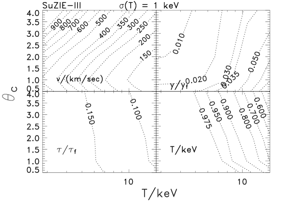
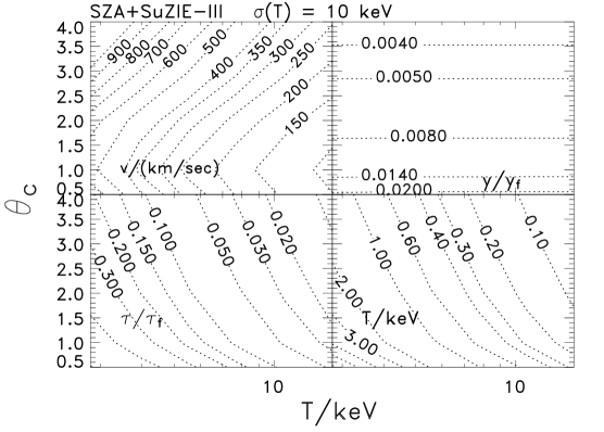
Figure 8.— Forecasted uncertainties for planned experiments as a function of gas temperature and core radius. Left and center are for ACT and a one-hour SuZIE-III observation respectively each with a $\pm$1 keV determination of the temperature from X-ray data. Right is for a combined twelve-hour SZA observation with a one-hour per 48 sq. arcmin SuZIE-III observation.

We saw that for the Reference experiment the loss of the 30 GHz channel increased $\sigma(T)$, as well as $\sigma(v)$ for small $\theta_{c}$. The lack of a low frequency channel can therefore be compensated by an X-ray determination of the temperature. Thus we show forecasts for the ACT survey and SuZIE-III observations both complemented by X-ray temperature determinations of $\pm 1$ keV. The results for the two different experiments are very similar. We assume one hour of integration with SuZIE-III for every 48 sq. arcmin covered. Recall that in order to assure good subtraction of the CMB, we assume a map of linear extent $\theta_{M}=4(2\theta_{c}+\theta_{b})$. We have made no attempt to optimize this observing strategy.

The right-most figure in Figure 8 shows that adding a 30 GHz measurement to the millimeter data can break this degeneracy, as we expect from our previous forecasts for the Reference experiment in Fig. 4. In 1 hour of observation with SuZIE III (per 48 sq. arcmin of map) and a 12-hour SZA observation, the peculiar velocity of a cluster can be measured to 250 km s^-1 even without an X-ray measurement of temperature. A low frequency channel will thus be crucial for obtaining peculiar velocity and gas temperatures at high redshift where $X$-ray brightness is very low.

We also see in Figure 8 a temperature error for our fiducial cluster of $\sim 1.5$ keV (and even smaller for larger $\theta_{c}$). At this accuracy level, one expects to begin to see discrepancies between X-ray temperature measurements which are more sensitive to the hotter, inner regions and SZ temperature measurements which are more sensitive to the cooler, outer regions (Mathiesen & Evrard, 2001). Deeper integrations can slowly improve these measurements as seen from the study of dependence of forecasts for the Reference experiment on observation time.

8. Radio Point Source Contamination

We have assumed that (i) the frequency spectrum of cluster radio sources will be sufficiently steep at high frequencies that measurements at 150 GHz and higher will not be contaminated and (ii) that measurements at 30 GHz will be sufficiently high resolution that point sources can be subtracted at that frequency (this is possible with interferometric experiments such as the SZA). Consequently we have concentrated only on the contamination introduced by dusty galaxies known to be strong submillimeter-wavelength emitters and have excluded radio sources from our analysis. We will now justify this omission.

Clusters often contain radio point sources at mJy levels, as seen from 30 GHz SZ measurements (Reese et al., 2002; LaRoque et al., 2003). It is important to note that radio point sources and submillimeter point sources are not the same objects. The excess of radio sources toward galaxy clusters is most likely due to emission from cluster galaxies themselves (Cooray et al., 1998), whereas the dusty galaxies are typically background sources that are not associated with cluster members. Very little is known about the emission from radio point sources at millimeter wavelengths, but their spectra are expected to steepen due to the energy losses of the most energetic electrons to synchotron emission. This is confirmed to some extent by spectral indices measured between 10-90 GHz for bright sources (Herbig & Readhead, 1992; Sokasian et al., 2001), although there is substantial scatter in the measured index. Sokasian et al. (2001) find a mean index of $-$0.5 between 10 and 90 GHz, while Herbig & Readhead (1992) find a mean index at 40 GHz of $-0.8\pm 0.4$. Measurements by Trushkin (2003) of the spectral indices of the 208 point sources detected by WMAP at 40 GHz (Bennett et al., 2003), suggest a mean of $\beta=-0.1$ at 20 GHz with large scatter, but also show that the spectra of radio sources are often not well-approximated by a simple power law.

Sources of only a few mJy at 30 GHz could easily still have mJy fluxes at 150 GHz if the spectrum does not steepen significantly above 90 GHz. We have used the point source counts from WMAP, DASI, VSA and CBI summarized in Bennett et al. (2003) to determine a best fit model of:

$$\frac{dN}{dS_{\nu}}=\frac{N_{0}}{S_{0}}\left(\frac{S_{\nu}}{S_{0}}\right)^{-2.0}$$ (41)

where $N_{0}=30$ per sq. deg. and $S_{0}=1$ mJy. Our expression gives number counts for mJy sources that are slightly lower than White & Majumdar (2003), but that are consistent with those determined by LaRoque et al. (2002) based on SZ measurements of clusters at 30 GHz. Consequently we expect that the number of sources above 0.1 mJy at 30 GHz is less than one per 4 sq arcmin (roughly the size of a moderate cluster). Repeating our Fisher analysis with radio sources at this level, we find that for all the experimental situations we have considered, the peculiar velocity uncertainty for our canonical source is unaffected, even if a spectral index of $\beta=0.0$ is assumed, and the number counts are 10 times higher than we have assumed.

The spectra of mJy radio sources will soon be much better understood when the SZA and the Array for Microwave Background Anisotropy (AMiBA) start operation at 90 GHz. However, a complete understanding of faint radio sources at mm wavelengths will likely require the sensitivity and resolution of the Atacama Large Millimeter Array (ALMA) .

9. Application of Gas Temperature and Peculiar Velocity Measurements

At roughly the level of 1 keV the distinction between X-ray emission-weighted temperatures and electron-weighted temperatures becomes important (Mathiesen & Evrard, 2001), so a comparison of the two “gas temperatures” could be valuable for studies of the physics of the intra-cluster medium.

Furthermore, the pressure-weighted temperature should be an excellent indicator of cluster mass. This could allow independent calibration of the mass scale for galaxy cluster surveys that use X-ray, optical or SZ selection criteria.

The measurement of peculiar velocities using the kinetic SZ effect has been a goal of SZ measurements for many years. Peculiar velocities at large distances will allow measurements of cosmological parameters and reconstruction of the large scale gravitational potential.

The two-point function of radial peculiar velocities is sensitive mainly to $\Omega_{m}$ and largely insensitive to the dark energy equation-of-state parameter, $w_{x}$ or other cosmological parameters. A linear theory calculation of how well the two-point function can constrain $\Omega_{m}$ gives (Peel & Knox, 2002)

$$\Delta\Omega_{m}=0.04\sqrt{400/N}\frac{\langle v^{2}\rangle+\sigma_{v}^{2}}{\left(500~{}{\rm km~{}s^{-1}}\right)^{2}}.$$ (42)

The SuZIE III and ACT collaborations plan to measure optical redshifts for 400 clusters with masses greater than $3\times 10^{14}M_{\odot}$. Since typical errors for peculiar velocities on these may be 300 km/sec and the velocity rms is about 400 km/sec, these data may be able to achieve $\Delta\Omega_{m}\simeq 0.04$.

However, Equation 42 assumes that the variance in our peculiar velocity measurement errors is perfectly well known. In reality, the statistical properties of the errors will be difficult to know well because of their dependence on the subtraction of the contamination of dusty galaxies. If the assumed error variance is different from the actual error variance by $f\langle v^{2}\rangle$ then there will be a systematic error in $\Omega_{m}$ of

$$\Delta\Omega_{m}=f\left(\frac{\partial\ln{\langle v^{2}\rangle}}{\partial\Omega_{m}}\right)^{-1}\simeq 0.02(f/0.1)$$ (43)

independent of the number of clusters measured. To control this systematic error, we will need to learn more about the spectral properties and luminosity functions of sub-mm galaxies. To avoid this source of systematic error one could use a linear statistic, the average difference between the radial velocities of two clusters separated by distance $r$ (Juszkiewicz et al., 1999). How this statistic depends on cosmological parameters is under investigation.

Another application of peculiar velocities is gravitational potential reconstruction (Dekel et al., 1990). As Dore et al. (2003) point out, due to the low number density of clusters this is only possible on very large scales. Comparison with reconstruction from galaxy number counts can determine galaxy biasing properties. A good understanding of the large scale potential would be valuable for investigating environmental effects on galaxy formation and would be a starting point for constrained realizations of simulations of the large–scale structure of our universe.

10. Discussion and Conclusions

Contamination by emission from dusty galaxies will make accurate measurements of peculiar velocities difficult. With four observing frequencies, few $\mu K$ sensitivity, and arcminute resolution it will be possible to measure peculiar velocities at the level of roughly 200 km/s for massive galaxy clusters.

For comparison, previous estimates of uncertainties in peculiar velocities by Holder (2003) assumed $\mu{\rm K}$ sensitivity and perfect point source removal, which on Figure 4 roughly correspond to $\sigma_{\alpha}=0$ and an observing time of several tens of hours. In that case it was found that uncertainties well below 100 km/s were possible, as could be extrapolated from Figure 4. Such exposure times may be prohibitively long and removing point source contributions to this level will likely require ALMA. ALMA will provide both a better understanding of the physical nature of dusty galaxies in general as well as measurements of the contaminating galaxy fluxes at exactly the frequencies of interest.

The Reference experiment, as well as combinations of planned observations, can provide measurements of peculiar velocities at the level of 150-200 km/s, even in the presence of contamination by dusty galaxies. This is sufficient accuracy to constrain $\Omega_{m}$ to better than 10%. At the same time galaxy cluster temperature measurements will be possible at the keV level. This will allow interesting comparisons with X-ray spectroscopic measures of the X-ray emission-weighted temperature.

Peculiar velocities measured using the kinetic SZ effect, a long-standing challenge to CMB experimentalists, may soon be a reality. The final limiting obstacle appears to be contamination from dusty galaxies, but sensitive multi-frequency measurements should clear this hurdle.

References

- Aghanim et al. (2001) Aghanim, N., Górski, K. M., & Puget, J.-L. 2001, A&A, 374, 1
- Aghanim et al. (2003) Aghanim, N., Hansen, S. H., Pastor, S., & Semikoz, D. V. 2003, Journal of Cosmology and Astro-Particle Physics, 5, 7
- Bennett et al. (2003) Bennett, C. L., Hill, R. S., Hinshaw, G., Nolta, M. R., Odegard, N., Page, L., Spergel, D. N., Weiland, J. L., Wright, E. L., Halpern, M., Jarosik, N., Kogut, A., Limon, M., Meyer, S. S., Tucker, G. S., & Wollack, E. 2003, ApJS, 148, 97
- Benson et al. (2003a) Benson, B. A., Church, S. E., Ade, P. A. R., Bock, J. J., Ganga, K. M., Hinderks, J. R., Mauskopf, P. D., Philhour, B., Runyan, M. C., & Thompson, K. L. 2003a, ApJ, 592, 674
- Benson et al. (2003b) Benson, B. A., Church, S. E., Ade, P. A. R., Bock, J. J., Ganga, K. M., & Thompson, K. L. 2003b, in prep.
- Birkinshaw (1999) Birkinshaw, M. 1999, Physics Reports, 310, 97
- Blain (1998) Blain, A. W. 1998, MNRAS, 297, 502
- Borys et al. (2003) Borys, C., Chapman, S., Halpern, M., & Scott, D. 2003, MNRAS, 344, 385
- Carlstrom et al. (2002) Carlstrom, J. E., , Holder, G. P., & Reese, E. D. 2002, ARA&A, 40, 643
- Challinor & Lasenby (1998) Challinor, A., & Lasenby, A. 1998, ApJ, 499, 1
- Challinor & Lasenby (1999) —. 1999, ApJ, 510, 930
- Cooray et al. (1998) Cooray, A. R., Grego, L., Holzapfel, W. L., Joy, M., & Carlstrom, J. E. 1998, AJ, 115, 1388
- De Grandi & Molendi (2002) De Grandi, S., & Molendi, S. 2002, ApJ, 567, 163
- Dekel et al. (1990) Dekel, A., Bertschinger, E., & Faber, S. M. 1990, ApJ, 364, 349
- Dolgov et al. (2001) Dolgov, A. D., Hansen, S. H., Pastor, S., & Semikoz, D. V. 2001, ApJ, 554, 74
- Dore et al. (2003) Dore, O., Knox, L., & Peel, A. 2003, ApJ, 585, L81
- Dunne et al. (2000) Dunne, L., Eales, S., Edmunds, M., Ivison, R., Alexander, P., & Clements, D. L. 2000, MNRAS, 315, 115
- Dupke & Bregman (2002) Dupke, R. A., & Bregman, J. N. 2002, ApJ, 575, 634
- Fischer & Lange (1993) Fischer, M. L., & Lange, A. E. 1993, ApJ, 419, 433
- Girardi et al. (1996) Girardi, M., Fadda, D., Giuricin, G., Mardirossian, F., Mezzetti, M., & Biviano, A. 1996, ApJ, 457, 61
- Griffin et al. (2002) Griffin, M. J., Bock, J. J., & Gear, W. K. 2002, Appl. Opt., 41, 6543
- Haehnelt & Tegmark (1996) Haehnelt, M. G., & Tegmark, M. 1996, MNRAS, 279, 545
- Hansen (2004) Hansen, S. 2004, MNRAS, submitted, astroph/0401391
- Herbig & Readhead (1992) Herbig, T., & Readhead, A. C. S. 1992, ApJS, 81, 83
- Holder (2003) Holder, G. P. 2003, ApJ, in press, astroph/0207600
- Holder & Carlstrom (2001) Holder, G. P., & Carlstrom, J. E. 2001, ApJ, 558, 515
- Holzapfel et al. (1997) Holzapfel, W. L., Wilbanks, T. M., Ade, P., Church, S. E., Fischer, M., Mauskopf, P., & Lange, A. E. 1997, ApJ, 479, 17
- Hu & Dodelson (2002) Hu, W., & Dodelson, S. 2002, ARA&A, 40, 171
- Itoh et al. (1998) Itoh, N., Kohyama, Y., & Nozawa, S. 1998, ApJ, 502, 7
- Juszkiewicz et al. (1999) Juszkiewicz, R., Springel, V., & Durrer, R. 1999, ApJ, 518, L25
- Lamarre (1986) Lamarre, J. M. 1986, Appl. Opt., 25, 870
- Lange (2002) Lange, A. E. 2002, in NASA/CP-211408:Far-IR, Sub-mm & mm Detector Technology Workshop, ed. J. Wolf, J. Farhoomand, & C. McCreight, in press
- LaRoque et al. (2003) LaRoque, S. J., Joy, M., Carlstrom, J. E., Ebeling, H., Bonamente, M., Dawson, K. S., Edge, A., Holzapfel, W. L., Miller, A. D., Nagai, D., Patel, S. K., & Reese, E. D. 2003, ApJ, 583, 559
- LaRoque et al. (2002) LaRoque, S. J., Reese, E. D., Carlstrom, J. E., Holzapfel, W. L., Joy, M., & Grego, L. 2002, ApJ, submitted, astroph/0204134
- Markevitch et al. (2003) Markevitch, M., Gonzalez, A. H., Clowe, D., Vikhlinin, A., David, L., Forman, W., Jones, C., Murray, S., & Tucker, W. 2003, ApJ, submitted, astroph/0309303
- Mathiesen & Evrard (2001) Mathiesen, B. F., & Evrard, A. E. 2001, ApJ, 546, 100
- McCarthy et al. (2003) McCarthy, I. G., Babul, A., Holder, G. P., & Balogh, M. L. 2003, ApJ, 591, 515
- Molnar & Birkinshaw (1999) Molnar, S. M., & Birkinshaw, M. 1999, ApJ, 523, 78
- Nagai et al. (2003) Nagai, D., Kravtsov, A. V., & Kosowsky, A. 2003, ApJ, 587, 524
- Nozawa et al. (1998) Nozawa, S., Itoh, N., & Kohyama, Y. 1998, ApJ, 507, 530
- Peel & Knox (2002) Peel, A., & Knox, L. 2002, in Sources and detection of dark matter and dark energy in the Universe (DM2002), ed. D. Cline
- Reese et al. (2002) Reese, E. D., Carlstrom, J. E., Joy, M., Mohr, J. J., Grego, L., & Holzapfel, W. L. 2002, ApJ, 581, 53
- Rephaeli (1995) Rephaeli, Y. 1995, ARA&A, 33, 541
- Runyan et al. (2003) Runyan, M. C., Ade, P. A. R., Bhatia, R. S., Bock, J. J., Daub, M. D., Goldstein, J. H., Haynes, C. V., Holzapfel, W. L., Kuo, C. L., Lange, A. E., Leong, J., Lueker, M., Newcomb, M., Peterson, J. B., Ruhl, J., Sirbi, G., Torbet, E., Tucker, C., Turner, A. D., & Woolsey, D. 2003, ApJ, submitted, astroph/0303515
- Sazonov & Sunyaev (1998) Sazonov, S. Y., & Sunyaev, R. A. 1998, ApJ, 508, 1
- Smail et al. (1997) Smail, I., Ivison, R. J., & Blain, A. W. 1997, ApJ, 490, L5
- Smail et al. (2002) Smail, I., Ivison, R. J., Blain, A. W., & Kneib, J.-P. 2002, MNRAS, 331, 495
- Sokasian et al. (2001) Sokasian, A., Gawiser, E., & Smoot, G. F. 2001, ApJ, 562, 88
- Stebbins (1997) Stebbins, A. 1997, preprint, astroph/9709065
- Sunyaev & Zel’dovich (1972) Sunyaev, R. A., & Zel’dovich, Y. B. 1972, Comments Astrophys. Space Phys., 4, 173
- Trushkin (2003) Trushkin, S. 2003, Bull. Special Astrophys. Observatory, 55, 90
- White & Majumdar (2003) White, M., & Majumdar, S. 2003, ApJ, submitted, astroph/0308464