Scientific optimization of a ground-based CMB polarization experiment

Abstract

We investigate the science goals achievable with the upcoming generation of ground-based Cosmic Microwave Background polarization experiments, focusing on one particular experiment, QUaD, a proposed bolometric polarimeter operating from the South Pole. We calculate the optimal sky coverage for this experiment including the effects of foregrounds and gravitational lensing. We find that an E-mode measurement will be sample-limited, while a B-mode measurement will be detector-noise-limited. We conclude that a 300 deg² survey is an optimal compromise for a two-year experiment to measure both E and B-modes, and that a ground-based polarization experiment can make an important contribution to B-mode surveys. QUaD can make a high significance measurement of the acoustic peaks in the E-mode spectrum, over a multipole range of $25<\ell<2500$, and will be able to detect the gravitational lensing signal in the B-mode spectrum. Such an experiment could also directly detect the gravitational wave component of the B-mode spectrum if the amplitude of the signal is close to current upper limits. We also investigate how QUaD can improve constraints on the cosmological parameters. We estimate that combining two years of QUaD data with the four-year WMAP data can improve constraints on $\Omega_{b}h^{2}$, $\Omega_{m}h^{2}$, $h$, $r$ and $n_{s}$ by a factor of two. If the foreground contamination can be reduced, the measurement of $r$ can be improved by up to a factor of six over that obtainable from WMAP alone. These improved accuracies will place strong constraints on the potential of the inflaton field.

1 Introduction

The Cosmic Microwave Background (CMB) has proven to be a powerful cosmological probe. Successive generations of experiments have provided a stringent test for the standard Big Bang paradigm and increasingly sensitive measurements of the temperature power anisotropies have led to tight constraints on many of the fundamental cosmological parameters. However, as well as fluctuations in the CMB temperature field, there are also anisotropies in the linear polarization of the CMB. These polarization fluctuations have recently been detected by the DASI experiment [Kovac et al. 2002] and the correlation between the temperature and polarization has been measured by the Wilkinson Microwave Anisotropy Probe (WMAP) satellite [Kogut et al. 2003]. However, to make full use of the CMB, higher sensitivity high resolution polarized measurements are needed. This is the challenge facing the next generation of CMB experiments.

While it is desirable to observe the CMB temperature field from space, to remove atmospheric noise, this is not as important for polarization experiments since the atmospheric emission is not expected to be linearly polarized [Keating et al. 1998]. Therefore, by integrating deeply on relatively small patches of sky (Jaffe, Kamionkowski & Wang, 2000) it is possible to make a measurement of the polarization anisotropies with a comparable signal-to-noise ratio to a satellite experiment on all but the largest angular scales.

The survey design for a ground-based experiment will depend upon the specific science goals of the experiment. In this paper we investigate observing strategies and sky coverage for the forthcoming generation of ground-based CMB polarization experiments, taking into account foreground issues. We will also show how ground-based polarization measurements can help to tighten constraints on the cosmological model.

To be concrete, we focus on one particular experiment, QUaD (QUEST: Q and U Extra-galactic Sub-millimetre Telescope, and DASI: Degree Angular Scale Interferometer). This is a proposal to install QUEST, a high-resolution bolometric array polarimeter, on the azimuth-elevation mount of the DASI instrument. The experiment plans to begin observing from the South Pole in $2005$ [Church et al. 2003].

The remainder of the paper is set out as follows. In Section 2 we briefly review the physics of the CMB polarization. In Section 3 we present the formalism used in the investigation and in Section 4 we show how we have included the effects of foregrounds. Our cosmological model and definitions are presented in Section 5. In Section 6 we present our results for the survey design, and in Section 7 simulate polarization maps. The expected accuracies and multipole coverage of the power spectra are presented in Section 8, and in Section 9 we present the expected parameters constraints for the QUaD experiment. Our findings are summarized in Section 10. We also include an appendix in which we discuss the sensitivity definitions used in our calculations. We begin with a brief review of CMB polarization.

2 Review of CMB polarization

Detailed reviews of the CMB polarization are given by Zaldarriaga (2003) and Hu & White (1997). In this Section we give a brief overview of how the polarization field is generated and how it is parameterized.

2.1 Parameterization of the polarization field

Typically, a linearly polarized source is quantified by the Q and U Stokes parameters, which give the differences in intensity between orthogonal polarization states. These quantities are convenient to measure experimentally, but are not invariant under a rotation of the co-ordinate system and so are difficult to compare to theoretical models. It is useful to define the quantities $Q(\theta,\phi)\pm iU(\theta,\phi)$ which under rotation acts as a spin 2 quantity. By operating on $Q\pm iU$ using spin raising and lowering operaters it is possible to obtain two rotationally invariant spin 0 fields, $E(\theta,\phi)$ and $B(\theta,\phi)$ (Zaldarriaga & Seljak, 1997). This represents the decompostion of the polarization field into different parity states, the E field is unchanged by a parity transformation, but the B field changes sign. These E and B fields can then be compared directly to theoretical predictions.

The temperature field is usually expanded in terms of scalar spherical harmonics, $Y_{\ell m}(\theta,\phi)$:

$$\frac{\Delta T(\theta,\phi)}{T_{o}}=\sum_{\ell m}T_{\ell m}Y_{\ell m}(\theta,\phi),$$ (1)

where $\Delta T$ is the deviation of the temperature field from its average value $T_{o}$. Similarly, the quantities $Q\pm iU$ can be expanded in terms of spin 2 spherical harmonics, ${}_{\mp 2}Y_{\ell m}$:

$$Q(\theta,\phi)\pm iU(\theta,\phi)=\sum_{\ell m}\left(E_{\ell m}\mp iB_{\ell m}\right)_{\mp 2}Y_{\ell m}(\theta,\phi).$$ (2)

The two point statistics of the CMB can be completely described in terms of the covariances of the multipole moments, $T_{\ell m},E_{\ell m}$ and $B_{\ell m}$:

$$\begin{array}[]{cc}\left<T_{\ell m}^{*}T_{\ell^{\prime}m^{\prime}}\right>=C_{\ell}^{TT}\delta_{\ell\ell^{\prime}}\delta_{mm^{\prime}}&\left<E_{\ell m}^{*}E_{\ell^{\prime}m^{\prime}}\right>=C_{\ell}^{EE}\delta_{\ell\ell^{\prime}}\delta_{mm^{\prime}}\\ \left<B_{\ell m}^{*}B_{\ell^{\prime}m^{\prime}}\right>=C_{\ell}^{BB}\delta_{\ell\ell^{\prime}}\delta_{mm^{\prime}}&\left<T_{\ell m}^{*}E_{\ell^{\prime}m^{\prime}}\right>=C_{\ell}^{TE}\delta_{\ell\ell^{\prime}}\delta_{mm^{\prime}}\\ \left<T_{\ell m}^{*}B_{\ell^{\prime}m^{\prime}}\right>=C_{\ell}^{TB}\delta_{\ell\ell^{\prime}}\delta_{mm^{\prime}}&\left<E_{\ell m}^{*}B_{\ell^{\prime}m^{\prime}}\right>=C_{\ell}^{EB}\delta_{\ell\ell^{\prime}}\delta_{mm^{\prime}}.\par\end{array}$$ (3)

As the B field has opposite parity to the T and E fields the TB and EB correlations are zero if we can assume that parity is conserved. If the CMB is a Gaussian random field, as predicted if the metric fluctuations are generated by zero-point fluctuations during inflation, the statistical properties of the CMB temperature and polarization fields are completely defined by the four power spectra, $C_{\ell}^{TT},C_{\ell}^{EE},C_{\ell}^{BB}$ and $C_{\ell}^{TE}$. However, as we shall discuss in Section 2.3, gravitational lensing by large-scale structure along the line of sight will distort the pattern of fluctuations, and will induce non-Gaussianity.

2.2 Polarization signal generated during recombination

The CMB polarization signal primarily arises from the Thomson scattering of the CMB photons during recombination. Polarization can only be generated if the radiation field contains a local quadrupole. Density perturbations will produce a velocity gradient in the primordial plasma so that photons approaching an electron from different directions will be Doppler shifted by different amounts. This produces local quadrupoles in the radiation field. Before recombination, the high electron density means that the mean free path of the photons is too small to produce a quadrupole; however, after the recombination the electron density is too low for significant Thomson scattering to occur. The polarization can only be produced during a short period around recombination, so the amplitude of the polarization is very low.

The mechanism by which these scalar perturbations are produced in the polarization field is therefore subtly different to the way in which the temperature perturbations are produced. A measurement of the polarization power spectra will not only provide a consistency check of the cosmological model, but will also yield new information on processes occurring in the early universe. Much of this information is contained in the TE and EE acoustic peaks at high $\ell$ which can be measured with high signal to noise with a ground-based experiment.

The inflationary model also predicts a stochastic background of gravitational waves (GW) which will also result in a quadrupole. The decomposition of the polarization field into the E and B modes can be used to separate the GW (tensor) contribution from the density perturbation (scalar) contribution. The E-modes can be produced by both scalar and tensor perturbations, but the B-modes produced at last scattering can only be generated by tensor perturbations. This means that a measurement of the B-mode spectrum would give new information about inflationary parameters. In particular, the amplitude of the tensor spectrum is directly related to the energy scale of inflation. These parameters can not be well constrained from the TT and EE spectrum as it difficult to separate the tensor and scalar contributions to these measurements. The GW B-mode signal peaks around scales of about $\ell=100$ and so in principle is detectable from the ground.

2.3 Polarization signal generated after recombination

The polarization spectra generated at recombination will be altered mainly by two processes before they can be detected: re-ionization and weak gravitational lensing (GL). The effect of re-ionization is to increase the polarization signal on large scales ($\ell\leq 20$). Ground-based experiments are unlikely to be able to measure the polarization on such large angular scales and so will not be sensitive to the effects of re-ionization. However, weak lensing affects the signal on small angular scales. CMB photons are deflected by the gravitational potential of large scale structure. For the TT and EE spectra, this effect results in a smearing of the acoustic peaks on small angular scales, although the change to the spectra is very small, as shown in Fig. 1. However, lensing will also convert E-mode polarization into B-modes. This means that there will be a scalar contribution to the B-mode spectrum due to lensing. Therefore, the B-mode spectrum will be contaminated by a GL contribution, the spectrum of which must be measured precisely so that it can be removed [Knox & Song 2002, Kesden, Cooray & Kamionkowski 2002]. As the lensing signal peaks at small angular scales, ground-based experiments are well-suited to this task.

The lensing signal itself also contains useful information about large-scale structure. This can be used to constrain other cosmological parameters such as the neutrino mass [Kaplinghat, Knox & Song 2003], since this will add to the mass-energy of the universe, altering its expansion history, and suppressing small scale power in the matter power spectrum due to free streaming. The lensing signal will also make the CMB sensitive to the equation of state of the universe, parameterized by $w=p/\rho$, as again this will affect the expansion history.

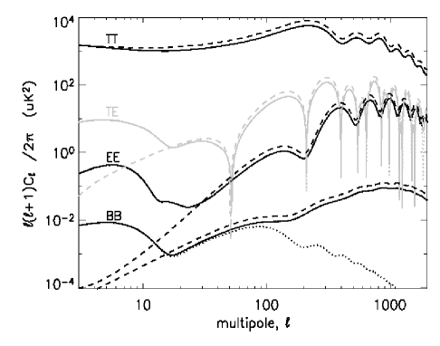
Figure 1: CMB temperature and polarization power spectra. The dashed lines are for a model with no re-ionization while the dotted lines are for a model with no gravitational lensing. The solid lines include the effects of both gravitational lensing and re-ionization. Model parameters are given in Section 5.

Fig. 1 shows the temperature and polarization power spectra, generated by the Boltzmann and Einstein solver CMBFAST (version 4.2; Seljak & Zaldarriaga (1996), decomposed into temperature-temperature (TT) power, temperature-E-mode (TE) cross-power, E-mode-E-mode (EE) power, and B-mode-B-mode (BB) power. We plot spectra without gravitational lensing (dotted lines) and without re-ionization (dashed lines) and with both included (solid lines). The main aim of this paper is to determine the best survey design for the measurement of the polarization spectra. In the following section we present our formalism for this procedure, based on the Fisher Information matrix.

3 Formalism

3.1 Fisher Information matrix

For a model dependent on a set of parameters, $\alpha$, the probability of a particular parameter set, given a set of experimental data points, $\bf{d}$, is expressed by the likelihood function, $L($$\alpha$$\mid\!\!\bf{d})$, the probability of the parameters given the data. By exploring the parameter space to maximize $L$ we may determine the parameter values within certain error limits. The minimum possible variance with which a parameter can be measured can be estimated from the Fisher information matrix [Tegmark, Taylor & Heavens 1997], defined as:

$${\cal F}_{ij}=\left<\frac{\partial^{2}{\cal L}}{\partial\alpha_{i}\partial\alpha_{j}}\right>,$$ (4)

where ${\cal L}=\!-\ln L$ and the derivatives are evaluated at the maximum likelihood values of the parameters. The inverse of the Fisher matrix gives the parameter covariance matrix, ${\cal C}_{ij}$, for the theoretical parameters:

$${\cal C}_{ij}\equiv\langle\Delta\alpha_{i}\Delta\alpha_{j}\rangle={\cal F}_{ij}^{-1},$$ (5)

where $\Delta\alpha_{i}$ is the deviation of the parameter from its maximum likelihood value. The diagonal of the inverse Fisher matrix yields the marginalized 1-$\sigma$ error on the parameters. Taking the inverse of the diagonal of the Fisher matrix,

$$(\Delta\alpha_{i})^{2}=1/{\cal F}_{ii},$$ (6)

yields the conditional error on the parameters. In general

$$[{\cal F}^{-1}]_{ii}\geq 1/{\cal F}_{ii},$$ (7)

where the equality holds only for uncorrelated parameters. The Fisher matrix then provides a theoretical upper bound on the accuracy of a measurement of a given parameter for a given experiment.

3.2 Application of Fisher matrix to CMB experiments

For a CMB experiment, the data are the measurements of the four CMB power spectra and the parameters are the cosmological parameters. For the measurement of a single power spectrum, $C_{\ell}$, the Fisher matrix is given by:

$${\cal F}_{ij}=\sum\limits_{\ell}\frac{1}{(\Delta C_{\ell})^{2}}\frac{\partial C_{\ell}}{\partial\alpha_{i}}\frac{\partial C_{\ell}}{\partial\alpha_{j}},$$ (8)

where

$$(\Delta C_{\ell})^{2}=\frac{2}{(2\ell+1)f_{sky}\Delta\ell}(C_{\ell}+N_{\ell})^{2}$$

is the error in the measurement of the power spectrum in a band centred on multipole $\ell$, and $N_{\ell}$ is a noise term. The survey area is given by $f_{sky}$. The summation is over pass-bands of width $\Delta\ell$.

For a measurement of all four power spectra this generalizes to [Zaldarriaga & Seljak 1997]:

$${\cal F}_{ij}=\sum\limits_{\ell}\sum\limits_{XY}\frac{\partial C_{\ell}^{X}}{\partial\alpha_{i}}\left[\,\mbox{\boldmath$\Xi$}_{\ell}\right]_{XY}^{-1}\frac{\partial C_{\ell}^{Y}}{\partial\alpha_{j}},$$ (9)

where $X$ and $Y$ are either TT, EE, TE or BB and $\Xi_{XY}\equiv{\rm Cov}(C^{X}_{\ell}C^{Y}_{\ell})$ is the power spectra covariance matrix:

$${\mbox{\boldmath$\Xi$}}_{\ell}=\left(\begin{array}[]{cccc}{\Xi}_{\ell}^{TT,TT}&{\Xi}_{\ell}^{TT,EE}&{\Xi}_{\ell}^{TT,TE}&0\\ {\Xi}_{\ell}^{TT,EE}&{\Xi}_{\ell}^{EE,EE}&{\Xi}_{\ell}^{EE,TE}&0\\ {\Xi}_{\ell}^{TT,TE}&{\Xi}_{\ell}^{EE,TE}&{\Xi}_{\ell}^{TE,TE}&0\\ 0&0&0&{\Xi}_{\ell}^{BB,BB}\end{array}\right).$$ (10)

The terms in the power spectra covariance matrix are given by:

$$\Xi_{\ell}^{xy,x^{\prime}y^{\prime}} = \frac{1}{(2\ell+1)f_{sky}\Delta\ell}$$ (11)

$$\times \big{[}(C_{\ell}^{xy^{\prime}}+N_{\ell}^{xy^{\prime}})(C_{\ell}^{yx^{\prime}}+N_{\ell}^{yx^{\prime}})$$

$$+(C_{\ell}^{xx^{\prime}}+N_{\ell}^{xx^{\prime}})(C_{\ell}^{yy^{\prime}}+N_{\ell}^{yy^{\prime}})\big{]},$$

where $(x,y)=(T,E,B)$. The noise covariance is given by $N_{\ell}^{xy}$. In the case of no foregrounds this is given by:

$$N_{\ell}^{xy}=w_{x}^{-1}|{\cal B}_{\ell}^{x}|^{-2}\delta_{xy},$$ (12)

where, $w_{x}^{-1}=\Omega_{pix}^{x}(\sigma_{pix}^{x})^{2}$, for an experiment with solid angle per pixel, $\Omega_{pix}$, and the noise per pixel, $\sigma_{pix}$. The pixel noise depends on survey design and instrument parameters. For an experiment covering an area $\Theta^{2}$ for an integration time $t_{obs}$, with $N_{\rm PSB}$ detectors, a solid angle per pixel $\Omega_{pix}$ and a sensitivity, NET, the pixel noise is:

$$\sigma_{pix}^{2}=\frac{{\rm NET}^{2}\Theta^{2}}{t_{obs}N_{\rm PSB}\Omega_{pix}}.$$ (13)

In Section 4 we discuss how the noise terms may be extended to include foregrounds. We assume that the pixel size used in the map wil be the same as the beam size of the telescope. The spherical harmonic transform of the beam is given by ${\cal B}_{\ell}$. Here we assume that the beam is a Gaussian,

$${\cal B}_{\ell}=\exp\left(-\ell(\ell+1)\sigma_{\cal B}^{2}/2\right),$$ (14)

with $\sigma_{\cal B}=\theta_{\cal B}/\sqrt{8\ln 2}$ where $\theta_{\cal B}$ is the full width half maximum beam size. The pixel size can then be approximated by $\Omega_{pix}=\theta_{\cal B}^{2}$.

The minimum resolution of the power spectra, $\Delta\ell$, depends on the area of sky covered, $\Delta\ell=\pi/\Theta$. This will therefore also give the minimum $\ell$ at which the power spectra can be measured as discussed further in Section 6.2. If a resolution smaller than this is used, the different $\ell$ modes will become correlated and equation (3) will no longer apply [Hobson & Magueijo 1996]. We calculate the maximum $\ell$ value from the FWHM beam size, $\ell_{max}=\pi/\theta$. In reality, multipoles higher than this could be measured if the beam profiles can be accurately determined.

The Fisher matrix also provides a simple way to calculate the results obtainable by combining a number of observations from different CMB experiments. In the simplest case, in which $N_{exp}$ experiments observe different patches of sky, the combined Fisher matrix, ${\cal F}^{C}$, is the sum of the individual Fisher matrices, ${\cal F}^{e}$ [Hu 2001]:

$${\cal F}_{ij}^{C}=\sum\limits_{e=1}\limits^{N_{exp}}{\cal F}_{ij}^{e}.$$ (15)

If any of the patches of sky overlap, each overlapping region is considered as a separate patch. In these patches the combined noise covariance, $N_{\ell}$, of the overlapping experiments should be used to calculate the terms in the power spectra covariance matrix (equation (11)). This is discussed further in the next section where we consider how to optimally combine multi-frequency data.

This completes the formal machinery we will require for our analysis. Note that we have ignored the effects of windowing and mode-mixing due to limited sky coverage (e.g. Bunn 2002), and non-Gaussianity and mode-coupling induced by gravitational lensing (e.g. Guzik, Seljak & Zaldarriaga 1999). The former effects modes by convolving them with the survey window function and mixing $E$ and $B$ modes. This will mainly effect the B-modes, where the signal-to-noise is poor, and will slightly increase our uncertainties. Non-Gaussianity induced by gravitational lensing will also correlate modes and will give rise to higher-order correlations, which will also lead to a slight increase in our uncertainties.

So far we have also ignored the effects of foreground contamination, and it is to this we now turn.

4 Foregrounds

4.1 Including foregrounds into the formalism

The signal measured from the sky will contain not only a component from the CMB, but also a contribution from astrophysical foregrounds. The CMB signal is independent of the wavelength of the observation, but the signal from most foregrounds is expected to be frequency dependent. By observing in a number of different frequency channels it is therefore possible to reduce the total foreground contamination by optimally combining the signal from different frequency channels. It may also be possible to use the multiple frequency information to remove some of the foreground contamination from the signal (e.g. Maino et al. 2002, Hobson et al. 1998).

The effect of observing over multiple channels needs to be taken into account in the Fisher matrix formalism described in the previous Section. If we ignore foregrounds and consider only detector noise, we can simply replace the noise terms in equation (11) by an inverse variance weighting of the noise in each channel, $N_{\ell,c}$:

$$N_{\ell}=\left(\sum_{c}\frac{1}{N_{\ell,c}}\right)^{-1}.$$ (16)

By choosing this weighting scheme at each multipole we combine the signals by giving the most weight to the channels with the smallest detector noise.

We include the effect of foregrounds by treating the foregrounds as an extra source of noise with power spectra $N_{\ell}^{fg}$ for each different power spectra in each frequency channel. This gives us the maximum possible foreground contamination i.e. the contamination assuming that no foreground removal will be attempted. However, unlike the detector noise, the foregrounds will be correlated between power spectra and between frequency channels. To include these correlations we follow the technique developed in Tegmark et al. (2000, hereafter T00). We define a $3F\times 3F$ noise matrix, ${\cal{N}}_{\ell}$, for each multipole, where $F$ is the number of frequency channels in the experiment:

$${\cal{N}}_{\ell}=\left(\begin{array}[]{ccc}{\mathbf{N}}_{\ell}^{TT}&{\mathbf{N}}_{\ell}^{TE}&0\\ {\mathbf{N}}_{\ell}^{TE}&{\mathbf{N}}_{\ell}^{EE}&0\\ 0&0&{\mathbf{N}}_{\ell}^{BB}\end{array}\right),$$ (17)

where each component of this matrix, ${\mathbf{N}}_{\ell}^{XX^{\prime}}$, is an $F\times F$ matrix giving the variances and covariances of the noise in the $F$ channels. Each element in ${\cal{N}}_{\ell}$ is the sum of the contribution from each of the possible foregrounds, ${\mathbf{N}}_{\ell(k)}^{XX^{\prime}}$ and the detector noise, ${\mathbf{N}}_{\ell(det)}^{XX^{\prime}}$:

$${\mathbf{N}}_{\ell}^{XX^{\prime}}={\mathbf{N}}_{\ell(det)}^{XX^{\prime}}+\sum_{k}{\mathbf{N}}_{\ell(k)}^{XX^{\prime}},$$ (18)

where the sum over $k$ is a sum over each of possible foregrounds which could contribute to the signal. We define the $3F\times 3$ scan matrix, $A$, where:

$$\mbox{\boldmath$A$}=\left(\begin{array}[]{ccc}{\mathbf{e}}&0&0\\ 0&{\mathbf{e}}&0\\ 0&0&{\mathbf{e}}\end{array}\right),$$ (19)

and ${\mathbf{e}}$ is a column vector of height F consisting entirely of ones. If $F=2$ as would be the case for QUaD (see Section 6.2) then:

$$\mbox{\boldmath$A$}=\left(\begin{array}[]{ccc}1&0&0\\ 1&0&0\\ 0&1&0\\ 0&1&0\\ 0&0&1\\ 0&0&1\\ \end{array}\right).$$ (20)

The weighted noise for each polarization is then obtained by calculating the $3\times 3$ covariance matrix, $\Sigma_{\ell}$, where:

$$\Sigma_{\ell}=\left(\mbox{\boldmath$A$}^{t}{\cal{N}}_{\ell}\mbox{\boldmath$A$}\right)^{-1}=\left(\begin{array}[]{ccc}N_{\ell}^{TT}&N_{\ell}^{TE}&0\\ N_{\ell}^{TE}&N_{\ell}^{EE}&0\\ 0&0&N_{\ell}^{BB}\end{array}\right).$$ (21)

The terms, $N_{\ell}^{XX}$ are now the noise terms used in equation (11) to calculate the power spectra covariance matrix. If the noise is not correlated between T and E and not correlated between channels (as is the case if we include only detector noise) then ${\cal{N}}_{\ell}$ becomes diagonal and the procedure is identical to the minimum variance weighting of equation (16).

In the last section we discussed how to combine a number of experiments by adding the Fisher matrices of independent patches of sky. For patches in which a number of experiments overlap, the required noise term, $N_{\ell}$, can be calculated by considering a single experiment with channels at each of the different frequencies used by this set of experiments. For this patch $F$ will then become the total number of frequency channels in the combined survey. If any of the instruments used have channels which cannot measure either temperature or polarization, then rows and columns corresponding to these channels should be removed from the full noise matrix, ${\cal{N}}_{\ell}$ and from the scan matrix, $A$, in the relevant places. For example, QUaD would not be able to measure temperature information (see Section 6.2). If we combine the two QUaD channels with another experiment measuring both temperature and polarization, these two channels should be removed from the first row and first column of the matrix ${\cal{N}}_{\ell}$ in equation (17) and the size of the vector ${\mathbf{e}}$ in the first column of the matrix $A$ in equation (19) should be reduced.

4.2 Foreground models

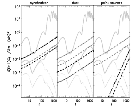
Figure 2: Models used for vibrating dust, synchroton emission and residual point sources (black) compared to the EE and BB power spectra (light grey, solid). The different lines show foreground models at 100 GHz (dash-dot) and 150 GHz (dash). The total foreground power spectra are also shown on each plot (dark grey). The GW component of the BB-spectra is shown for $r=0.1$ (upper dotted line) and $r=0.01$ (lower dotted line). The other foregrounds are either unpolarized or can be neglected

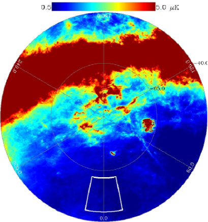
Figure 3: Equal-area zenithal projection showing foreground levels (dust and synchrotron) at 150 GHz in regions which would be accessible to QUaD. The Southern Celestial Pole in located in the centre of the plot, and declination -45 around the perimeter. To the bottom is Right Ascension 0, increasing in RA in the anti-clockwise direction. The possible QUaD observing region is shown by solid lined box.

We closely follow T00 in constructing the foreground power spectra required in the previous section, and use the software provided on the associated website . QUaD proposes to observe at frequencies of 100 and 150 GHz. At these frequencies the relevant foregrounds are diffuse free-free emission, IR and radio point sources, synchrotron radiation and vibrating dust, rotating dust and thermal Sunyaev-Zeldovich (SZ) radiation. Each foreground is modelled using a spatial power spectrum, $C_{l}\left(k\right)=\left(p\cal{A}\right)^{2}l^{-\beta}$, where $\beta$ gives the scale dependence of the foreground fluctuations, $p$ is the fraction polarized and $\cal{A}$ is the overall amplitude. A frequency dependence is also defined and normalized to unity at a reference frequency, $\nu_{*}$. For point sources it is assumed that very bright sources (5 $\sigma$ outlyers) will be removed from the CMB maps, but that there will still be a residual point source contamination after this subtraction. In T00, sets of estimates for these parameters are given. We begin by using their “middle-of-the-road” foreground model. In this model, the only polarized foregrounds are sychrotron, dust and point sources. We then slightly modify this model to take into account recent observations (Kovac et al. 2002; Bennett et al. 2003, hereafter B03). These modifications lower the amplitude of the vibrating dust component and slightly increase the amplitude of the synchrotron emission. The amplitudes then roughly match those given in Fig. 10 of B03. Also following B03 we have lowered the amplitude of the radio point sources and have neglected rotating dust emission. The values of those foreground parameters which are different from T00 are given in Table 1.

Table 1: Parameters used in foreground models which differ from those used in T00. All other parameters used are as per the “middle-of-the-road” model in T00.

Foreground	Radio point	Synchrotron	Vibrating Dust
	sources
$\cal{A}/\mu\rm{K}$	0.66	95	7.5
$\nu_{*}$/GHz	-	20	90

The power spectra of the relevant foreground models are shown in Fig. 2 for the two QUaD frequency bands. The sychrotron radiation dominates the foregrounds at $100$ GHz, whereas at 150 GHz both vibrating dust and sychroton radiation are important. The points sources only contribute at very high multipoles. For most of the multipole range of interest the EE spectrum dominates over the foregrounds. However, for the smaller BB signal the total foreground contamination is larger than the signal of interest.

The analysis described in Section 4.1 gives the residual foreground contamination given that foreground power spectra are well known or can be measured from the experimental data. For QUaD we assume that this is reasonable given that other experiments, e.g. WMAP (B03), ARCHEOPS [Benoit et al. 2003] and the recent Boomerang flight [Montroy et al. 2003], will soon provide polarized maps at CMB frequencies. Recent advances in foreground removal techniques [Baccigalupi 2003] indicate that it may be possible to remove some of the foreground noise from the signal. The residual foreground contamination used here therefore gives an upper limit on that which can be expected in the final cleaned maps, given that our foreground models are accurate.

For a ground-based experiment it will also be possible to select preferentially regions of sky to observe in which the foreground fluctuations are small, and so the foreground noise can be reduced further. Fig. 3 shows the region of sky which would be accessible to QUaD from the South Pole and the estimated levels of foreground contamination across this area from dust [Finkbeiner, Davis & Schlegel 1999] and synchroton [Giardino et al. 2002] using the modified foreground models. A possible observing patch for QUaD is also shown in which the mean foreground amplitude is low. However, a more detailed analysis will be performed to choose the final observing patch with the lowest possible foreground variance across the mutipole range of interest. For these reasons we perform the relevant calculations once using the full-sky foreground models descibed here, and again assuming that the foregrounds are negigible.

We conclude that while our current understand of polarized foregrounds is evolving, the expected level of foreground contamination in the EE power spectrum should not be significant. The GL component of the BB power spectrum should also be detectable if patches of sky with low foreground variance can be targeted or if foreground removal techniques can be successfully implemented. This would also mean that the GW B-mode component should be measureable if the tensor-to-scalar ratio is large.

5 Cosmological model

In order to calculate the terms in the power spectrum covariance matrix and the power spectrum derivative we require a model from which to calculate the CMB power spectra. This model is defined by two sets of parameters: the inflationary parameters which parameterize the initial perturbations causing the fluctuations in the CMB, and the cosmological parameters which determine how these initial perturbations are propagated into the observed CMB power spectra. Given a set of parameters, the CMB power spectra can then be calculated using a Boltzmann and Einstein solver. For this work we have used a slightly modified version of CMBFAST $v4.2$.

The initial scalar perturbations are parameterized by:

$$\Delta_{\cal R}^{2}(k)=\Delta_{\cal R}^{2}(k_{0})\left(\frac{k}{k_{0}}\right)^{n_{s}-1},$$ (22)

where $\Delta_{\cal R}^{2}(k)$ is the power spectra of $\cal{R}$, the curvature perturbation in the comoving gauge, and $n_{s}$ is the slope of the scalar power spectrum. The tensor perturbations are given by:

$$\Delta_{T}^{2}(k)=\Delta_{T}^{2}(k_{0})\left(\frac{k}{k_{0}}\right)^{n_{t}},$$ (23)

where $\Delta_{T}^{2}(k)$ is the power spectra of gravitational waves from inflation and $n_{t}$ is the slope of the gravitational wave power spectrum. The amplitude terms are evaluated at the pivot wave number, $k_{0}=0.05\rm{Mpc}^{-1}$. To parameterize the initial perturbations we use three inflationary parameters: $A$, a constant of order unity which is proportional to the amplitude of the initial scalar perturbations, $n_{s}$, the tilt of the power spectra of the initial scalar perturbations and $r$, the ratio of tensor to scalar perturbations. These are the parameters used in the analysis of the WMAP data [Spergel et al. 2003]. We do not consider here the running of the spectral index, $n_{s}^{\prime}$. The exact relationship between $A$ and $\Delta_{\cal R}^{2}(k_{0})$ is derived in Verde et al (2003; equation (32)). The tensor-to-scalar ratio is defined as:

$$r=\frac{\Delta_{T}^{2}(k_{0})}{\Delta_{\cal R}^{2}(k_{0})}.$$ (24)

Note that a number of different definitions are used in the literature. The most common alternatives are to define $r$ in terms of the Newtonian potential:

$$r_{\psi}=\frac{\Delta_{T}^{2}(k_{0})}{\Delta_{\psi}^{2}(k_{0})},$$ (25)

so that $r_{\psi}\simeq(5/3)^{2}r$, or in terms of the CMB radiation quadrupoles:

$$r_{Q}=\frac{C_{2}^{T}}{C_{2}^{S}}.$$ (26)

The relation between $r$ and $r_{Q}$ depends on the cosmological parameters used in the model [Turner & White 1996].

The cosmological parameters we shall consider are $\{\Omega_{b}h^{2},\Omega_{m}h^{2},h,\tau\}$, where $h$ is the Hubble constant in units of $100\,\rm{km}s^{-1}\rm{Mpc}^{-1}$, $\Omega_{b}$ is the energy density of baryons, $\Omega_{m}$ is the total matter density and $\tau$ is the optical depth to the last scattering surface. Again, these are the parameters chosen for the WMAP data analysis [Verde et al. 2003]. The full set of parameters, and is then:

$$\{\Omega_{b}h^{2},\Omega_{m}h^{2},h,\tau,n_{s},r,A\}=$$

$$\{0.0224,0.135,0.71,0.17,0.93,0.01,0.83\}.$$

The values of these parameters are taken from the best-fit WMAP model [Spergel et al. 2003]. Although we do not include $n_{s}^{\prime}$ in our analysis we note that these best-fit parameters from a model which inculdes a non-zero $n_{s}^{\prime}$. For this parameter set the relation between the r and $r_{Q}$ is approximately $r_{Q}\approx 2.8r$ and $\Delta_{\cal R}^{2}(k_{0})=2.45\times 10^{-9}$. The values of these parameters are taken from the best fit WMAP model [Spergel et al. 2003] except for $r$, which cannot be well constrained by this data set. The current upper limit on $r$ is about $0.36$ [Leach & Liddle 2003]. The lowest possible $r$ which can be detected is of the order of $10^{-4}$ [Knox & Song 2002, Kesden, Cooray & Kamionkowski 2002] due to noise left over from the removal of the gravitational lensing signal from the B-mode spectrum. To reflect this range of possible values we perform the calculations, which have strong dependence on $r$, at two different values, $r=0.01$ and $r=0.1$.

6 Survey design

6.1 Method

The optimization of the survey area for a ground based measurement of the CMB polarization has been addressed previously [Jaffe et al. 2000] in the context of making a detection. We extend this work by considering the criteria for a measurement of the polarization spectra including the effects of gravitational lensing and foregrounds.

The main aim of a polarization experiment is to make measurements of the three polarization power spectra, $C_{\ell}^{TE}$, $C_{\ell}^{EE}$ and $C_{\ell}^{BB}$, with the highest possible precision. The error in the measurement of the power spectra is determined by two conflicting factors. For a fixed total observing time, the integration time per unit area (or pixel) is inversely proportional to the total area; a smaller map will therefore result in a lower pixel noise. However, for a smaller map there are fewer independent modes from which to measure each multipole (i.e. the averaging in equation (3) will be made over fewer values of $m$) and so the sample variance will increase.

To quantify these effects, we choose a single parameter for which to evaluate the Fisher matrix, $A^{\!X}$, the amplitude of each power spectrum. For a single parameter the variance in the measurement of this parameter, $(\Delta A^{\!X})^{2}$, is then given by $1/F_{A^{X}\!A^{X}}$. From equation (8) the error in $A^{\!X}$ is:

$$(\Delta A^{\!X})^{2}=\left(\sum\limits_{\ell}\frac{1}{(\Delta C_{\ell}^{X})^{2}}\frac{(C_{\ell}^{X})^{2}}{(A^{\!X})^{2}}\right)^{-1},$$ (27)

where $(\Delta C_{\ell}^{X})^{2}$ for each power spectrum are given by the diagonal elements of the power spectrum covariance matrix in equation (10). We then define a figure of merit parameter as the signal to noise ratio in the measurement of each power spectrum, SNR, which is given by:

$$\rm{SNR}=\left(\frac{A^{\!X}}{\Delta A^{\!X}}\right)=\sqrt{\sum_{\ell}\left(\frac{C_{\ell}^{X}}{\Delta C_{\ell}^{X}}\right)^{2}}.$$ (28)

To find the optimal area for a measurement of each power spectrum with a specfic experiment we therefore need to find the area which gives the highest SNR given a set of survey and instrument parameters.

This optimization procedure could be done for any cosmological parameter, or combination of parameters. However for simplicity, and as a prerequisite to the measurement of the polarization power spectra, we will maximize the SNR for the amplitude. In principle, other parameters for the survey or telescope could be left free, such as the pixels size or beam width. In practice we find that the smallest pixel/beam size is preferred, and so we set this to the limit of a given experiment.

6.2 QUaD instrument parameters

As a specific example of a ground-based experiment we use the QUaD experiment. This enables us to fix the instrument parameters needed to determine the pixel noise (equation 13) and the allowed multipole range. These parameters are given in Table 2. A detailed description of QUaD is given in Church et al. (2003).

The maximum multipole which can be covered is limited by the beamsize as discussed in Section 3. If no other effect needs to be taken into consideration the minimum multipole, $\ell_{min}$, would be determined from the survey area, $\ell_{min}=\pi/\Theta$. However, for a ground-based experiment the lower-$\ell$ cut-off is also limited by the stability of the atmosphere. This will limit the maximum scan which can be used and hence the largest angle on the sky over which a correlation can be made. For a perfect polarization experiment, this would not be an issue, as the unpolarized atmospheric fluctuaions would not be detected in the polarized data. However, instrumental effects will cause a fraction of the unpolarized (common mode) signal to be to be present in the polarized signal. The atmosphere at the South Pole is exceptionally stable [Lay & Halverson 1998] and the QUaD instrument has been designed is such a way that these effects will be minimized, so we estimate that a minimum $\ell$ of $25$ can be reached. The minimum $\ell$ used in equation (28) will then be $\ell_{min}={\rm max}(\pi/\Theta,25)$. Although it is possible for QUaD to make total power measurements, there is no mechanism for removing the atmospheric noise from the resulting data and so we assume that QUaD would not be able to produce temperature maps.

We estimate the total observing time by assuming that QUaD will observe at the South Pole for two years during the austral winter (six months per year) for 22 hours each day and assuming that $20$ per cent of this total time will be lost due to bad weather, instrument maintenance and calibration time. These estimates are based on the experiences of the DASI team at the South Pole site [Kovac et al. 2002]. This gives a total time spent observing on the CMB of $3210$ hours per year. The maximum useable patch of sky is about $1000$ deg², limited by available sky visible from the survey site, and major foreground contamination from the Galactic plane (see Fig. 3). We therefore restrict the analysis to areas below this maximum survey size.

It is important to note that to measure both the Q and U Stokes parameters, each pixel must be measured with the detector in at least two different orientations with respect to the sky. For QUaD this will be achieved by rotating a half-wave plate so that both Q and U can be measured by each detector. This halves the total integration time available for each Stokes parameter when making a polarized measurement.

Table 2: Expected QUaD instrument parameters

Frequency (GHz)	100	150
Number of bolometers	24	38
Angular resolution (arcmin)	6.3	4.2
NET per bolomete$\mbox{r}^{a}$ ($\mu\mbox{K}s^{1/2}$)	270	300

a - The definition of sensitvity for a polarization sensitive bolometer is discussed in Appendix A.

6.3 Results

We have applied the above procedure to a model QUaD experiment. We consider three different cases:

1. a measurement of the EE spectrum,

2. a measurement of the BB spectrum including the lensing component as part of the signal we wish to measure,

3. a measurement of just the BB GW spectrum including the lensing signal as an extra source of noise.

The results for the QUaD parameters are presented in Table 3, for TE, EE and BB spectra, for the case of foregrounds, and without foregrounds. The latter is of interest if the foregrounds are well enough understood to be subtracted from the signal or if a patch of sky with very low foreground variance can be found, as discussed in Section 4

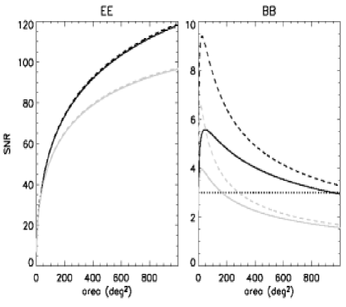
Figure 4: Variation of SNR with survey area for the EE (left) and total BB (right) power spectra with foregrounds (solid lines) and without foregrounds (dashed lines) for an observing time of 1 year (light) and 2 years (dark) for r=0.01

Fig. 4 shows how the SNR varies with area for EE and BB spectra. From Fig. 4 (left) it can be seen that a ground-based polarization experiment can make a good measurement of the EE spectrum, even if the foreground contamination is not well understood. The SNR is close to 100 for survey areas over $300$ deg². Below this size the SNR falls rapidly to zero. For an experiment with the sensitivity and multipole coverage of QUaD, an E-mode survey is sample-variance-limited, so that a larger area is preferable ($>1000$ $\rm{deg}^{2}$) for statistical purposes. Given that an E-survey will have high signal-to-noise per pixel, a high-resolution polarization map of the surveyed area is also possible (see Section 7), allowing for removal of point sources as discussed in Section 4.

Fig. 4 (right) shows the SNR for a two-year B-mode survey. The dotted line is for a SNR=3 which is the minimum SNR that can be considered as an actual detection of the signal. Unlike the E-mode survey, the B-mode survey is detector noise limited as the signal is much lower. With foregrounds the SNR sharply peaks at ${\rm SNR}\approx 5.5$ for much smaller areas, around $50$ deg², where the lensing signal dominates. As the survey area increases the noise per pixel increases and the overall SNR drops. If we can remove foreground contamination then the maximum SNR increases to a value of 9 and the optimal area is slightly reduced, as shown in Table 3.

This different behaviour between the E and B-mode surveys with increasing area makes the simultaneous optimization of both measurements difficult. One compromise is to use the break in SNR of the E-mode survey at around 300 $\rm{deg}^{2}$. Although this is sub-optimal for both surveys, the drop to ${\rm SNR}=90$ for the E-survey is minimal and ${\rm SNR}=4.5$ for the B-mode survey is still a strong detection. An alternative would be to split the survey in two, one large, one small, halving the integration time for each survey. As shown in Fig. 4 for a single year of integration it is still possible to detect the B-mode signal if we concentrate on a small area of sky ($\sim 20$ $\rm{deg}^{2}$). For a single year the EE SNR also does not drop significantly if an area larger than about 500 $\rm{deg}^{2}$ is chosen.

From Table 3 it is evident that QUaD cannot detect the GW B-mode component unless the tensor to scalar ratio is larger than the values considered so far. We have therefore extended the calculation to higher values of $r$ up to the current upper limit. Fig. 5 shows how the optimal area for a measurement of the GW signal with QUaD varies with $r$. The optimal area changes significantly as $r$ increases. For the foreground model assumed here it is only possible to detect the GW signal for $r$ greater than 0.35. However, for the large areas which are best for detecting this high GW signal, the SNR for the total B-mode signal drops significantly. It is therefore not possible to pursue both science goals simultaneously. However, if the foreground comtamination can be completely removed, the lowest detectable value of $r$ drops to 0.14. The optimal area also decreases as the detector noise becomes the dominant factor. In the no foreground case it would be possible to detect the GW signal using the $300$ $\rm{deg}^{2}$ survey discussed above. If the GL signal can be removed, the GW signal becomes slightly easier to detect, but only if the foregrounds can be subtracted as the combined dust and synchroton contamination (Fig. 2) is larger than the GL signal over most of the multipole range which can be covered from the ground.

The effects of the mixing of E and B modes due to partial sky coverage will not significantly influence the results found here. Bunn (2002) finds that the mixing will only have a large effect for the B-mode signal on the scale of the survey size. If we use a $300$ $\rm{deg}^{2}$ patch the GL B-mode signal will therefore not be affected. For a detection of the GW signal this effect will become more important. However, Lewis, Challinor & Turok (2002) discuss this problem and calculate the minimum detectable $r$ as a function of survey size. They find that for the large surveys (greater than $50^{\circ}$) the minimum value is not changed if the mixing effects are included. For the areas discussed here the GW results will therefore not be influenced by E-B mixing if an optimal method is used to separate the E and B modes.

Figure 5: Variation of the survey optimal area (upper plot) and achievable SNR (lower plot) for a measurement of the GW signal with QUaD as a function of $r$ with (solid line) and without (dashed line) foregrounds.

Table 3: SNRs for the optimal survey areas for each of the power spectra for a two-year integration time with QUaD

Spectrum	TE	EE	BB		$GW$
$r$	0.01	0.01	0.01	0.1	0.01	0.1
areaa /$\rm{deg}^{2}$	1000+	1000+	46	50	813	1000+
areab /$\rm{deg}^{2}$	1000+	1000+	24	26	126	247
SNRa	31	118	5.6	5.7	0.1	1.0
SNRb	31	119	9	9	0.4	2.5

a - including astrophysical foregrounds
b - without astrophysical foregrounds

To estimate the SNR for the TE spectrum we assume that a QUaD map could be combined with the portion of the expected four-year WMAP data covering the same area of sky. The results are shown in Table 3. As with the EE spectrum, the measurement is sample-variance-limited and the largest possible area of $1000$ deg² is best. The SNR also drops sharply if the survey area becomes too small ($\leq$ $100$ deg²). However, the QUaD TE measurement is limited by the resolution and sensitivity of the WMAP map and suffers more heavily from sample variance than the smaller EE signal. The SNR with which this spectrum could be measured by QUaD is therefore smaller than the EE SNR. The TE spectrum has also already been measured in this multipole range by WMAP. It is therefore more useful to optimize a ground-based survey for a measurement of the EE and BB spectra.

We have also investigated the effect of increasing the minimum $\ell$ value used in the calculation. For the TE, EE and total BB spectra, an increase in the minimum $\ell$ from 25 to 100 has a negligible effect, as most of the power in these spectra is from the higher multipoles. However, as would be expected, increasing the minimum $\ell$ does affect the GW B-mode detection. If the minimum $\ell$ is increased to 100 the GW is no longer detectable below the current upper limit of $0.36$.

7 Deep maps of the CMB polarization

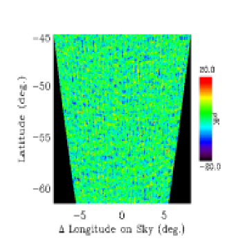
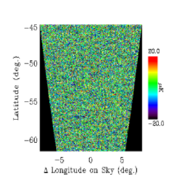
Figure 6: Simulated polarization maps from QUaD (left) and Planck (right), showing a $300$ $\rm{deg}^{2}$ field of Q-mode anisotropies at 150 GHz. All of the structure in the high signal-to-noise QUaD map is real signal, while the Planck map (shown with the same pixelization) has much lower signal-to-noise per pixel. Foregrounds and other systematic effects are not included in either map.

For a ground-based experiment it is not possible to make observations of the whole sky due to the limited sky coverage available from the ground. Although this is a disadvantage in terms of multipole coverage at low $\ell$, by making a deep integration of a small region of sky it is possible to make maps with a very high signal-to-noise ratio. This allows more precise measurements to be made on small angular scales. It will also improve the ability of the experiment to remove low-lying systematic effects which would not be detectable in observations of lower signal-to-noise. We illustrate the difference between QUaD and the Planck satelllite mission in Fig. 6 using simple simulations of the Q Stokes parameter with noise appropriate to each experiment. While Planck will cover much more sky than QUaD, the QUaD observations would be at higher signal-to-noise than the average of those made by Planck. This will allow QUaD to limit systematic effects in the experiment to an unprecented level. This makes the QUaD approach highly complementary to that of Planck, which would have lower average sensitivity, but good statistics over the entire sky. The deep maps will also provide new information on the techology used by QUaD and on polarized foregrounds, which will be crucial for the design of future CMB experiments.

Using a smaller region of sky is also an advantage in terms of foregrounds, as it is possible to target the most useful patches of sky, without spending valuable integration time on regions which will ultimately be left unused in cosmological analyses.

Finally, it is possible tailor the size of the region observed to optimize for a particular science goal. As was described in Section 6, this is especially important for searches for the faint B-mode signal.

8 Power spectra estimation

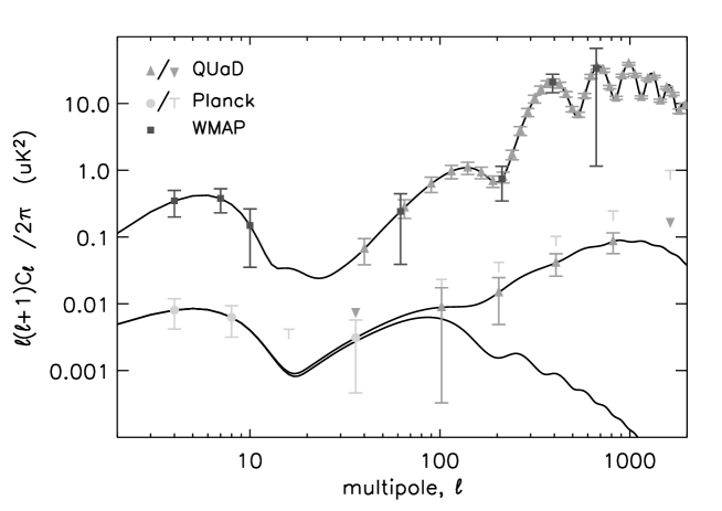
Figure 7: Predicted measurements of the polarization power spectra achievable with the current generation of satellite (four-year WMAP and two-year Planck) and ground-based (two-year QUaD) experiments for $r=0.1$. The error bars show detections above the one-sigma level and the free symbols show upper limits. The errors include a contribution from astrophysical foregrounds. For clarity we do not show the Planck measurements of the EE power spectrum. These will be of a similar sensitivity to the QUaD measurements, but will cover different $\ell$ ranges, as indicated by the points on the B-mode spectrum.

Table 4: Planck and WMAP instrument parameters. For WMAP we use only the highest two frequency channels as the other channels are used mainly to constrain foreground contributions.

	Planck				WMAP
frequency /GHz	40	70	150	220	70	90
NET /$\mu Ks^{1/2}$	220	300	80	120	1521	2071
Beam size /arcmin	24	14	7	5	20	13
Detector number	6	12	8	8	8	16

By statistically averaging over the polarization signal, the polarization power spectra may be estimated. Fig. 7 compares the expected band-averaged power spectra results and multipole coverage of a 300 deg², two-year ground-based experiment, QUaD, an all-sky four-year satellite, WMAP, and the Planck satellite mission. These predictions are based on equation (11), with the parameter the power in a pass-band of width $\Delta\ell$. We include all of the power covariances and effects of foreground emission outlined in Section 4. The instrument parameters used in each experiment are given in Tables 2 and 4.

From this analysis we find that QUaD can make a high-significance measurement of the EE-power spectrum, as suggested by the high SNR ($\sim 90$) found during optimization in Section 6, over a multipole range from $\ell=25$ to $\ell=2500$. The polarization acoustic oscillations are well sampled, with a resolution of $\Delta\ell\approx 20$. The lower modes are not sampled due to the limited survey area. In particular the re-ionization peak at $\ell=7$ is only detected by a satellite mission.

In addition there is a good detection of the BB-power spectrum from $\ell=25$ to $\ell=1000$. Power is binned logarithmically to increase the signal-to-noise per bin. The most significant bin is at $\ell=1000$, at the peak of the gravitational lensing (GL) contribution to the BB-spectrum. If the foreground contamination can be significantly reduced, a direct detection of the GW contribution to the B-mode power spectrum could be made at around $\ell=100$. Again the low-$\ell$ modes are not accessible to a ground-based survey, but can be complementarily detected by an all-sky satellite mission.

With both temperature and polarization data available the TE-cross power spectra may also be estimated so that a cross-check can be made with other measurements of this signal.

With such high-resolution polarization information available it is interesting to see what effect a ground-based survey will have on cosmological parameters.

9 Parameter Estimation

In this Section we investigate the contribution which can be made by ground-based polarization experiments to the measurement of the cosmological parameters. Previous work on CMB parameter estimation (Efstathiou & Bond 1999; Zaldarriaga, Spergel & Seljak 1997; Bond, Efstathiou & Tegmark 1997) has shown that the polarization data which can by obtained by the forthcoming WMAP and Planck satellite missions will allow a more accurate determination of many of the key cosmological parameters. For a satellite experiment, this is mainly because the degeneracy between $\tau$ and $A$ can be broken by measuring the re-ionization bump in the polarization power spectra. These re-ionization bumps also create a high GW B-mode signal at low $\ell$, so a full-sky measurement will also tighten constraints on the tensor-to-scalar ratio.

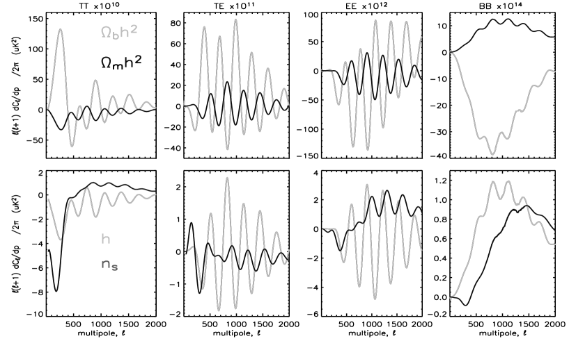
Figure 8: The derivative of the CMB polarization power spectra with the parameters $\Omega_{B}h^{2}$, $\Omega_{m}h^{2}$, $h$, and $n_{s}$. The models are generated by CMBfast, with fiducial parameters given in the text.

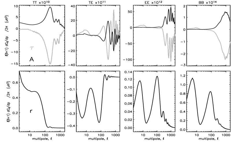
Figure 9: The derivative of the CMB polarization power spectra with the parameters $\tau$, $A$ and $r$. The models are generated by CMBfast, with fiducial parameters given in the text. Note that the plot is now logarithmic in order that the low $\ell$ degeneracy breaking between $\tau$ and $A$ can be observed in the polarization power spectra.

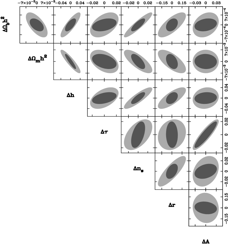
Figure 10: Marginalized Fisher matrix relative parameter error constraints ($\Delta\ln L=-1/2$) anticipated for four-year WMAP results only (dark) and four-year WMAP combined with QUaD (light) for $r=0.01$ with foregrounds. The projections of the ellipse onto the two axes give the standard errors on each parameter. For a two-parameter $68$ per cent confidence region, the ellipses should be scaled by a factor 1.5.

As we have discussed, a ground-based polarization experiment can concentrate on smaller areas of sky at higher resolution and so can make a good measurement of the acoustic peaks out to high $\ell$ in the EE-power spectrum. The information from a ground-based experiment will therefore complement the full-sky satellite data. It is also possible to choose an observing strategy with targets the GW signal peak at intermediate scales ($\ell=100$). Ground-based constraints on the B-mode GW signal will therefore also complement those obtainable from the current generation of satellite experiments.

Finally, it is important to note that a CMB polarization experiment is not just adding more data. A similar experiment measuring only the temperature spectrum, over the same multipole range, and with the same detector sensitivity, would add very little new information as far as cosmological parameters are concerned, although a high-$\ell$ temperature surveys may well start to probe higher-order CMB effects. Hence polarization adds unique information from the CMB.

We investigate the potential increase in the precision of the measurement of cosmological parameters which can be achieved with a ground-based experiment by comparing the expected four-year results from WMAP alone to those which could be achieved by combining QUaD and WMAP data. To compare the two cases we calculate the inverse Fisher matrix using equation (9) to find the variances and covariances between each of the parameters. For QUaD we use the instrument model dicussed in Section 6.2. The experimental parameters used for WMAP are given in Table 4.

To calculate the derivatives in parameter space required in equation (9) we use second-order differencing between CMBFAST models for accuracy, with the corresponding parameter changed up and down by 1 per cent. The derivative of the power spectrum encapsulates the response of the spectrum to a change in a particular parameter and hence quantifies its information content. However, if the shape of the derivative for any two parameters is too similar then the two parameters will be degenerate and cannot both be constrained. The derivatives used in the calculation are shown in Fig. 8 and 9. For most parameters, the shape of the derivatives reflects the acoustic peaks in the power spectrum, indicating that both information about parameters and their differences are contained in the peaks. For instance with temperature only $\Omega_{m}h^{2}$ and $\Omega_{B}h^{2}$ are quite anti-correlated, but their derivatives oscillate out of phase for TE and EE-spectra, breaking this degeneracy. Much of the difference between $h$ and $n_{s}$ occurs in the low multipoles, but there is a large difference at high-$\ell$ in the BB-spectra due to the effects of gravitational lensing on these modes.

Fig. 9 clearly shows the anti-correlation that arises between $\tau$ and $A$ when only temperature information is available. This degeneracy is seen to be broken on large scales by the differences in the responses of the polarization power spectra. However, going to high $\ell$ in the polarization spectra, these parameters become strongly degenerate again. Hence we can expect that a ground-based polarization survey, which will have difficulty reaching the lower multipole range, will not contribute much to lifting the $A-\tau$ degeneracy. Conversely, with only temperature information, $h$ and $n_{s}$ are strongly degenerate, with much of the difference in response coming at very low modes, or modes beyond a few hundred. However, adding polarization information, especially TE at around $\ell$ of 100, and lensed BB modes at high $\ell$, breaks this degeneracy due to their different responses

Finally with only a temperature spectrum, the response to $r$ is limited to the first hundred multipoles. The $TE$ and $EE$ derivatives show that there is useful information about $r$ on intermediate scales in the polarization spectra up to around $\ell=500$, but for these multipoles the scalar EE and TE power spectra are very high and so it will be difficult to extract this information from the signal. However, the BB derivative also shows structure at higher multipoles and will provide information on $r$ if the tensor signal is higher than the scalar lensing signal at the scales of interest, or if the lensing signal can be removed.

Having considered the responses of the power spectra to our parameter set, we now turn to estimating parameter uncertainties from satellite and ground-based surveys. To test the validity of this procedure we have calculated the accuracy achievable with the one-year WMAP data, and found that our results are on good agreement with the one-year WMAP quoted parameter errors [Spergel et al. 2003].

Fig. 10 shows the relative error ellipses (defined by the $\Delta\ln L=-1/2$ contour) expected from a 4-year WMAP experiment (darker ellipses) and from a combined 2-year ground-based QUaD and 4-year WMAP experiment (lighter ellipses) for our fiducial 7-parameter model, marginalizing over the other parameters. The projection of this contour gives the marginalized one-parameter, $1-\sigma$ error for each parameter. For a two-parameter $68$ per cent confidence region, the ellispes should be scaled by a factor 1.5. We assume that the TE-cross spectrum can be estimated in the overlap region. Here we see that a significant improvement of around a factor 2 is made on most of the parameter set by adding in a ground-based polarization survey, despite the significant difference in survey size. For most parameters, this comes from the high-multipole information in the EE-spectra, but there is also important information in the BB-spectra, in particular for $r$, $h$ and $n_{s}$.

The 1-$\sigma$ marginalized parameter uncertainties for WMAP and QUaD + WMAP are shown in Table 5. By including QUaD the precision with which the parameters can be measured is improved by around a factor of two in most cases. This increase in accuracy arises from the extra information in the EE-spectra from modes $\ell\geq 100$, and from the strong BB-spectral dependence on small scales for $n_{s}$ and $h$. Again, for a temperature survey alone Fig. 8 and 9 indicate there is no useful information at high-multipoles.

It is interesting to look at how the information from the B-mode spectrum influences the parameter estimation. To examine this the same calcuation was made, but with the B-mode information removed from the Fisher matrix. For WMAP, this did not change the parameter estimates significantly, except for a slight increase in the error on $r$ ($\sim 10$ per cent). For WMAP most of the information on $r$ must therefore come from the TT, TE and EE spectra, and not from the weak upper limit on the B-mode spectrum. For QUaD we find a slight increase in the errors on $h$ and $n_{s}$ ($\sim 20$ per cent) due to the loss of the information contained in the B-mode lensing signal. However, the error on $r$ more than doubles if B-modes are not included. The B-mode information from QUaD must therefore make a significant contribution to the $r$ constraint, even though QUaD cannot make a strong detection of the GW B-mode signal.

Fig. 11 shows the predicted improvement on a joint measurement of $r$ and $n_{s}$ from a two-year QUaD experiment and four-year WMAP survey. With a detection of $r$, $n_{s}$ and the amplitude $A$, the shape of the inflaton potential can be inferred [Hoffman & Turner 2001].

The poorest parameter improvement is for $\tau$ and $A$, which only improve by a factor of about $1.3$. As discussed above this is because the main differences appear on scales of $\ell\leq 100$, which are difficult to reach from the ground, but accessible to satellite surveys.

We find that for most parameters the errors do not decrease significantly if the foreground contamination is completely removed. However, this is not the case for $r$, where the error decreases by a factor of three if the foreground contamination can be removed, leading to a factor of six improvement over the WMAP-only constraints. This can be clearly seen from the inner contours in Fig. 11. This is because the foreground removal allows a much better measurement of the B-mode GW signal to be made.

Table 5: Fisher matrix estimates of parameter errors

Parameter	Value	WMAP	WMAP +QUaD
$\Omega_{b}h^{2}$	0.0224	0.0009	0.0004
$\Omega_{m}h^{2}$	0.135	0.007	0.004
$h$	0.71	0.040	0.021
$\tau$	0.17	0.023	0.020
$n_{s}$	0.93	0.029	0.014
$r$	0.01 (0.1)	0.206 (0.203)	0.082 (0.090)
$A$	0.83	0.036	0.031

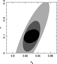
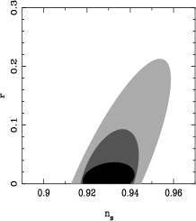
Figure 11: Predicted improvment on a joint measurement of $r$ and $n_{s}$ for two-year WMAP data (outer contour), two-year QUaD + WMAP including foregrounds (middle contour) and two-year QUaD + WMAP without foregrounds (centre contour) for $r=0.1$ (left) and $r=0.01$ (right). The $\Delta\ln L=-1/2$ contour is shown. For 68 per cent confidence limits, scale by a factor 1.5

10 Summary

In this paper we have investigated the science goals achievable with the forthcoming generation of ground-based CMB polarization experiments. We have set out a Fisher information matrix formalism that takes into account the combination of different temperature and polarization surveys, and includes foreground contamination. We have argued that ground-based polarization experiments can reach the high sensitivities required by making a deep integration on a small patch of sky. By preferentially selecting regions of sky with low foreground variance it will also be possible for a ground-based experiment to reduce further the foreground contamination.

Taking the proposed QUaD South Pole experiment as our model survey, we have optimized the survey area and shown that a 300 $\rm{deg}^{2}$ survey is a good compromise between a sample-limited E-mode survey and a detector-noise limited B-mode survey. Below 300 $\rm{deg}^{2}$ the SNR for the E-mode survey drops rapidly, while above this a detection of the (gravitational lensing component of the) BB-power spectrum becomes unfeasable. With such high signal-to-noise per pixel in the E-mode survey, deep imaging maps of the CMB polarization field can be made. Statistically averaging the data allows a high-significance measurement of the EE-power spectrum over a range of multipoles from $\ell=25$ to $\ell=2500$, with good sampling of the acoustic oscillations. The gravitational lensed component of the BB-power spectrum can also be detected with good signal-to-noise. If it is possible to reduce the foreground contamination the gravitational wave could also be detected for $r\geq 0.14$.

Combining a two-year QUaD experiment with a four-year WMAP all-sky survey allows a better measurement of cosmological parameters to be made compared to that possible from WMAP data alone. Most parameters can be improved by a factor two. If the foreground contamination can be reduced the tensor-to-scalar ratio will be dramatically improved by up to a factor of six. With such improvements, strong constraints can be placed on the potential of the inflaton field. Only the degeneracy between the amplitude of fluctuations, $A$, and the optical depth to re-ionization, $\tau$, are not significantly improved, as this requires large scales only accessible to a satellite.

In conclusion we find that if the necessary sensitivity and control of systematics can be achieved, a ground-based CMB polarization experiment such as QUaD can make a major contribution to the study of CMB polarization power spectra and cosmological parameters.

Appendix A Sensitivity definitions for CMB polarization experiments

There are a number of definitions for the sensitivity of a CMB polarization experiment and this is often a cause of confusion when comparing different sensitivity parameters. For a total- power CMB experiment the sensitivity is usually defined in terms of the noise equivalent temperature (NET). This is the signal needed from the source to give a signal-to-noise ratio of unity in a one-second integration time. To measure polarization an equivalent definition is required in terms of the Q and U Stokes parameters. For a linearly polarized source of total intensity, $I$, of which a fraction $p$ is polarized at an angle $\chi$ to the reference direction, the Stokes parameters can be defined as:

$$Q=pI\cos(2\chi),$$

$$U=pI\sin(2\chi).$$ (30)

If we orientate the axis of the reference system so that it is aligned with the polarization angle of the source ($\chi=0$) then we have $U=0$ and $Q=pI$ so that $Q$ gives the total polarized intensity. We can then define the polarization sensitivity, NEQ, as the polarized signal from the source needed to give a signal-to-noise ratio of unity in a one-second integration time for a source with a polarization angle aligned with the reference direction of the measurement.

For QUaD, the polarized measurements will be made with pairs of polarization-sensitive bolometers (PSBs). The two bolometers in a PSB pair are sensitive to orthogonal polarization states of the incoming radiation. The intensity measured by the co-polar ($x$) and cross-polar ($y$) device is given by [Jones et al. 2003]:

$$I_{x}=\frac{1}{2}(I+Q),$$

$$I_{y}=\frac{1}{2}(I-Q),$$ (31)

in a reference system aligned with the polarization angle of the source. The total intensity is found by adding the two bolometer outputs and the $Q$ Stokes parameter is found by differencing the outputs.

For a bolometer, the noise equivalent power due to photon noise (NEP) is given by [Lamarre 1986]:

$$NEP^{2}=2h\nu P+\frac{2P^{2}}{m\Delta\nu}$$ (32)

where is $m$ is the number of polarization states detected ($m$ is either 1 or 2). For a single PSB, $m=1$, as only a single polarization state is detected. $P$ is the power in a band of width $\Delta\nu$:

$$P_{\nu}=\eta_{d}\eta_{t}\varepsilon A\Omega B_{\nu}\Delta\nu,$$ (33)

where $A\Omega$ is the throughput of the system, $\varepsilon$ is the emissivity of the source and $B_{\nu}$ is the intensity of the radiation that would be emitted from a perfect black body. The total efficiency of the system is $\eta=\eta_{d}\eta_{t}$, where $\eta_{d}$ is the detector efficiency and $\eta_{t}$ is the instrument efficiency. We assume that a lossless PSB will absorb half of the incident unpolarized radiation, giving $\eta_{d}=1/2$. The NET due to photon noise in each PSB from the unpolarized background radiation is therefore:

$$NET_{s}=\frac{(2h\nu P+2P^{2}/\Delta\nu)^{1/2}}{\eta_{d}\eta_{t}\>\>\partial B_{\nu}/\partial T},$$ (34)

where the factor of $\eta_{d}\eta_{t}$ is needed to convert from the noise at the detector to the signal required at the source, as only a fraction of the radation from the source will be absorbed by the PSB. $\partial B_{\nu}/\partial T$ is the derivative of the source intensity with respect to temperature and converts from an NEP to an NET. Equation (34) gives the NET for a measurement of the temperature of the CMB with a single PSB.

In order to measure the polarization we require a pair of PSBs. The temperature sensitivity of a PSB pair can be obtained by averaging the two outputs so that:

$$NET_{pair}=NET_{s}/\sqrt{2}.$$ (35)

$NET_{pair}$ is exactly the NET that would be obtained if a single normal (not polarization sensitive) bolometer had been used. For a measurement of Q, the two outputs are differenced so that:

$$NEQ=\sqrt{2}\eta_{d}NET_{s}=\frac{NET_{s}}{\sqrt{2}}.$$ (36)

An important point to note is the factor of $\eta_{d}$ in this expression. This is because we are now measuring the signal from a polarized source, so the factor of $\eta_{d}$ which was needed in equation 34 to find the noise for a measurement of the total power is no-longer required. All of the polarized radiation is absorbed by a single PSB when it is correctly aligned with the polarization angle of the source.

When defining the sensitivity of a PSB it is therefore important to state whether a sensitivity is an NET for a single detector, an NET for a pair of detectors, or an NEQ for a pair of detectors. The expression for the pixel noise given in Section 3 will depend on the sensitivity definition used:

$$\sigma^{2}=\frac{NET^{2}\Theta^{2}}{t_{obs}N_{PSB}\Omega_{pix}^{2}}.$$ (37)

If the NET is for a single PSB (as in Table 2 ), $N_{PSB}$ is the total number of PSBs. If the sensitivity is given as an NEQ for a PSB pair, $N_{PSB}$ is the number of pairs.

References

- [Baccigalupi 2003] Baccigalupi C., 2003, New Astron. Rev., 47, 1127
- [Bennett et al. 2003] Bennett C. L. et al., 2003, ApJ, 148, 97
- [Benoit et al. 2003] Benoit A. et al., 2003, A&A, 339, L19
- [Bond, Efstathiou & Tegmark 1997] Bond J. R., Efstathiou G., Tegmark M., 1997, MNRAS, 291, L33-L41
- [Bunn 2002] Bunn E. F., 2002, Phys.Rev.D, 65, 043003
- [Church et al. 2003] Church S. E., et al., 2003, New Astron. Rev., 47, 1083
- [Efstathiou & Bond 1999] Efstathiou G., Bond J. R., 1999, MNRAS, 304, 75
- [Finkbeiner, Davis & Schlegel 1999] Finkbeiner D. P., Davis M., Schlegel D. J., 1999, ApJ, 524, 867
- [Giardino et al. 2002] Giardino G., Banday A. J., G rski K. M., Bennett K., Jonas J. L., Tauber J. 2002, A&A, 387, 82
- [Guzik et al. 2000] Guzik J., Seljak U., Zaldarriaga M., 2000, Phys.Rev.D, 64, 043517
- [Lay & Halverson 1998] Lay O. P., Halverson, N. W., 2000, ApJ, 543, 787
- [Hobson et al. 1998] Hobson M. P., Jones A. W., Lasenby A. N., Bouchet F. R. 1998, MNRAS, 300, 1, 29
- [Hobson & Magueijo 1996] Hobson M. P., Magueijo J., 1996, MNRAS, 283, 4, 1133
- [Hoffman & Turner 2001] Hoffman M. B., Turner M. S., 2001, Phys.Rev.D, 64, 2, 023506
- [Hu 2001] Hu W., 2001, Phys.Rev.D, 65, 023003
- [Hu & White 1997] Hu W., White M., New Astron., 2, 323
- [Jaffe et al. 2000] Jaffe A. H., Kamionkowski M., Wang L., 2000, Phys.Rev.D, 61, 083501
- [Jones et al. 2003] Jones W. C., Bhatia R., Bock J. J., Lange A. E., 2003, in Phillips, T. G., Zmuidzinas, J., eds, Proc. SPIE, 4855, 227
- [Kamionkowski et al. 1997] Kamionkowski M., Kosowsky A., Stebbins A., 1997, Phys.Rev.D, 55, 7368
- [Kaplinghat, Knox & Song 2003] Kaplinghat M., Knox K., Song Y., 2003, Phys. Rev. Lett., 91, 24301
- [Keating et al. 1998] Keating B., Timbie P., Polnarev A., Steinberger J., 1998, ApJ, 495, 580
- [ 2002] Kesden M., Cooray A., Kamionkowski M., 2002, Phys.Rev.Lett, 89, 1, 011304
- [Knox & Song 2002, Kesden, Cooray & Kamionkowski 2002] Knox L., Song S., 2002, Phys.Rev.Lett, 89, 1, 011303
- [Kogut et al. 2003] Kogut A. et al, 2003, ApJ, Suppl., 148, 161
- [Kovac et al. 2002] Kovac J., Leitch E. M., Pryke C., Carlstrom J. E, Halverson N. W., Holzapfel W. L., 2002, Nat, 420, 772
- [Lamarre 1986] Lamarre J., 1986, Applied Opt., 25, 870
- [Leach & Liddle 2003] Leach S. M., Liddle A. R., 2003, Phys.Rev.D, 68, 123508
- [Lewis et al. 2002] Lewis A., Challinor A., Turok N., 2002, Phys.Rev.D, 65, 2, 023505
- [Maino et al. 2002] Maino D., et al., 2002, MNRAS, 334, 1, 53
- [Montroy et al. 2003] Montroy T. et al., 2003, New Astron. Rev., 47, 1057
- [Seljak & Zaldarriaga 1996] Seljak U., Zaldarriaga M., 1996, ApJ, 469, 473
- [Spergel et al. 2003] Spergel D. N., et al., 2003, ApJ Suppl., 148, 175
- [Tegmark el al. 2000] Tegmark M., Eisenstein D. J., Hu W., Oliveira-Costa A., 2000, ApJ, 530, 133
- [Tegmark, Taylor & Heavens 1997] Tegmark M., Taylor A. N., Heavens A. F., 1997, ApJ, 480, 22
- [Turner & White 1996] Turner, M., S., 1996, Phys.Rev.D, 53, 6822
- [Verde et al. 2003] Verde L., et al., 2003, ApJ Suppl., 148, 195
- [Zaldarriaga 2003] Zaldarriaga, M., 2003, American Astronomical Society Meeting, 202, 5601Z
- [Zaldarriaga & Seljak 1997] Zaldarriaga, M., Seljak, U., 1997, Phys.Rev.D, 55, 1830
- [Zaldarriaga et al 1997] Zaldarriaga, M., Spergel, D. N., Seljak, U., 1997, ApJ, 488, 1