Systematic variation of the residual of PSR B1937+21, the fingerprint of its companion star?

Abstract

PSR B1937+21 was the first millisecond pulsar ever measured. Which has been appeared as a singular pulsar. The high-precision observation of this pulsar shows systemic long-term variation in the residual of time of arrivals. This paper modelled the secular variation by the orbital precession induced time delay of a binary pulsar system. The fitting requires that as a binary pulsar, PSR B1937+21 should have small companion star, $m_{2}\sim 10^{-2}M_{\odot}$, and projected semi-major axis, $x\sim 10^{-4}$s to $10^{-3}$s. Which corresponds to ignorable radial velocity of the pulsar to the line of sight. This might explain why it has been measured as a singular pulsar instead of a binary pulsar.

1 Introduction

PSR B1937+21, the first millisecond pulsar and also the fastest rotating pulsar up to date, was discovered by Backer $\&$ Kulkarni et al. (1982). Which has been measured as a singular pulsar. The systemic long-term variation in the residual of time of arrivals (TOAs) has been measured by different authors, Kaspi et al. (1994), Lommen $\&$ Backer (2001). The variation may be caused by planet around the pulsar. However, such possibility was constrained stringently by Thorsett $\&$ Phillips (1992).

This paper provides an alternative model to interpret the systematic variation in TOAs, the orbital precession induced time delay of a binary pulsar system. Three numerical solutions are obtained through fitting the residual of TOAs, all of which demands small companion star mass, $\sim 10^{-2}M_{\odot}$, and in turn small projected semi-major axis, $x\sim 10^{-4}$ or $10^{-3}$. Therefore, the corresponding radial velocity of the pulsar to the line of sight (LOS) is so small that it cannot be resolved from the timing noise of TOAs. Which might explain why the companion star has not been observed from timing measurement.

This paper shows that although the companion star of PSR B1937+21 cannot be measured directly from the velocity curve, however, the orbital parameters could still be extracted through the long-time variation of TOAs.

By the orbital precession model, when the fitted orbital parameters are put into the standard timing model, the behavior of PSR B1937+21 as binary pulsar should be similar to PSR J2051-0827 (Doroshenko et al. 2001) and PSR B1957+21 (Arzoumanian et al. 1994), which have similar companion masses and orbital period. Moreover, when the additional time delay is also added to the standard timing model, the systemic variation of TOAs of PSR B1937+21 should be eliminated, so are PSR J2051-0827 and PSR B1957+21. PSR B1937+21 might be another millisecond pulsar whose companion star is evaporated by the radiation of the pulsar as PSR B1957+21.

2 The orbital precession model

Barker $\&$ O’Connell (1975) gives the first gravitational two-body equation with spins, in which the orbital angular momentum, vector, ${\bf L}$, is expressed as precesses around a vector combined by ${\bf S}_{1}$ and ${\bf S}_{2}$, and the magnitude is small 2 Post Newtonian (PN), typically $1^{\circ}\cdot 10^{-4}$yr^-1, which is insignificant in pulsar timing measurement.

On the other hand, the precession of orbital angular momentum vector, ${\bf L}$, around the total angular momentum vector, ${\bf J}$, in the special case that ignores the spin angular momentum of one star in a binary pulsar system, has been studied by many authors (Apostolatos et al. 1994, Kidder 1995, Wex $\&$ Kopeikin 1999). In this case the precession velocity of the orbit plane is significant, 1.5 PN, typically $1^{\circ}$yr^-1 for binary pulsars with orbital period around 10 hours. Which is measurable in pulsar timing.

Therefore, the two kinds of expressions on the precession velocity of ${\bf L}$ seems contrary each other. To investigate their relationship, the first and most important question to be answered is: which vector should ${\bf L}$ precess around ? The two kinds of expressions both agree that ${\bf S}_{1}$ and ${\bf S}_{2}$, as well as the vector combined by them precess rapidly (1.5PN) around the total angular momentum, ${\bf J}$. Since ${\bf J}$ is at rest relative to LOS (after counting out the proper motion), so the small precession velocity of ${\bf L}$ around the vector combined by ${\bf S}_{1}$ and ${\bf S}_{2}$ doesn’t mean that precession velocity of ${\bf L}$ around ${\bf J}$ is also small, and in turn relative velocity LOS is small.

The situation is analogy to the following case. If the binary system we observe is replaced by a solar system, one cannot say that the velocity of planet A is ignorable because its velocity with respect to planet B is very small. Instead only when the velocity of planet A is very small relative to the Baryon center of the solar system which is at rest to the observer is very small, can one conclude that this velocity is ignorable.

Obviously the role of ${\bf J}$ in a binary system is equivalent that baryon center in the solar system. And only the velocity relative to ${\bf J}$ make sense in observation. Therefore, the precession of ${\bf L}$ should be expressed as around ${\bf J}$ to compare with observation.

In the one spin case the precession velocity of ${\bf L}$ must be around ${\bf J}$ and the magnitude must be significant 1.5PN (Apostolatos et al. 1994, Kidder 1995, Wex $\&$ Kopeikin 1999). Gong develop the one spin to the general two spins case, and obtains that still the precession velocity of ${\bf L}$ must be around ${\bf J}$ and must be significant 1.5PN (Gong1 2003).

The difference is that in the two spins case, the magnitude of the precession velocity of ${\bf\Omega}_{0}$ varies rapidly due to the variation of the sum the spin angular momenta of the two stars, ${\bf S}$, which can lead to significant secular variabilities in binary pulsars. Whereas, the one spin case predicts a constant magnitude of ${\bf\Omega}_{0}$, and thus it cannot explain the significant secular variabilities measured in binary pulsars.

Since the spin angular momenta of the two stars in binary pulsar, $S_{1}$ and $S_{2}$, are much smaller than that of the orbital angular momentum, $L$, therefore, the sum of the two spins, ${\bf S}={\bf S}_{1}+{\bf S}_{2}$, is also much smaller than $L$, or, $S/L\ll 1$ must be satisfied for a general binary pulsar system. Moreover since ${\bf J}={\bf L}+{\bf S}$ (${\bf J}$, ${\bf L}$ and ${\bf S}$ forms a triangle), the constraint, $S/L\ll 1$, means the misalignment angle between ${\bf J}$ and ${\bf L}$ must be very small, $\lambda_{LJ}\ll 1$. The conservation of the total angular momentum of a binary pulsar system, $\dot{\bf J}=0$, leads to (Barker $\&$ O’Connell 1975),

$${\bf\Omega}_{0}\times{\bf L}=-{\bf\Omega}_{1}\times{\bf S}_{1}-{\bf\Omega}_{2}\times{\bf S}_{2}\,,$$ (1)

the magnitude of the left hand side of Eq(1) is $\Omega_{0}L\sin\lambda_{LJ}$. From which one can see that for a given torque caused by $S_{1}$ and $S_{2}$ at the right hand side of Eq(1), there are two choices for $\Omega_{0}$. The first one is that $\Omega_{0}$ is small in the case that $\lambda_{LJ}\sim 1$, the second one is that $\Omega_{0}$ is large in the case that $\lambda_{LJ}\ll 1$. As analyzed above, not matter from the point of view of observation, or from the constraint that must be satisfied by a binary pulsar ($S/L\ll 1$), $\Omega_{0}$ have to follow the second choice. Which means ${\bf L}$ must precess around ${\bf J}$ with a very small angle of precession cone, $\lambda_{LJ}\ll 1$, and the magnitude of ${\bf\Omega}_{0}$ must be significant.

By Eq(1), the velocity of the orbital precession, ${\bf\Omega}_{0}$, which is along ${\bf J}$ and including two spins can be obtained (Gong1 2003).

$$\Omega_{0}=\rho\Omega_{2}\sin\lambda_{LS}+\rho(\Omega_{1}-\Omega_{2})\frac{S^{\parallel}_{1}}{S}\sin\lambda^{\parallel}_{LS_{1}}\,,$$ (2)

where $\rho=\frac{1}{\sin\lambda_{JS}}$, and $S^{\parallel}_{1}=S_{1}\cos\eta_{SS1}$ denotes the component of ${\bf S}_{1}$ in the plane determined by $\bf{S}$ and $\bf{J}$. $\lambda^{\parallel}_{LS_{1}}$ is the angle between $S^{\parallel}_{1}$ and $\bf{L}$. Note that $L\sin\lambda_{LJ}\approx\rho S$ is used in Eq(2), since $S/L\ll 1$. The right-hand side of Eq(2) can as well be written by replacing subscribes 1 with 2 and 2 with 1. The precession velocity of the two stars, $\Omega_{1}$ and $\Omega_{2}$, are given by Barker $\&$ O’Connell’s equation.

Actually Eq(2) can be regarded as transforming the direction of ${\bf\Omega}_{0}$ of the Barker $\&$ O’Connell’s equation (two spins) to ${\bf J}$; and it can also be regarded as add one more spin into the former one spin case given by Apostolatos et al. (1994), Kidder (1995), Wex $\&$ Kopeikin (1999).

The scenario of the motion of a binary system has been discussed by authors, Smarr $\&$ Blandford (1976), Hamilton $\&$ Sarazin (1982). In which ${\bf L}$, ${\bf S}_{1}$ and ${\bf S}_{2}$ all precess around ${\bf J}$ rapidly (1.5PN). And the relative velocities of ${\bf L}$ to ${\bf S}_{1}$ and ${\bf S}_{2}$ are very small. From which a slow precession of ${\bf L}$ around ${\bf J}$ is impossible because of the triangle constraint, ${\bf J}={\bf L}+{\bf S}$. The scenario can solve all the puzzle concerning the motion of the three vectors, ${\bf L}$, ${\bf S}_{1}$ and ${\bf S}_{2}$.

Since ${\bf S}_{1}$ and ${\bf S}_{2}$ precess with different velocities, $\Omega_{1}$ and $\Omega_{2}$ respectively ($m_{1}\neq m_{2}$), then $\bf{S}$ varies in both magnitude and direction (${\bf S}_{1}$, ${\bf S}_{2}$ and $\bf{S}$ form a triangle), then from the triangle of $\bf{S}$, $\bf{L}$ and $\bf{J}$, in react to the variation of $\bf{S}$, $\bf{L}$ must vary in direction ($|{\bf L}|=$const), which means the variation of $\lambda_{LJ}$ ($\bf{J}$ is invariable).

The change of $\lambda_{LJ}$ means that the orbital plane tilts back and forth. In turn, both $\lambda_{LS}$ and $\lambda_{JS}$ vary with time. Therefore, from Eq(2), the derivative of the rate of orbital precession can be given by,

$$\dot{\Omega}_{0}=\rho\dot{\Omega}+\dot{\rho}\Omega\ \,,$$ (3)

where $\Omega=\Omega_{0}/\rho$ and $\dot{\Omega}$ is given by

$$\dot{\Omega}=\Omega_{2}\Omega_{12}X_{3}X_{4}-\Omega_{12}X_{1}(\Omega_{01}X_{2}+\Omega_{12}X_{3})+\Omega_{12}X_{1}X_{5}\ \,,$$ (4)

where $\Omega_{12}=\Omega_{1}-\Omega_{2}$, $\Omega_{01}=\Omega_{1}-\Omega_{0}$, $X_{1}=\frac{S^{\parallel}_{1}}{S}\sin\lambda^{\parallel}_{LS_{1}}$, $X_{2}=\tan\eta_{ss1}$, $X_{3}=\frac{S_{V1}S_{V2}}{S^{2}}\frac{\sin\eta_{s1s2}}{\alpha\sin\lambda_{JS}}$, $X_{4}=\frac{\cos^{2}\lambda_{LS}}{\sin\lambda_{LS}}$, $X_{5}=\cot\lambda^{\parallel}_{LS_{1}}\dot{\lambda}^{\parallel}_{LS_{1}}$ and $\dot{\rho}=-\frac{X_{3}X_{4}\Omega_{12}}{\sin^{2}\lambda_{JS}}$. In which $\alpha=\sin\lambda_{JS}+\frac{\cos^{2}\lambda_{LS}}{\sin\lambda_{LS}}$, $S_{V1}=S_{1}\sin\lambda_{JS1}$ and $S_{V2}=S_{2}\sin\lambda_{JS2}$ represent components of $\bf{S}_{1}$ and $\bf{S}_{2}$ that are vertical to $\bf{J}$.

Note that $\Omega_{1}$ and $\Omega_{2}$ are unchanged when ignoring the orbital decay (2.5PN), and $\lambda_{LS_{\alpha}}$ are unchanged also, since they decay much slower than the orbital decay (Apostolatos et al. 1994). Through Eq(3), $\ddot{\Omega}_{0}$ can be easily obtained (Gong1 2003) .

The S-L coupling in a binary pulsar system results the following effects. (1) the apsidal motion of the orbital plane which can be absorbed by $\dot{\omega}$ (Smarr $\&$ Blandford 1976)

$$\dot{\omega}^{obs}=\dot{\omega}^{GR}+\Omega_{0}\cos\lambda_{LJ}\approx\dot{\omega}^{GR}+\Omega_{0}\ \,.$$ (5)

Notice that $\Omega_{0}$ is a function of time due to the variation of $S$, as shown in Eq(2), whereas, $\dot{\omega}^{GR}$, the GR prediction of the advance of periastron is a constant.

(2) the precession of the orbital plane which can be absorbed by $\dot{x}$,

$$\dot{x}=-x\Omega_{0}\sin\lambda_{LJ}\sin\eta_{0}\cot i\ \,.$$ (6)

$|\dot{x}|$ of Eq(6) is usually much larger than $|\dot{x}^{GR}|$, which is caused by the gravitational wave induced orbital decay.

(3) the nutation of the orbital plane which can be absorbed by $\dot{P}_{b}$. The variation in the precession velocity of the orbit results in a variation of orbital frequency (${\nu}_{b}=2\pi/P_{b}$), ${\nu}^{\prime}_{b}-{\nu}_{b}=\dot{\Omega}_{0}\Delta t$ . Then $\dot{\nu}_{b}=\dot{\Omega}_{0}$, which lead to the variation of $P_{b}$ (Gong1 2003),

$$\dot{P}_{b}=-\frac{\dot{\Omega}_{0}P_{b}^{2}}{2\pi}\ \,.$$ (7)

Notice that the coupling of the spin induced quadrupole moment with the orbit (Q-L coupling) can also cause apsidal motion which can explain the secular variabilities on $\dot{\omega}$ and $\dot{x}$ measured in binary pulsars. However, such effect cannot explain $\dot{P}_{b}$, and the second and third order of derivatives of parameters like, $\ddot{x}$, $\ddot{P}_{b}$ and ${P}_{b}^{(3)}$. Since the Q-L coupling is similar to that of the S-L coupling in the one spin case, which corresponds to a static precession or apsidal motion of the orbital plane. In other words, the velocity, $\Omega_{0}$ is a constant in these two cases. Whereas, in the two spins S-L coupling, $\Omega_{0}$ is a function of time, as given by Eq(2), which can not only explain the parameters that can be explained by the Q-L coupling or the one spin S-L coupling, but also explain parameters that cannot be explained by them.

3 Application to PSR B1937+21

The essential transformation relating solar system barycentric time $t_{b}$ to pulsar proper time $T$ is given by the equation (Manchester and Taylor 1977)

$$t_{b}-t_{0}=T+\Delta_{R}+\Delta_{E}+\Delta_{S}+\Delta_{A}\,,$$ (8)

where $\Delta_{R}$ is the ”Roemer time delay”, which corresponds to the propagation time across the binary orbit; $\Delta_{E}$ and $\Delta_{S}$ are the orbital Einstein and Shapiro delays; and $\Delta_{A}$ is a time delay related with aberration caused by rotation of the pulsar. The dominant term concerning the orbital effects is the Roemer delay, $\Delta_{R}$, given by (Taylor $\&$ Weisberg 1989)

$$\Delta_{R}=xF(\omega+u)\,,$$ (9)

where

$$F(\omega+u)=\sin\omega[\cos u-e(1+\delta_{r})]+[1-e^{2}(1-\delta_{\theta})^{2}]^{1/2}\cos\omega\sin u\,,$$ (10)

where $u$ is the eccentric anomaly, and $\omega$ is the angular distance periastron from the node. In calculation, the small quantities $\delta_{r}$ and $\delta_{\theta}$ due to aberration are ignored.

When the contribution of orbital precession to the time of arrival is considered, the dominant term that absorbs the additional time delay is also the Roemer delay. Which can deviate from the standard one, $\Delta_{R}$, and therefore, leads to an additional time delay,

$$\Delta=xF(\omega^{\prime}+u^{\prime})-xF(\omega+u)=2x\sin(\Omega_{0}t/2)\cos\theta\approx x\Omega_{0}t\cos\theta\,.$$ (11)

where $\theta=(\dot{\omega}+\Omega_{0})t/2+\omega_{i}$. The additional time delay, $\Delta$, given by Eq(11), is a function of time due to the variation of $\Omega_{0}$. Which can contribute the TOAs via Eq(8). And such dynamic effect might be interpreted as effect of propagation, like $\dot{DM}$ in some binary pulsars. The effect of $\dot{\Omega}_{0}$, $\ddot{\Omega}_{0}$ can be absorbed by such parameters as $\dot{P}_{b}$, $\ddot{P}_{b}$, $\ddot{x}$, ${x}^{(3)}$, $\ddot{DM}$, ${DM}^{(3)}$, etc (Gong2, Gong3, 2003). The orbital precession model predicts that $\frac{{P}_{b}^{(3)}}{\ddot{P}_{b}}\sim\frac{\ddot{P}_{b}}{\dot{P}_{b}}\sim\Omega_{2}$ for a same binary pulsar, so is the derivatives of $x$ and $DM$. Evidences of such correlation can be found in binary pulsars, such as PSR J2051-0827 (Doroshenko et al. 2001) and PSR B1957+21 (Arzoumanian et al. 1994), PSR B1534+12 (Konacki et al. 2003). Further more the orbital precession model predicts that binary pulsars with long orbital period, i.e., for days, correspond to much smaller $\Omega_{0}$ and $\Omega_{2}$, and in turn much smaller derivatives of $x$, $P_{b}$ and $DM$ by Eq(6), Eq(7) and Eq(11). Which make the corresponding derivatives of such binary pulsar more difficult to observe than that of binary pulsars with small $P_{b}$, i.e., a few hours. Such correlation can also be find in binary pulsars

As shown in Fig 1, the amplitude of the measured time delay is about $10^{-6}$s. By simple estimation, if $x\Omega_{0}\cos\theta\approx 10^{-13}$ in Eq(11), then the orbital precession induced time delay can be $\Delta\approx 10^{-6}$s also. There are two possibilities to satisfy this relation: (1) small $\Omega_{0}$ and $\dot{\omega}$ like PSR B1855+09 (large $P_{b}$), and large $x$, however in such case, it will take much longer time to finish a variation like that of Fig 1. And (2) large $\Omega_{0}$ and $\dot{\omega}$, i.e., $\sim 10^{\circ}$yr^-1, and small $x$, obviously case (2) can not only satisfy the amplitude but also the periodicity of variation. Therefore, the orbital precession model implies that PSR B1937+21 should have small $x$, and small $P_{b}$ (which corresponds to large $\Omega_{0}$ and $\dot{\omega}$).

The vectors ${\bf S}_{1}$, ${\bf S}_{2}$ and ${\bf S}$ are studied in the coordinate system of the total angular momentum, in which the z-axis directs to ${\bf J}$, and the x- and y-axes are in the invariance plane. ${\bf S}$ can be represented by $S_{P}$ and $S_{V}$, the components parallel and vertical to the z-axis, respectively:

$$S=(S_{V}+S_{P})^{1/2}\ .$$ (12)

$S_{P}$ and $S_{V}$ can be expressed (recall $S_{V1}$, $S_{V2}$ and $S_{V}$ form a triangle) as

$$S_{P}=S_{1}\cos\lambda_{JS1}+S_{2}\cos\lambda_{JS2}\ ,$$

$$S_{V}=(S_{V1}^{2}+S_{V2}^{2}-2S_{V1}S_{V2}\cos\eta_{S1S2})^{1/2}\ ,$$ (13)

where $\eta_{S1S2}$ is the misalignment angle between $S_{V1}$ and $S_{V2}$, which can be written as

$$\eta_{S1S2}=(\Omega_{1}-\Omega_{2})t+\phi_{i}\ .$$ (14)

Therefore, by the variation of $S$ as function of time (in the case of one spin, $S=$const), one can obtain $\Omega_{0}$ as function of time through Eq(2). Thus the measured $\Delta^{obs}$ of Fig 1 can be fitted step by step via the orbital precession induced $\Delta$ given by Eq(11),

$$\Delta^{obs}(t_{k+1})-\Delta^{obs}(t_{k})=\Delta(t_{k+1})-\Delta(t_{k})\ .$$ (15)

Note that both $\Omega_{0}$ and $\cos\theta$ are functions of time in Eq(11). Which are responsible for variation of residual in Fig 1.

Three numerical solutions can be obtained by the Monte Carlo solution of Eq(15). The solutions are shown in Table 1,3,5, respectively. The three solutions shows that $P_{b}$ is from $0.0708$d to $0.10$d, and $x$ from $3.73\cdot 10^{-4}$s to $4.25\cdot 10^{-3}$s, and $m_{2}$ from $0.0126M_{\odot}$ to $0.0373M_{\odot}$. The possibility of other solutions cannot be excluded.

The standard DD timing model uses 12 parameter concerning the orbit to fit the delays of Eq(8) (Taylor $\&$ Weisberg 1989). The total number of binary parameters of the orbital precession model as shown in Table 1 is also 12. There are some parameters in common, such as, $e$, $P_{b}$, $\omega_{0}$ and $T_{0}$. The difference is that the latter can cause an additional time delay, as shown in Eq(11), through the parameters of the second row of Table 1 (including $m_{1}$ and $m_{2}$ of the first row). Whereas, the former doesn’t have this delay. In other words, the latter only adds one more delay term to the right hand side of Eq(8), and all other terms (effects) are the same as the former models. The relation of the orbital precession model with the DDGR model can be given by $\dot{P}_{b}^{obs}=\dot{P}_{b}^{GR}+\dot{P}_{b}^{OP}$, and by Eq(5).

By the results of Table 1,3,5 and the orbital precession model, one can easily obtain the following Post-Keplerian parameters. Notice that Table 2,4,6 correspond to the solution 1,2,3, respectively.

4 discussion

The orbital precession model predicts that PSR B1937+21 is a binary pulsar with very small orbital period, $P_{b}=1.7$hr. Then there is a question, why it has been measured as a singular pulsar? Actually it can be answered by the fitted orbital parameters of Table 1. The radial velocity (to line of sight) of the pulsar is given (Shapiro $\&$ Teukolsky 1983),

$${\bf v}_{1}\cdot{\bf n}=\frac{2\pi a_{1}\sin i}{P_{b}(1-e^{2})^{1/2}}[\cos(\omega+u)+e\cos\omega]\ ,$$ (16)

where $a_{1}=\frac{m_{2}a}{m_{1}+m_{2}}$. Then the observed pulsar period deviates from the intrinsic period by a small amount,

$$P^{obs}=P^{int}(1+\frac{{\bf v}_{1}\cdot{\bf n}}{c})\approx P^{int}(1+\frac{2\pi x}{P_{b}})\ .$$ (17)

Therefore, the contribution of the orbital precession effect to $P^{obs}$ is about $\delta P^{OP}\approx 2\pi{x}P/{P_{b}}\approx 1.6\cdot 10^{-20}$s (corresponds to solution 1). Whereas, the last decimal of pulsar period, $P$, is $4(2)\cdot 10^{-18}$s (Kaspi et al. 1994), which is approximately two order of magnitude larger than $\delta P^{OP}$. In other words, the modulation of the radial velocity of the pulsar (induced by binary motion) to the TOAs is ignorable. Moreover the small orbital inclination angle ($i\sim 10^{-2}$) given by solution 1 and 2, means that the orbital plane of the binary may be face on, then it is also impossible to observe the eclipse of this binary pulsar. These factor may make it difficult to observe the effects of the companion star.

By the orbital precession model, a binary pulsar with very small orbital period, i.e., a few hours, can produce a long-term time delay i.e., years, as given by Eq(11). Therefore, the companion star of PSR B1937+21, although unmeasurable in the orbital period time scale, due to small $x$, might imprint in the long-term measurement of TOAs.

The results of the three numerical solutions can be tested by TEMPO. Put the orbital parameters, such as $P_{b}$, $x$, $e$ of Table 1 (3,5), as well as Post-Kepler parameters $\dot{P}_{b}$, $\dot{\omega}$ of Table 2 (4,6) into the corresponding terms in DD model. Then behavior of PSR B1937+21 should be very similar to PSR B1957+20 and PSR J2051-0827, since they have similar companion mass and close orbital period. Moreover, when the orbital precession induced time delay of Eq(11) is added into Eq(8), then the systematic variation of residuals of TOAs should be eliminated. Since different initial time corresponds to different phase angles, so the initial phases, like $\omega_{i}$, $\phi_{i}$ may need to be adjusted when fitted by TEMPO.

Assuming PSR J2051-0827 and PSR B1957+20 are fitted as a singular pulsar, then they should have similar the residual of TOAs (after counting out DM variation) as that of PSR B1937+21. And binary pulsars such as, PSR J0437-4715, with much larger $P_{b}$, should take much longer time to finish the similar variation in residuals of TOAs like PSR B1937+21, in the case that PSR J0437-4715 is fitted as a singular pulsar.

The evolutionary links between millisecond pulsars and their binary progenitor systems involve a number of exotic astrophysical phenomena. In their late stages of evolution, neutron stars in low-mass X-ray and pulsar binaries may evaporate their companions through the strength of their radiation (Alpar et al. 1982, Bhattacharya $\&$ van den Heuvel 1992, King et al 2003). PSR B1957+20 has provided strong evidences to that scenario, the presumed binary pulsar PSR B1937+21 might provide another one.

By the spin angular momentum of the pulsar given in Table 1,3,5, one can easily obtain its moment of inertia, $I_{1}=1.5I_{45}$, $2.6I_{45}$, $0.44I_{45}$ for solution 1,2,3, respectively. (since pulsar period is $P=1.5578$ms), which are consistent with the prediction of neutron star equation of state. It is interesting that PSR B1937+21 having the smallest pulsar period, $P$, might also has the smallest $x$ of all millisecond pulsars.

Table 1: Solution 1, obtained by fitting the measured data of Fig 1

$m_{1}(M_{\odot})$	$m_{2}(M_{\odot})$	$e$	$P_{b}$(d)	$i$	$T_{0}$(yr)
$1.30$	$0.0373$	$0.0426$	$0.0708$	$7.25\cdot 10^{-3}$	$0.779$
$S_{1}$(g cm2s-1)	$S_{2}$(g cm2s-1)	$\lambda_{JS_{1}}$	$\lambda_{JS_{2}}$	$\phi_{i}$	$\omega_{i}$
$1.80\cdot 10^{48}$	$1.83\cdot 10^{48}$	$0.496$	$0.0677$	$0.983$	$2.56$

All angles are in radian. $S_{1}$ corresponds to the moment of inertia of the pulsar, $I_{1}=1.53I_{45}$.

Table 2: Derived parameters through solution 1

$\Omega_{0}$(s-1)	$x$(s)	$\dot{x}$	$\ddot{x}$(s-1)	$\dot{x}^{GR}$
$-5.16\cdot 10^{-10}$	$3.73\cdot 10^{-4}$	$8.33\cdot 10^{-14}$	$-4.37\cdot 10^{-22}$	$3.28\cdot 10^{-21}$
$\dot{\omega}^{GR}$(s-1)	$\dot{P}_{b}$	$\ddot{P}_{b}$(s-1)	$P_{b}^{(3)}$(s-2)	$\dot{P}_{b}^{GR}$
$1.11\cdot 10^{-8}$	$1.43\cdot 10^{-11}$	$2.52\cdot 10^{-18}$	$-2.96\cdot 10^{-27}$	$8.06\cdot 10^{-14}$

$\dot{x}$ and $\ddot{x}$ are calculated by assuming $\eta_{0}=\omega_{0}$

Table 3: Solution 2

$m_{1}(M_{\odot})$	$m_{2}(M_{\odot})$	$e$	$P_{b}$(d)	$i$	$T_{0}$(yr)
$1.38$	$0.0364$	$0.147$	$0.100$	$0.0101$	$0.779$
$S_{1}$(g cm2s-1)	$S_{2}$(g cm2s-1)	$\lambda_{JS_{1}}$	$\lambda_{JS_{2}}$	$\phi_{i}$	$\omega_{i}$
$3.04\cdot 10^{48}$	$1.44\cdot 10^{48}$	$1.46$	$-0.602$	$3.91$	$4.15$

All angles are in radian. $S_{1}$ corresponds to the moment of inertia of the pulsar, $I_{1}=2.59I_{45}$.

Table 4: Derived parameters through solution 2

$\Omega_{0}$(s-1)	$x$(s)	$\dot{x}$	$\ddot{x}$(s-1)	$\dot{x}^{GR}$
$-1.94\cdot 10^{-10}$	$6.16\cdot 10^{-4}$	$-6.63\cdot 10^{-14}$	$9.11\cdot 10^{-22}$	$2.49\cdot 10^{-21}$
$\dot{\omega}^{GR}$(s-1)	$\dot{P}_{b}$	$\ddot{P}_{b}$(s-1)	$P_{b}^{(3)}$(s-2)	$\dot{P}_{b}^{GR}$
$6.59\cdot 10^{-9}$	$3.19\cdot 10^{-11}$	$-3.07\cdot 10^{-20}$	$2.14\cdot 10^{-28}$	$5.22\cdot 10^{-14}$

$\dot{x}$ and $\ddot{x}$ are calculated by assuming $\eta_{0}=\omega_{0}$

Table 5: Solution 3

$m_{1}(M_{\odot})$	$m_{2}(M_{\odot})$	$e$	$P_{b}$(d)	$i$	$T_{0}$(yr)
$1.88$	$0.0126$	$0.414$	$0.0975$	$0.250$	$0.779$
$S_{1}$(g cm2s-1)	$S_{2}$(g cm2s-1)	$\lambda_{JS_{1}}$	$\lambda_{JS_{2}}$	$\phi_{i}$	$\omega_{i}$
$5.15\cdot 10^{47}$	$1.85\cdot 10^{47}$	$1.34$	$0.0474$	$3.34$	$0.687$

All angles are in radian. $S_{1}$ corresponds to the moment of inertia of the pulsar, $I_{1}=0.439I_{45}$.

Table 6: Derived parameters through solution 3

$\Omega_{0}$(s-1)	$x$(s)	$\dot{x}$	$\ddot{x}$(s-1)	$\dot{x}^{GR}$
$2.95\cdot 10^{-11}$	$4.25\cdot 10^{-3}$	$-9.90\cdot 10^{-16}$	$1.44\cdot 10^{-23}$	$2.02\cdot 10^{-20}$
$\dot{\omega}^{GR}$(s-1)	$\dot{P}_{b}$	$\ddot{P}_{b}$(s-1)	$P_{b}^{(3)}$(s-2)	$\dot{P}_{b}^{GR}$
$9.86\cdot 10^{-9}$	$-4.84\cdot 10^{-12}$	$3.39\cdot 10^{-20}$	$-5.62\cdot 10^{-29}$	$5.99\cdot 10^{-14}$

$\dot{x}$ and $\ddot{x}$ are calculated by assuming $\eta_{0}=\omega_{0}$

Figure 1: The scattered points are measured by Kaspi et al. (1994), the solid line is given by the orbital precession model.

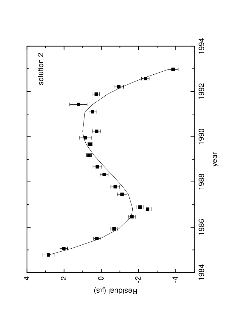
Figure 2: The scattered points are measured by Kaspi et al. (1994), the solid line is given by the orbital precession model.

Figure 3: The scattered points are measured by Kaspi et al. (1994), the solid line is given by the orbital precession model.

References

- (1) Alpar,M.A., Cheng,A.F.,Ruderman, M.A., Shaham,J. 1982, Nature, 300, 728
- (2) Apostolatos,T.A., Cutler,C., Sussman,J.J., Thorne,K.S., 1994, Phys. Rev. D, 49,6274
- (3) Arzoumanian,Z., Fruchter,A.S., Taylor,J.H. 1994, ApJ, 426, L85
- (4) Backer, D.C., Kulkarni,S.R., Heiles,C., Davis, M.M. Goss, W.M. 1982, Nature 300, 615
- (5) Barker, B.M., O’Connel, R.F., 1975, Phys. Rev. D, 12, 329
- (6) Bhattacharya, D., van den Heuvel, E.P.J. 1991,Phys. Rep.,203.1
- (7) Doroshenko,O., Löhmer,O.,Kramer, M., Jessner,A., Wielebinski,R. Lyne,A.G., Lange, Ch., 2001, A&A, 379, 579
- (8) Hamilton, A.J.S., Sarazin,C.L., 1982 MNRAS, 198, 59
- (9) Gong, B.P.(1) 2003, Astro-ph/0308286
- (10) Gong, B.P.(2) 2003, Astro-ph/0303027
- (11) Gong, B.P.(3) 2003, Astro-ph/0306078
- (12) Kaspi, V.M., Taylor, J.H., Ryba, M.F. 1994, ApJ, 428, 713
- (13) Kidder,L.E., 1995, Phys. Rev. D, 52, 821
- (14) King, A.R., Davies, M.B., Beer, M.E. 2003, MNRAS, to be appeared.
- (15) Konacki,M., Wolszczan,A., Stairs, I.H. 2003, ApJ, 589, 495
- (16) Manchester, R.N., Taylor, J.H. 1977, Pulsars, Freeman and Company San Francisco.
- (17) Shapiro,S.L., Teukolsky,S.A. 1983, Black Holes, White Dwarfs, and Neutron Stars, John Wiley Sons.
- (18) Smarr,L.L., Blandford, R.D., 1976, ApJ, 207, 574
- (19) Taylor, J. H. Weisberg, J. M. 1989, ApJ. 345, 434.
- (20) Thorsett, S,E. Phillips,J.A. 1992, ApJ, 387, L69
- (21) Wex,N., Kopeikin, S.M. 1999, ApJ., 514, 388