Simultaneous determination of $\Omega_{\rm M0}$ and $H_{0}$ from joint Sunyaev-Zeldovich effect and X-ray observations with median statistics

Clusters of galaxies contain a fair sample of the universal baryonic mass fraction. A combined analysis of the intracluster medium (ICM) within their hydrostatic regions, as derived from both Sunyaev-Zeldovich effect (SZE) measurements and X-ray images, makes it possible to constrain the cosmological parameters. We consider both gas fraction estimates and angular diameter distance measurements. Adopting median statistics, we find, at the 2-$\sigma$ level, the pressureless matter density, $\Omega_{\rm M0}$, to be between 0.30 and 0.40 and the Hubble constant, $H_{0}$, between 44 and 66 Km s^-1 Mpc^-1.

1 Introduction

Rich clusters of galaxies are the largest known virialized structures in the Universe. Their importance in observational cosmology is known from early times. In the beginning of the last century, direct estimates of their total masses first stated the need for unseen dark matter (Zwicky zwi33 (1933)). Now, they continue to provide important information to characterize the Universe (see, for example, Wang et al. wan+al00 (2000); Sereno io02cl (2002)).

A method, independent of the nature of the dark matter and based on minimal assumptions, to constrain the geometry of the Universe and its matter and energy content is based on gas mass observations in clusters of galaxies.

As shown with X-ray and optical imaging, the main contribution to the baryonic budget in clusters of galaxies is provided by the hot gaseous intracluster medium (ICM). The gas mass is about an order of magnitude larger than the mass in stars in cluster galaxies and provides a reasonable estimate of the cluster’s baryonic mass (Fukugita et al. fuk+al98 (1998); Lin et al. lin+al03 (2003)).

The ICM is X-ray emitting via thermal bremsstrahlung and produces a spectral distortion of the cosmic microwave background radiation (CMBR), known as Sunyaev-Zeldovich effect (SZE) (Sunyaev & Zeldovich sun+zel70 (1970); Birkinshaw birk99 (1999)). The SZE is proportional to the pressure integrated along the line of sight, i.e. to the first power of the gas density. X-ray emission depends on the second power of the density. The ICM mass fraction may be estimated from either of these, fundamentally different, observables, based on independent techniques.

Since there is no efficient way to change the baryon fraction averaged within a Mpc scale, the mass composition in clusters, when estimated out to a standard hydrostatic radius, is expected to reflect the universal mass composition (White et al. whi+al93 (1993); Sasaki sas96 (1996); Evrard evr97 (1997)). Precise measurements of the visible baryonic mass fraction in galaxy clusters, $f_{\rm B}$, along with our knowledge of the universal baryonic density parameter, $\Omega_{\rm B0}$, provides a physically based technique for estimating cosmological parameters (White et al. whi+al93 (1993)). Ratio of the ICM mass to the total mass of the cluster represents a first estimate of $f_{\rm B}$. So, a useful constraint on the cosmological parameters is given by the identity $\Omega_{\rm M0}=\Omega_{\rm B0}/f_{\rm B}$. Independent estimates of $f_{\rm B}$ can be obtained either from SZE measurements or X-ray imaging observations. The angular diameter distance, where the dependence on the cosmological parameters appears, to the cluster enters in the two gas mass estimates through a characteristic length-scale of the cluster along the line of sight. From the different dependencies of SZE and X-ray emission on the density of ICM, different dependencies on the assumed cosmology are implied.

Galaxy cluster gas mass fractions from SZE measurements have been used in Grego et al. (gre+al01 (2001)) to constrain $\Omega_{\rm M0}$. X-ray gas mass fraction in relaxed clusters have provided upper limit on the cosmological density parameter (Mohr et al. moh+al99 (1999); Ettori & Fabian ett+fab99 (1999); Allen et al. all+al02 (2002); Erdogdu et al. erd+al02 (2002); Ettori et al. ett+al02 (2002)).

Without referring to the universal baryonic fraction, with some assumptions about the geometry of the cluster, a joint analysis of SZE measurements with X-ray imaging observations, since the different density dependencies, makes it possible to determine the distance to the cluster. Such a distance, independent of the extragalactic distance ladder, is then used to measure the Hubble constant (Birkinshaw birk99 (1999); Mason et al. mas+al01 (2001); Jones et al. jon+al02 (2002); Reese et al. ree+al02 (2002)).

All of the methods discussed above are based on ICM mass observations. Estimates of gas mass depend on the cosmological parameters through the angular diameter distance to the cluster. Equating the gas fraction in cluster to the universal baryonic fraction allows to investigate both the Hubble constant and the cosmological density parameters. Taking advantage of the different density dependencies, SZE and X-ray observations provide independent constraints in the space of cosmological parameters, leading one to solve for two unknowns at the same time.

Distance measurements are obtained by equating the central densities as derived from SZE and X-ray methods. Instead of equating the gas fraction to an universal value, now the two gas mass estimates are forced to coincide each other. This constraint is independent and nearly orthogonal to the previous ones and allows to solve for an additional unknown.

Usually, when deriving cosmological constraints from gas mass fractions, in order to estimate $\Omega_{\rm M0}$, a prior on the Hubble constant is assumed. On the other hand, using the cosmic distance scale from interferometric measurements of the SZE to determine $H_{0}$ requires, with the current data sets, to fix the background cosmology. We show how a joint analysis of all the information on the ICM from both SZE and X-ray measurements enables to determine, at the same time, $\Omega_{\rm M0}$ and $H_{0}$.

The quality of the data samples used in the analysis determines the area of the overlapping region and the precision of the estimate. We perform a combined analysis of data samples, available in literature, of SZE measurements and X-ray observations.

Since we have to combine different data sets, obtained with independent methods, we adopt median statistics. As shown in Gott et al. (got+al01 (2001), see also Avelino et al. ave+al02 (2002) and Chen & Ratra ch+ra03 (2003)), median statistics provide a powerful alternative to $\chi^{2}$ likelihood methods with fewer assumptions about the data. Statistical errors are not required to be known and Gaussianly distributed. Since errors, as reported in X-ray and SZE literature, are usually asymmetric, performing an analysis without using the errors themselves turns out to be a very conservative approach. Furthermore, median statistics is also less vulnerable to the presence of bad data and outliers. Since we are proposing a method to constrain cosmology with ICM mass estimates which extend and combine methods previously established, in this early stage we think that median statistics can be the best choice.

In Section 2, we derive the dependence of the ICM gas mass, derived from X-ray observations or SZE measurements, on the assumed cosmological parameters. In Section 3, the data samples and our selection criteria on the clusters are presented. In Section 4, the median statistics is shortly presented and the results are listed. Section 5 is devoted to the discussion of various systematic uncertainties. Conclusions are in Section 6.

2 The gas mass estimate

The ICM mass is calculated by integrating the ICM density profile, $\rho_{\rm ICM}$, over an assumed shape,

$$M_{\rm ICM}(V)=\int_{V}\rho_{\rm ICM}(\@vec{r})d^{3}\@vec{r}\propto m_{\rm p}\int_{V}n_{\rm e}(\@vec{r})d^{3}\@vec{r},$$ (1)

where $n_{\rm e}$ is the electron number density profile and $m_{p}$ is the proton mass. For a spherically symmetric system, like the widely used $\beta$-model (Cavaliere & Fusco cav+fus76 (1976, 1978)), the mass within a fixed metric radius $r$ is

$$M_{\rm ICM}\propto n_{\rm e0}r^{3},$$ (2)

where $n_{\rm e0}$ is the central number density. The radius $r$ can be expressed as the product of an observable angular radius by the angular diameter distance to the cluster, $d_{\rm A}$.

The central number density can be measured by fitting the X-ray surface brightness profile, $S_{\rm X}\propto\int n_{\rm e}^{2}\Lambda(T_{\rm e})dl$, where the integration is along the line of sight and $\Lambda(T_{\rm e})$ is the X-ray emissivity at the electronic temperature $T_{\rm e}$. The dependence on distance is made explicit by expressing the integration variable in a dimensionless form, $dl=d_{\rm A}d\zeta$. It comes out

$$n_{\rm e0}^{X}\propto\sqrt{\frac{S_{\rm X}}{d_{\rm A}}},$$ (3)

so, for the gas mass, when measured with X-ray observations, it is

$$M_{\rm ICM}^{X}\propto d_{\rm A}^{5/2}.$$ (4)

Spatially resolved measurements of the SZE can also determine $n_{\rm e0}$. Since the brightness temperature decrement of the CMBR towards a cluster is expressed as $\frac{\Delta T_{\rm SZ}}{T_{\rm CMBR}}\propto\int n_{\rm e}T_{\rm e}dl$, then

$$n_{\rm e0}^{\rm SZ}\propto\frac{\Delta T_{\rm SZ}}{T_{\rm CMBR}}\frac{1}{d_{\rm A}};$$ (5)

so, it is

$$M_{\rm ICM}^{\rm SZ}\propto d_{\rm A}^{2}.$$ (6)

The temperatures generally taken in analyses are the X-ray emission weighted temperatures, usually measured over a few core radii. If the temperature has a spatial structure, the temperature inferred from such an average procedure may depend on how much of the cluster is considered. This can lead to a substantial change in the SZE inferred, and thus to a systematic error in the determination of the cosmological parameters (Majumdar & Nath ma+na00 (2000)).

Typically, an estimate of the total mass of a cluster of galaxies is obtained under the assumption that the gas, supported solely by thermal pressure, is in hydrostatic equilibrium in the cluster’s gravitational potential. Assuming spherical symmetry and isothermal gas, the total mass of a cluster within radius $r$ is

$$M_{\rm TOT}(<r)=\frac{k_{\rm B}T_{\rm X}r}{G\mu m_{\rm p}}\frac{d\log n_{\rm e}(r)}{d\log r}\propto d_{\rm A},$$ (7)

where $k_{\rm B}$ is the Boltzmann’s constant, $\mu m_{\rm p}$ is the mean molecular weight of the gas and $T_{\rm X}$ is the spatially averaged X-ray emission temperature of the gas determined from a broad-beam spectroscopic instrument. Combining Eqs. (4, 6) with Eq. (7), the two estimates of the ICM mass fraction turn out

$$f_{\rm ICM}\equiv\frac{M_{\rm ICM}}{M_{\rm TOT}}\propto d_{\rm A}^{\beta},$$ (8)

where, for X-ray observations, $\beta_{\rm X}=3/2$ and, for SZE data, $\beta_{\rm SZ}=1$.

By eliminating $n_{\rm e0}$ from Eqs. (3, 5), one can solve for the angular diameter distance, yielding

$$d_{\rm A}\propto\frac{\Delta T_{\rm SZ}^{2}}{S_{\rm X}}.$$ (9)

The derived values of $f_{\rm ICM}$ depend on the cosmological parameters through the angular diameter distances (Sasaki sas96 (1996)). In a Friedmann-Lemaître-Robertson-Walker universe filled in with pressureless matter and a cosmological constant, the angular diameter distance to a source at redshift $z$ is

$$d_{\rm A}(z)=\frac{c}{H_{0}}\frac{1}{|\Omega_{\rm K0}|^{1/2}(1+z)}$$

$${\times}{\rm Sinn}\left\{\int_{0}^{z}\frac{|\Omega_{\rm K0}|^{1/2}}{\sqrt{\Omega_{\rm M0}(1+z^{{}^{\prime}})^{3}+\Omega_{\Lambda 0}+\Omega_{\rm K0}(1+z^{{}^{\prime}})^{2}}}dz^{{}^{\prime}}\right\},$$

where $\Omega_{\Lambda 0}$ is the reduced cosmological constant, $\Omega_{\rm K0}=1-\Omega_{\rm M0}-\Omega_{\Lambda 0}$, and ${\rm Sinn}(x)$ is $\sinh(x)$, $x$, $\sin(x)$ for $\Omega_{\rm K0}$ greater than, equal to and less than zero, respectively; $H_{0}$ is the today Hubble constant. For the expression of the distance in inhomogeneous universes we refer to Sereno et al. (ser+al01 (2001), ser+al02 (2002)). In the next, we will consider only the flat case, $\Omega_{\rm K0}=0$, strongly supported by the bulk of evidences (de Bernardis et al. deb+al00 (2000); Harun-or-Rashid & Roos ha+ro01 (2001)).

To compare the ICM mass fraction of different clusters, we have to study the same portion of the virial region in each cluster. In such a region, we expect all clusters to have the same gas fraction and the gas to be isothermal. Regions of different clusters are characterized by the same properties if they encompass the same mean interior density contrast, $\delta_{\rm c}$, with respect to the critical density at their own redshit, $\rho_{\rm c}(z)\equiv\frac{3H^{2}(z)}{8\pi G}$, as strongly suggested by numerical simulation (Evrard et al. evr+al96 (1996); Frenk et al. fre+al99 (1999)); $H(z)$ is the redshift dependent Hubble constant,

$$H(z)=H_{0}\sqrt{\Omega_{\rm M0}(1+z)^{3}+\Omega_{\Lambda 0}+\Omega_{\rm K0}(1+z)^{2}}\ .$$ (11)

The density contrast $\delta_{\rm c}$ is attained at the radius $r_{\delta_{\rm c}}$ (Evrard et al. evr+al96 (1996); Evrard evr97 (1997)). According to an analysis of gas velocity moments (Evrard et al. evr+al96 (1996)), $\delta_{\rm c}=500$ is a conservative estimate of the boundary between the inner, nearly hydrostatic and virialized central region of the cluster and the surrounding, recently accreting outer envelope. Clusters of different temperatures have similar structures once scaled to $r_{500}$, within which the easily visible region of the cluster is also probed with the typical background sensitivity. Hydrodynamical simulations (Evrard et al. evr+al96 (1996)) also show that the assumption of an isothermal gas in hydrostatic equilibrium is valid within the virial radius.

The virial equilibrium expectations at a fixed density contrast, that is

$$T\sim\frac{GM}{r_{\delta_{\rm c}}}\propto\frac{\delta_{\rm c}\rho_{\rm c}r_{\delta_{\rm c}}^{3}}{r_{\delta_{\rm c}}}\propto\delta_{\rm c}H^{2}(z)r_{\delta_{\rm c}}^{2},$$ (12)

can be calibrated by means of numerical simulation (Evrard et al. evr+al96 (1996)),

$$r_{500}(T_{\rm X})=r_{10}(500,\Omega_{\rm M0})\left(\frac{T_{\rm X}}{\rm{10KeV}}\frac{H_{0}^{2}}{H^{2}(z)}\right)^{1/2}\frac{1}{h},$$ (13)

where $h$ is $H_{0}$ in units of 100 km s^-1Mpc^-1. The normalization $r_{10}$ in Eq. (13) is the average radial scale of $10$ KeV clusters at density contrast $\delta_{\rm c}=500$. Since the scaling law reflects the virial equilibrium within $\delta_{\rm c}\sim{\cal{O}}(10^{3})$, $r_{10}(500)$ is nearly insensitive to the peculiar cosmology. We put $r_{10}(500,\Omega_{\rm M0})=1.24\pm 0.08$ Mpc (Evrard et al. evr+al96 (1996)).

The gas fraction at $r_{500}$, once known at a fixed physical radius $r_{\rm X}$, can be evaluated using a mild, power law extrapolation of the data quoted at $r_{\rm X}$ (Evrard evr97 (1997)),

$$f_{\rm ICM}[r_{500}(T_{\rm X})]=f_{\rm ICM}(r_{\rm X})\left[\frac{r_{500}(T_{\rm X})}{r_{\rm X}}\right]^{\eta},$$ (14)

with $\eta=0.17$ as derived from numerical simulations (Evrard et al. evr+al96 (1996)). The small value of $\eta$ also reduces the error on the gas fraction which propagates from an uncertain determination of the normalization factor in Eq. (13). Using a different normalization based on observations of the relatively relaxed cluster A1795, Mohr et al. (moh+al99 (1999)) found $r_{10}(500)\approx 1.19$. Since $\eta=0.17$, the relative variation on $f_{\rm ICM}(500)$ between the two normalization is less then $1\%$.

Present X-ray observations are mostly sensitive to the inner cluster regions, but, future SZE data would probe more exterior region, allowing an analysis on larger scales. There are some evidences that the gas fraction increases by about 15% from $r_{500}$ to $r_{200}$ (Ettori & Fabian ett+fab99 (1999)). Since the currently derived gas fraction profile increases regularly from the inner part to the outer part, up to the virial radius and beyond (Sadat & Blanchard sad+bla01 (2001)), the $\eta$ value at $\delta_{\rm c}\ll 500$ accordingly changes but, whenever the ratio of $r_{\delta_{\rm c}}$ and $r_{\rm X}$ is within few percent of each other, the effect of $\eta$ on the final result is really negligible (Cooray 1998a ).

The variations in the gas fraction within the virial regions are then quite small. At a given temperature, the scatter in $f_{\rm ICM}$ is less than $20\%$, including both intrinsic variations and measurements errors (Arnaud & Evrard arn+evr99 (1999); Vikhlinin vik+al99 (1998)).

The estimated gas mass fraction out to $r_{500}$ depends on cosmology through the angular diameter distance, see Eq. (8), and the time dependent Hubble constant, see Eq. (13). From Eqs. (8, 13, 14), we get

$$f_{\rm ICM}[r_{500}]\propto d_{\rm A}^{\beta-\eta}H(z)^{-\eta}.$$ (15)

$f_{\rm ICM}[r_{500}]$ is a decreasing function of both $\Omega_{\rm M0}$ and $H_{0}$. So, an increment in $\eta$ determines an overestimate of these cosmological parameters.

Under the assumption that the gas fraction is time independent and constant for all clusters, it is possible to constrain the cosmological parameters (Sasaki sas96 (1996); Pen pen97 (1997); Cooray 1998a ; Danos & Pen dan+pen98 (1998); Rines et al. rin+al99 (1999)). The evolution of the gas mass fraction is still under discussion (Schindler schi99 (1999); Ettori & Fabian ett+fab99 (1999); Roussel et al. rou+al00 (2000)). An observed variation of $f_{\rm ICM}$ with the redshift would be explained by a wrong assumption for the angular diameter distance and the cosmological parameters and/or a true time evolution. In the near future, the study of the power spectrum of the secondary CMBR anisotropies due to the thermal SZE by clusters of galaxies should give a discriminatory signature of any possible evolution of the ICM mass fraction (Majumdar maju01 (2001)); however, at the moment, numerical simulations do not suggest any evolution.

3 Data sample

The observational sample we consider is based on the X-ray data set in Mohr et al. (moh+al99 (1999), hereafter MME) and Ettori & Fabian  (ett+fab99 (1999); EF), on the SZE data from Grego et al. (gre+al01 (2001); GCR), and on the joint analysis of interferometric SZE observations with X-ray imaging observations in Reese et al. (ree+al02 (2002); RCJ). All the published ICM mass fractions are given out to an angular radius within which the signal-to-noise ratio is good enough and the problems deriving from extrapolation procedure are really negligible (Sadat & Blanchard sad+bla01 (2001)).

In order to work with a homogeneous sample, we impose a cut on the temperature, requiring $T_{\rm X}>5$ KeV. Cluster evolution is not an entirely self similar process driven exclusively by gravitational instability (David et al. dav+al95 (1995); Ponman et al. pon+al96 (1996); MME). While massive clusters are less affected by processes like galaxy feedback, low mass clusters may have lost gas as a result of preheating and post-collapse energy input, so enhancing ICM depletion within the virial region. The net result is that the ICM mass fraction shows a mild increasing trend with the temperature. Both observations (MME) and numerical simulations of the effect of preheating (Bialek et al. bia+al01 (2001)) show that $f_{\rm B}$ is depressed below the cosmic mean baryon fraction in clusters with $T_{\rm X}\stackrel{{\scriptstyle<}}{{\sim}}3$ KeV. However, the trend between $f_{\rm B}$ and $T_{\rm X}$ is not clear (Roussel et al. rou+al00 (2000)) and an analysis in Arnaud & Evrard (arn+evr99 (1999)) of selected clusters with weak cooling flow does not give clear statistical significance. Sanderson et al (san+al03 (2003)) found departures from a self-similar behaviour in the scaling properties of a large sample of virialized haloes. Both the relation between the gas density slope parameter and the temperature and the gas fraction data reveal a flattening of the gas density profiles in small sized haloes, consistent with energy injection into the ICM by non-gravitational means. A clear trend for cooler system to have a smaller gas fraction emerged, although, above 4 KeV, the significance of this correlation is weakened.

To be more conservative with respect to these shortcomings, we consider only clusters with $T_{\rm X}>5$ KeV, which are less affected by feedback from galaxy formation and where $f_{\rm ICM}$ appears to be constant without opposite claims. This criterion is passed by $28$ clusters from the sample in MME, $35$ from the sample in EF, $18$ from both the sample in GRC and RCJ

4 Data analysis

Median statistics provide a powerful tool to experimental data analysis. Few assumptions about the data and their errors are required. Usual $\chi^{2}$ statistics assume that i) experimental data are statistically independent; ii) there are no systematic effects; iii) experimental errors are Gaussianly distributed; iv) the standard deviation of these errors is known. On the other hand, median statistics assume only hypotheses i) and ii).

To compute the likelihood of a particular set of cosmological parameters, we count how many data points are above or below each cosmological model prediction and compute the binomial likelihoods. Given a binomial distribution, if we perform $N$ measurements, the probability of obtaining $k$ of them above the median is given by

$$P(k)=\frac{2^{-N}N!}{k!(N-k)!}.$$ (16)

We perform such a test on the baryonic gas fraction measured with X-ray data from MME and EF, on the gas mass fraction from SZE observations from GCR and, finally, on the cosmological distances measurements in RCJ

4.1 Baryonic mass fractions

We count the number of baryon mass fractions that are too heavy with respect to (i.e. greater than) the ratio $\Omega_{\rm B0}/\Omega_{\rm M0}$. ICM is not the only contribution to the cluster baryon budget. Other contributions come from the luminous mass in galaxies, intergalactic stars and a hypothetical baryonic dark matter. While the latter two terms can be neglected (Ettori et al. etto01 (2001)), the typical stellar contribution to the baryonic mass is between $5$ and $20\%$ (White et al. whi+al93 (1993); Fukugita et al. fuk+al98 (1998); Roussel et al. rou+al00 (2000)). The ICM is the most extended mass component in clusters, while the galaxies are the most centrally concentrated one (David et al. dav+al95 (1995)). There are some indications of a trend of increasing gas mass fraction and decreasing mass in optically luminous matter with increasing mass of the clusters (David et al. dav+al95 (1995); David dav+al95 (1995)), but this claim is still debated (Roussel et al. rou+al00 (2000)). Lin et al. (lin+al03 (2003)) found that the total baryon fraction is an increasing function of the cluster mass. Estimating the stellar mass using $K$-band luminosity, they also showed how the ICM to stellar mass ratio nearly doubles from low- to high-mass clusters. However, our choice to consider only massive clusters with $T_{\rm X}>5$ KeV gives some cautions in considering the total mass in galaxies as a fixed fraction of the cluster gas. We have adopted the estimate in Fukugita et al. (fuk+al98 (1998)), $f_{\rm B}=(1+\left[0.18^{+0.10}_{-0.08}\right]h^{1/2})f_{\rm ICM}$.

A determination for $\Omega_{\rm B0}$ is required. One of the most precise determination of the physical baryonic density is derived in O’Meara et al. (ome+al01 (2001)). By combining measurements of the primeval abundance of deuterium, as inferred from high-redshift Ly$\alpha$ systems, and theoretical predictions of the big-bang nucleosynthesis, they found $\Omega_{\rm B0}h^{2}=0.0205{\pm}0.0018$. Measurements of the angular power spectrum of the CMBR also provide an estimate of the baryon abundance. For the recent WMAP data (Spergel et al. spe+al03 (2003)), $\Omega_{\rm B0}h^{2}=0.024{\pm}0.001$, depending primarily on the ratio of the first to second peak heights. When combined with other finer CMBR experiments and 2dFGRS measurements, WMAP data gives $\Omega_{\rm B0}h^{2}=0.022{\pm}0.001$ (Spergel et al. spe+al03 (2003)), in remarkable agreement with the result from Ly$\alpha$ forest data. CMBR predictions depend on a multi-dimensional fitting procedure involving all the cosmological parameters together, included the parameters we want to determine, i.e. $H_{0}$ and $\Omega_{\rm M0}$, so we prefer to adopt the estimate from O’Meara et al. (ome+al01 (2001)).

The ICM mass fraction in Eq. (15) is a decreasing function of both $H_{0}$ and $\Omega_{\rm M0}$, so, increasing the observed value of the baryon abundance, i.e. $\Omega_{\rm B0}$, determines an underestimate of both $H_{0}$ and $\Omega_{\rm M0}$.

We use the ICM mass fractions to a fixed metric radius as reported in Table 4 in MME, Table  2 in EF and Table 4 in GCR. Then, we extrapolate to the virial radius assuming the reference cosmological model ($\Omega_{\rm M0}=1$ and $h=0.5$ in MME and in EF and $\Omega_{\rm M0}=0.3$ and $h=1$ in GCR); the prediction of a generic cosmological model is obtained according to Eq. (15). We join the X-ray derived mass fraction lists in MME and EF in a single data sample with 63 data points. The 1-$\sigma$ and region 2-$\sigma$ in the $\Omega_{\rm M0}$-$h$ plane are located by cosmological pairs whose predictions are between 28 and 35 times ($68.65\%$ confidence region) or between 24 and 39 times ($95.70\%$), respectively, above $\Omega_{\rm B0}/\Omega_{\rm M0}$.

The SZE derived mass fraction data sample provides 18 entries. Now, the 1-$\sigma$ and 2-$\sigma$ regions in the $\Omega_{\rm M0}$-$h$ plane are located by points with a number of overestimates between 7 and 11 ($76.2\%$) and 5 and 13 ($96.9\%$), respectively. Since the different dependence on the cosmological parameters, the results from X-ray and SZE measurements locate independent regions in the $\Omega_{\rm M0}$-$h$ plane, see Fig. (1). In any case the points in the SZE sample are not enough to significantly constrain cosmological parameters from estimates of gas fraction alone.

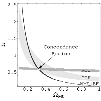
Figure 1: Concordance region (white) at the 1-$\sigma$ level. Different gray-scaled patches show constraints from different data samples. Regions labelled with RCJ, GRC and MME+EF denote constraints from cosmological distances, baryonic mass fractions from SZE measurements and baryonic mass fractions from X-ray data, respectively.

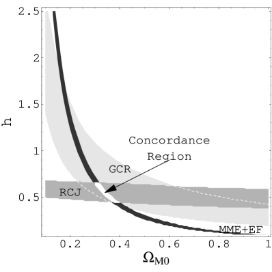
Figure 2: Concordance region (white) at the 2-$\sigma$ level. Different gray-scaled patches show constraints from different data samples. Regions labelled with RCJ, GRC and MME+EF denote constraints from cosmological distances, baryonic mass fractions from SZE measurements and baryonic mass fractions from X-ray data, respectively.

4.2 Cosmological distances

As seen in Section 2, when combining X-ray and SZE data, a third constrain can be obtained without referring to any value of $\Omega_{\rm B0}$. Reese et al. (ree+al02 (2002)) determined the distances to 18 galaxy clusters with redshift ranging from $z\sim 0.14$ to $0.78$. Now, for each cosmological model, we count the number of clusters that are too distant, i.e the number of cluster whose distance calculated according to Eq. (2) for a set of cosmological parameters is greater than the measured value. The confidence region in the $\Omega_{\rm M0}$-$h$ plane are determined with the same criteria as for the SZE derived mass fraction. Despite the numbers of entries for the cosmological distances and for the baryonic mass fraction from SZE data are the same, the former does better since the difference dependence on cosmological parameters. The test on the cosmological distances, very sensitive to the Hubble constant, provides a nearly orthogonal constraint to the method of the baryonic fraction. At the 1-$\sigma$ level, we get $0.50\stackrel{{\scriptstyle<}}{{\sim}}h\stackrel{{\scriptstyle<}}{{\sim}}0.66$; the 2-$\sigma$ confidence range is $0.38\stackrel{{\scriptstyle<}}{{\sim}}h\stackrel{{\scriptstyle<}}{{\sim}}0.70$. Using a $\chi^{2}$ statistics, where the statistical uncertainties have been obtained combining in quadrature and then averaging not Gaussian, asymmetric errors, Reese et al. (ree+al02 (2002)) found, as $68.3\%$ confidence range, $0.51\stackrel{{\scriptstyle<}}{{\sim}}h\stackrel{{\scriptstyle<}}{{\sim}}0.64$, nearly as constraining as our result.

4.3 Concordance analysis

To evaluate the allowed range of $\Omega_{\rm M0}$ and $h$, we have to consider together the three independent constraints. We apply a concordance analysis, only retaining the pairs of cosmological parameters which lie within 1-$\sigma$ or 2-$\sigma$ of each individual constraint (Wang et al. wan+al00 (2000)). This procedure is conservative with respect to possibly not well controlled systematic errors and puts in evidence the most effective constraints in delimiting the allowed range. As can be seen from Figs. (1, 2), constraints from cosmological baryonic fraction are nearly orthogonal to that from cosmological distances. At the 1-$\sigma$ level, Fig. (1), we get $0.31\stackrel{{\scriptstyle<}}{{\sim}}\Omega_{\rm M0}\stackrel{{\scriptstyle<}}{{\sim}}0.34$ and $0.55\stackrel{{\scriptstyle<}}{{\sim}}h\stackrel{{\scriptstyle<}}{{\sim}}0.62$. At the 2-$\sigma$ level, Fig. (2), we get $0.30\stackrel{{\scriptstyle<}}{{\sim}}\Omega_{\rm M0}\stackrel{{\scriptstyle<}}{{\sim}}0.40$ and $0.44\stackrel{{\scriptstyle<}}{{\sim}}h\stackrel{{\scriptstyle<}}{{\sim}}0.66$.

5 Systematic effects

Several systematic uncertainties are involved when deriving cosmological parameters from the cluster gas mass observations.

5.1 ICM depletion

Shocks during cluster formation can drive an ICM depletion within $r_{500}$. Numerical simulations (Frenk et al.  fre+al99 (1999)) and observations (Sanderson et al. san+al03 (2003)) show that the gas distribution is more extended than the dark matter one. The extended gas structure implies a weakly rising baryon fraction with radius (Evrard evr97 (1997); EF), $f_{\rm ICM}\sim r^{\eta}$, see Eq. (14), and this increasing trend is stronger in less massive clusters (Schindler schi99 (1999)). The ratio $\Upsilon$ of the enclosed baryon fraction to the universal cosmic value within a fixed density contrast,

$$\Upsilon(\delta_{\rm c})\equiv\left(\frac{\Omega_{\rm B0}}{\Omega_{\rm M0}}\frac{1}{f_{\rm B}(\delta_{\rm c})}\right)^{-1},$$ (17)

has been calibrated by simulations. A modest overall baryonic diminution, about $10\%$, has been found (Evrard evr97 (1997); Frenk et al. fre+al99 (1999)).

5.2 Density clumping

Small-scale density fluctuations on X-ray measurements of the ICM mass arising from accretion events and major mergers can introduce a bias in the determination of $f_{\rm ICM}^{X}$. Density clumping on a scale less than the resolution of the images causes an enhancement of the X-ray brightness by a factor $C_{\rm n}=\langle n_{\rm e}^{2}\rangle/\langle n_{\rm e}\rangle^{2}$ with respect to a uniform smooth atmosphere. Since the surface brightness profile is proportional to the square of the central gas density, see Eq. (3), $f_{\rm ICM}^{X}$ is overestimated by $C_{\rm n}^{1/2}$. Numerical hydro-simulations show that $C_{\rm n}^{1/2}=1.16\pm 0.01$ (Mathiesen et al. mat+al99 (1999)). However, the spread in this value, on a cluster-by-cluster basis, can be much larger than this.

Since the value of $\langle n_{\rm e}\rangle$ is not changed by density clumping, the estimate of $f_{\rm ICM}$ based on the SZE is not affected by this systematic effect.

Currently, there is no observational evidence of significant clumping in galaxy clusters (RCJ).

5.3 Other effects

Several other systematic effects can affect the gas mass fraction measurements. A magnetic field in the cluster plasma might support a non thermal component in the X-ray emission. It can be effective in the core regions of the cluster but it is unlikely that it plays a major role out to the hydrostatic radius (Cooray 1998a ). The non-isothermality of the ICM has also been taken into account (Ettori et al. etto01 (2001); Puy et al. puy+al00 (2000)). The presence of a temperature gradient increases the gas fraction estimated at the virial radius $r_{500}$, whereas correcting by the contamination of a magnetic field reduces $f_{\rm ICM}$ (Ettori et al. etto01 (2001)).

Heating and cooling process may also act in galaxy clusters, but they do not change in a significant way the estimate of the mean $f_{\rm ICM}$ in a numerous enough cluster sample (Cooray 1998a ). Cooling processes can alter the ICM profiles. Since the SZE depends essentially on the pressure profile, a cooling flow can lead to an underestimation of the cosmological distance (Majumdar & Nath ma+na00 (2000)). Even after excluding $\sim 80\%$ of the cooling-flow region from the analysis, a $\sim 10\%$ overestimation of $H_{0}$ may be in order.

Cluster geometry introduces an important uncertainty in SZE- and X-ray-derived quantities (Cooray 1998b ; Puy et al. puy+al00 (2000)). Complicated cluster structure and projection effects cannot currently be disentangled. Projection effects of aspherical cluster modelled with a spherical geometry broaden the distribution of measured gas mass fraction and should be corrected by taking into account the distribution of ellipticities for the cluster sample (Cooray 1998b ). The effects of asphericity contribute significantly to the distance uncertainty for each cluster, but the determination of the Hubble constant from a large sample of clusters is not believed to be significantly biased (RCJ).

These various effects do not act all in the same direction; furthermore, they require a very detailed modelling in order to correct for a not very significant amount. Since an ensemble of hydro-dynamical cluster simulations has shown that the departures from an isothermal, spherical ICM do not introduce serious errors (GRC), we have not considered them in our analysis.

Considering the effects discussed in Section (5.1, 5.2), ICM mass fraction should be corrected according to

$$f_{\rm B}^{\rm X}=f_{\rm ICM}^{X}\left[1+\frac{f_{\rm gal}}{f_{\rm ICM}}\right]\frac{1}{\Upsilon(500)}\frac{1}{C_{\rm n}^{1/2}},$$ (18)

and

$$f_{\rm B}^{\rm SZ}=f_{\rm ICM}^{\rm SZ}\left[1+\frac{f_{\rm gal}}{f_{\rm ICM}}\right]\frac{1}{\Upsilon(500)}.$$ (19)

6 Conclusions

The simple argument presented here, based on the different dependence of the galaxy cluster ICM mass estimates on the cosmological parameters as derived either from SZE measurements or from X-ray observations, has made it possible to infer both the value of the pressureless matter density parameter and the Hubble constant. The only additional information is the value of the universal baryonic matter density. To our knowledge, this is the first time that gas mass estimates are used to derive $\Omega_{\rm M0}$ and $H_{0}$ together.

We have followed median statistics. This technique assumes only that the measurements are independent and free of systematic errors. Physical quantities in literature, such as X-ray emission temperature ICM mass fractions and cosmological distances, are often presented with asymmetric errors bars. Supposing these errors following a Gaussian distribution with known standard deviation, as required by usual $\chi^{2}$ analysis, is a hard hypothesis. On the other hand, median statistics, based on fewer assumptions, can provide very interesting and constraining results, as shown in several astrophysical cases (Gott et al. got+al01 (2001); Avelino et al. ave+al02 (2002); Chen & Ratra ch+ra03 (2003)). To minimize the role of systematic uncertainties, we have performed a concordance analysis of the data (Wang et al. wan+al00 (2000)).

Our estimates agree with the currently favoured model of Universe (Wang et al. wan+al00 (2000)), derived from observational constraints such as measurements of the anisotropy of the CMBR (Spergel et al. spe+al03 (2003)), large-scale structure observations (Peacock et al. pe&al01 (2001))and evidences coming from type Ia supernovae (Riess et al. ri&al98 (1998); Perlmutter et al. pe&al99 (1999)).

We have found a value of $\Omega_{\rm M0}$ in full agreement with the bulk of evidences (Harun-or-Rashid & Roos ha+ro01 (2001); Chen & Ratra ch+ra03 (2003)). Median statistics analyses of various collections of measurements has been used in Chen & Ratra (ch+ra03 (2003)) to determine an estimate of $\Omega_{\rm M0}$. They found $0.20\stackrel{{\scriptstyle<}}{{\sim}}\Omega_{\rm M0}\stackrel{{\scriptstyle<}}{{\sim}}0.35$ at two standard deviations, in full agreement with our estimate $0.30\stackrel{{\scriptstyle<}}{{\sim}}\Omega_{\rm M0}\stackrel{{\scriptstyle<}}{{\sim}}0.40$.

Our determination of the Hubble constant is independent of the local extragalactic distance scale. We find $0.44\stackrel{{\scriptstyle<}}{{\sim}}h\stackrel{{\scriptstyle<}}{{\sim}}0.66$ at 2-$\sigma$, in agreement with the estimate of the Hubble Space Telescope Key Project, $h=0.72{\pm}8$ (Freedman et al. fre+al01 (2001)). Together with SZE-derived distances, time delays produced by lensing of quasars by foreground galaxies also provide a tool to determine $H_{0}$ independent of the extragalactic distance ladder. This technique suffers by very uncertain systematics but gives results in agreement with our result (Witt et al. wit+al00 (2000)). We remark how both these two global methods tend to yield smaller estimates of $H_{0}$ than the determination by CMBR measurements: WMAP data give $h=0.72\pm 0.05$ (Spergel et al. spe+al03 (2003)). The value of the Hubble constant, as derived applying median statistics to a collection of nearly all available pre-mid-1999 estimates, is $h=0.67{\pm}0.02$ (95% statistical) ${\pm}0.05$ (95% systematic) (Gott et al. got+al01 (2001)), in agreement with our result.

In the near future, by increasing the SZE data sample, the estimates of the cosmological parameters obtained with our method should greatly improve.

References

- (1) Allen, S.W., Schmidt, R.W., Fabian, A.C., 2002, MNRAS, 334 L11
- (2) Arnaud, M., & Evrard, A.E., 1999, MNRAS, 305, 631
- (3) Avelino, P.P., Martins, C.J.A.P., Pinto, P., 2002, ApJ, 575, 989
- (4) Bialek, J.J., Evrard, A.E., Mohr, J.J., 2001, [astro-ph/0010584]
- (5) Birkinshaw, M., 1999, Phys. Rep., 310, 97
- (6) Cavaliere, A., & Fusco-Femiano, R., 1976, A&A, 49, 137
- (7) Cavaliere, A., & Fusco-Femiano, R., 1978, A&A, 70, 677
- (8) Chen, G., Ratra, B., 2003, [astro-ph/0302002]
- (9) Cooray, A., 1998a, A&A, 333, L71
- (10) Cooray, A., 1998b, A&A, 339, 623
- (11) Danos, R., & Pen, U., 1998, [astro-ph/9803058]
- (12) David, L.P., 1997, APJ, 484, L11
- (13) David, L.P., Jones, C., Forman, W., 1995, ApJ, 445, 578
- (14) de Bernardis, P., Ade, P.A.R., Bock, J.J., Bond, J.R., Borrill, J., Boscaleri, A., Coble, K., Crill, B.P., et al., 2000, Nature, 404, 955
- (15) Erdogdu, P., Ettori, S., Lahav, O., 2002, MNRAS submitted; [astro-ph/0202357]
- (16) Ettori, S., 2001, MNRAS, 323, L1
- (17) Ettori, S., & Fabian, A.C., 1999, MNRAS, 305, 834; EF
- (18) Ettori, S., Tozzi, P., Rosati, P., 2002, A&A, 398, 879
- (19) Evrard, A.E., 1997, MNRAS, 292, 289
- (20) Evrard, A.E., Metzler, C.A., Navarro, J.F., 1996, ApJ, 469, 494
- (21) Frenk, C.S., White, S.D.M., Bode, P., Bond, J.R., Bryan, G.L., Couchman, H.M.P., Evrard, A.E., Gnedin, N., et al., 1999, ApJ, 525, 554
- (22) Freedman, W.L., Madore, B.F., Gibson, B.K., Ferrarese, L., Kelson, D.D., Sakai, S., Mould, J.R., Kennicut Jr, R.C., et al., 2001, ApJ, 553, 47
- (23) Fukugita, M., Hogan, C.J., Peebles, P.J.E., 1998, ApJ, 503, 518
- (24) Gott III, J.R., Vogeley, M.S., Podariu, S., Ratra, B., 2001, ApJ, 549, 1
- (25) Grego, L., Carlstrom, J.E., Reese, E.D., Holder, G.P., Holzapfel, W.L., Joy, M.K., Mohr, J.J., Patel, S., 2001, ApJ, 552, 2; GCR
- (26) Harun-or-Rashid, S.M., & Roos, M., 2001, A&A, 373, 369
- (27) Jones, M., et al., 2002, MNRAS, submitted
- (28) Lin, Y.-T., Mohr, J.J., Stanford, S.A., 2003, ApJ, 591, 749
- (29) Majumdar, S., 2001, ApJ, 555, L7
- (30) Majumdar, S., Nath, B.B., 2000, ApJ, 542, 597
- (31) Mason, B.S., Myers, S.T., Readhead, A.C.S., 2001, ApJ, 555, L11
- (32) Mathiesen, B., Evrard, A.E., Mohr, J.J., 1999, ApJ, 520, L21
- (33) Mohr, J.J., Mathiesen, B., Evrard, A.E., 1999, ApJ, 517, 627; MME
- (34) O’Meara, J.M., Tytler, D., Kirkman, D., Suzuki, N., Prochaska, J.X., Lubin, D., Wolfe, A.M., 2001, ApJ 552, 718
- (35) Peacock, J.A., et al., 2001, Nature, 410, 169
- (36) Pen, U., 1997, New Astron., 2, 4, 309
- (37) Perlmutter, S., Aldering, G., Goldhaber, G., Knop, R.A., Nugent, P., Castro, P.G., Deustua, S., Fabbro, S., et al., 1999, ApJ, 517, 565
- (38) Ponman, T.J., Bourner, P.D.J., Ebeling, H., Bohringer, H., 1996, MNRAS, 283, 690
- (39) Puy, D., Grenacher, L., Jetzer, Ph., Signore, M., 2000, A&A, 363, 415
- (40) Reese, E.K., Carlstrom, J.E., Joy, M., Mohr, J.J., Grego, L., Holzapfel, W.L., 2002, ApJ 581, 53; RCJ
- (41) Riess, A.G., Filippenko, A.V., Challis, P., Clocchiatti, A., Diercks, A., Garnavich, P.M., Gilliland, R.L., Hogan, C.J., et al., 1998, AJ, 116, 1009
- (42) Rines, K., Forman, W., Pen, U., Jones, C., Burg, R., 1999, ApJ, 517, 70
- (43) Roussel, H., Sadat, R., Blanchard, A., 2000, A&A, 361, 429
- (44) Sadat, R, Blanchard, A., 2001, A&A, 2001, 371, 19
- (45) Sanderson, A.J.R., Ponman, T.J., Finoguenov, A., et al., 2003, MNRAS, 340, 989
- (46) Sasaki, S., 1996, PASJ, 48, L119
- (47) Schindler, S., 1999, A&A, 349, 435
- (48) Sereno, M., 2002, A&A, 393, 757; [astro-ph/0209210].
- (49) Sereno, M., Covone, G., Piedipalumbo, E., de Ritis, R., 2001, MNRAS, 327, 517; [astro-ph/0102486]
- (50) Sereno, M., Piedipalumbo, E., Sazhin, M.V., 2002, MNRAS, 335, 1061; [astro-ph/0209181].
- (51) Spergel, D.N., Verde, L., Peiris, H.V., et al., 2003, ApJ in press; [astro-ph/0302209].
- (52) Sunyaev, R.A., Zeldovich, Ya.B., 1970, Astrophys. Space Sci., 7, 3
- (53) Vikhlinin, A., Forman, W., Jones, C., 1999, ApJ, 525, 47
- (54) Wang L., Caldwell R.R., Ostriker J.P., Steinhardt P.J., 2000, ApJ, 530, 17
- (55) Witt, H.J., Mao, S., Keeton, C.R., 2000, ApJ, 544, 98
- (56) White, S.D.M., Navarro, J.F., Evrard, A.E., Frenk, C.S., 1993, Nature, 366, 429
- (57) Zwicky, F., 1933, Helv. Phys. Acta, 6, 110