The depolarisation properties of powerful radio sources: breaking the radio-power vs. redshift degeneracy.

Abstract

We define 3 samples of extragalactic radio sources of type FRII, containing 26 objects in total. The control sample consists of 6C and 7C sources with radio powers of around $10^{27}$ W Hz^-1 at 151 MHz and redshifts of $z\sim 1$. The other samples contain 3CRR sources with either comparable redshifts but radio powers about a decade larger or with comparable radio powers but redshifts around $z\sim 0.4$. We use these samples to investigate the possible evolution of their depolarisation and rotation measure properties with redshift and radio power independently. We used VLA data for all sources at $\sim$ 4800 MHz and two frequencies within the 1400 MHz band, either from our own observations or from the archive. We present maps of the total intensity flux, polarised flux, depolarisation, spectral index, rotation measure and magnetic field direction where not previously published. Radio cores were detected in twelve of the twenty-six radio sources. Fourteen of the sources show a strong Laing-Garrington effect but almost all of the sources show some depolarisation asymmetry. All sources show evidence for an external Faraday screen being responsible for the observed depolarisation. We find that sources at higher redshift are more strongly depolarised. Rotation measure shows no trend with either redshift or radio power, however variations in the rotation measure across individual sources increase with the redshift of the sources but do not depend on their radio power.

1 Introduction

Observations of the polarisation properties of extragalactic radio sources can provide information on the relationships between the radio source properties and their environments as well as the evolution of both with redshift. Many previous studies of variations in polarisation properties have suffered from a degeneracy between radio power and redshift due to Malmquist bias, present in all flux-limited samples. A good example of this effect is the depolarisation correlations found independently by ? and ?.

? found that depolarisation of the radio lobes generally increased with redshift whereas ? found depolarisation to increase with radio luminosity. Due to the flux-limited samples (PKS and 3C) used by both authors it is difficult to distinguish which is the fundamental correlation, or whether some combination of the two occurs. Both suggestions have ready explanations: (i) If radio sources are confined by a dense medium then synchrotron losses due to adiabatic expansion are reduced, the internal magnetic field is stronger and a more luminous radio source results; if this confining medium also acts as a Faraday medium, more luminous sources will tend to be more depolarised. (ii) Sources at different cosmological epochs may reside in different environments and/or their intrinsic properties may change with redshift.

? observed that galaxy densities around FR II radio sources increased with redshift out to $z\approx 0.5$ and beyond but ? did not find this trend in a recent study. ? argued that the increase in rotation measure with redshift is primarily attributable to an increasing contribution of intervening matter. However, depolarisation asymmetries within a source, e.g the Laing-Garrington effect, increase with redshift which imply an origin local to the host galaxy (?).

To break this apparent degeneracy effect we defined 3 subsamples of sources chosen from the 3CRR and 6C/7C catalogues: The control sample consists of 6C and 7C sources at redshift $z\approx 1$ with radio powers of around $10^{27}$ WHz^-1 at 151 MHz. Another sample at the same redshift consists of 3CRR sources with radio powers around a magnitude higher at 151 MHz. The final sample consists of 3CRR sources at redshift $z\approx 0.4$, again with radio powers of around $10^{27}$ WHz^-1 at 151 MHz (Figure 1). The observations of sample sources can then be used to study the source properties and the medium around the source, thus discovering which correlate with redshift and which correlate with radio power enabling us to answer the following questions:

• Does a relationship exist between radio power and the
     environment in which a given radio source lives?

• Do the environments evolve with redshift?

Figure 1: A radio power-redshift plot showing the 3 subsamples used in the observations. Sample A is represented by ‘x’, sample B by ‘o’ and sample C by ‘*’. The lines mark the flux limits for the 3CRR and 6C samples. A spectral index of 0.75 was used to shift the 3CRR data to 151 MHz.

Table 1: Details of the sources in sample A,B & C. Sources in italics are quasars. $\sigma_{\nu}$ gives the noise level in the final total flux maps at frequency $\nu$.

Source	z	P151MHz	Angular size	$\sigma_{4.8}$	$\sigma_{1.4}$
		(W/Hz)	(arcsec)	($\mu$ Jy)	($\mu$ Jy)
6C0943+39	1.04	$1.0\times 10^{27}$	10	20	55
6C1011+36	1.04	$1.1\times 10^{27}$	49	15	65
6C1018+37	0.81	$8.8\times 10^{26}$	64	24	50
6C1129+37	1.06	$1.1\times 10^{27}$	15	21	60
6C1256+36	1.07	$1.3\times 10^{27}$	14	18	70
6C1257+36	1.00	$1.1\times 10^{27}$	38	33	100
7C1745+642	1.23	$9.5\times 10^{26}$	16	30	60
7C1801+690	1.27	$1.0\times 10^{27}$	21	24	75
7C1813+684	1.03	$7.1\times 10^{26}$	52	23	47
3C65	1.18	$1.0\times 10^{28}$	17	22	61
3C68.1	1.24	$1.1\times 10^{28}$	52	41	100
3C252	1.11	$7.2\times 10^{27}$	60	23	100
3C265	0.81	$6.5\times 10^{27}$	78	32	70
3C268.1	0.97	$1.0\times 10^{28}$	46	32	68
3C267	1.14	$1.0\times 10^{28}$	38	25	61
3C280	1.00	$1.2\times 10^{28}$	15	33	75
3C324	1.21	$1.3\times 10^{28}$	10	26	70
4C16.49	1.29	$9.9\times 10^{27}$	16	25	81
3C16	0.41	$7.4\times 10^{26}$	63	36	80
3C42	0.40	$7.5\times 10^{26}$	28	29	70
3C46	0.44	$7.9\times 10^{27}$	168	20	53
3C299	0.37	$6.9\times 10^{26}$	11	39	77
3C341	0.45	$8.8\times 10^{26}$	70	26	88
3C351	0.37	$7.6\times 10^{26}$	65	31	100
3C457	0.43	$9.6\times 10^{27}$	190	18	80
4C14.27	0.39	$8.8\times 10^{26}$	30	30	90

The structure of the paper is as follows. Section 2 describes in detail the sample selection and the VLA observations. Section 3 contains the results, including the maps of the 26 sources from the 3 samples. Section 4 discusses the observed trends across the samples, detailing any correlations between observables. Section 5 summarises the conclusions of the paper. All values are calculated assuming $H_{o}=50$ kms^-1Mpc^-1, and $\Omega_{m}=0.5$ ($\Lambda=0$).

2 The VLA observations and data reduction

2.1 Sample selection

Sample A was defined as a subsample chosen from the 6CE (?) subregion of the 6C survey (?), and the 7C III subsample (?), drawn from the 7C and 8C surveys (?). The selected sources have redshifts $0.8<z<1.3$, and radio powers at 151 MHz between $6.5\times 10^{26}{\rm WHz^{-1}}<P_{151{\rm MHz}}<1.35\times 10^{27}{\rm WHz^{-1}}$. Sample B was defined as a subsample from the revised 3CRR survey by ? containing sources within the same redshift range but with powers in the range $6.5\times 10^{27}{\rm WHz^{-1}}<P_{151{\rm MHz}}<1.35\times 10^{28}{\rm WHz^{-1}}$. Sample C is also from the 3CRR catalogue; it has the same radio power distribution as the control sample, sample A, but with $0.3<z<0.5$. We only include sources that were more luminous than the flux limits of the original samples at 151 MHz. (Figure 1). In all samples only sources with angular sizes $\theta\geq 10^{\prime\prime}$ (corresponding to $\approx$ 90 kpc at z=1) were included, see Table 1. This angular size limit is imposed by the depolarisation measurements as they require a minimum of ten independent telescope beams (1” per beam) over the entire source. The distributions of linear sizes of the radio lobes are reasonably matched across all the samples (Figure 2). Each sample initially contained 9 sources; the source 3C109 was subsequently excluded from sample C as the VLA data was of much poorer quality than that of the rest of the sample. Each of the resulting subsamples contains 1 to 3 quasars. The sources in the 3 subsamples are representative of sources with similar redshifts, radio powers and sizes. However, the samples are not statistically complete because of observing time limitations. We picked sources that were fairly well observed at 4.8 GHz at B array (and C array if needed) in the archives, ensuring that a minimum of new observations was needed. Full details of the samples are given in Table 1

The ratio of angular to physical size varies only by a factor 1.3 between $z=0.4$ and $z=1.4$. This ensured that all the sources were observed at similar physical resolutions. All redshift values for 6C sources were taken from ? except for 6C1018+37 which was taken from ?. The 7C sources were taken from ?. The 3CRR sources were taken from ?, 4C16.49 was taken from ?, 4C14.27 was taken from ? and 3C457 was taken from ?.

2.2 Very Large Array observations

Observations of all 26 radio galaxies were made close to 1.4 GHz using the A array configuration and a 25 MHz bandwidth. This bandwidth was used instead of 50 MHz to reduce the effect of bandwidth depolarisation. The maximum angular size that can be successfully imaged using A array at 1.4 GHz is 38^′′. 12 sources were larger than this and were observed additionally with B array. Observations were also made at 4.8 GHz using a 50 MHz bandwidth. The maximum observable angular size in B array at 4.8 GHz is 36^′′. The same 12 sources as before, were then observed at 4.8 GHz with C array. This ensured that both 1.4 GHz and 5 GHz observations were equally matched in sensitivity and resolution. Details of the observations are given in Tables 2 to 4.

Sources in the 6C and 7C samples have a typical bridge surface brightness of $\approx 70\mu$Jy beam^-1 in 5 GHz A-array observations (?). In order to detect 10% polarisation at $3\sigma$ in B-array observations we required an rms noise level of $20\mu$Jy beam^-1, corresponding to 70 mins of integration time. At 1.4 GHz, assuming $\alpha=-1.3$, bridges will be a factor of 4 more luminous. At this frequency, the exposure time is set by the requirement to have an adequate amount of uv-coverage to map the bridge structures. 20 minute observations were split into 4$\times$5 minute intervals. This observation splitting to improve uv-coverage was also done for the 4.8 GHz data.

At 1.4 GHz the integration time on all the sources is above the minimum required for good signal to noise.As Table 2 demonstrates, for many of our sources the integration times at 5 GHz are considerably less than the 70 min requirement, due to telescope time constraints Many of the observed properties that depend on polarisation observations (e.g depolarisation and rotation measure), are therefore poorly measured in the fainter components at 5 GHz. The values obtained are then only representative of the small region detected and not the entire component. Spectral index is independent of the polarisation measurements and so it is relatively unaffected by the short integration times.

The 3CRR sources are more luminous, but much of this is due to the increase in the luminosity of their hotspots; their bridge structures are only a few times brighter than those of the 6C/7C III sources. To reach a $3\sigma$ detection of 7% polarisation on the bridge structures, a total integration time of 30 mins was required at 5 GHz and 20 mins at 1.4 GHz, split into 3-4 minute intervals to improve uv-coverage. The vast majority of the sources in sample B and C had at least this minimum amount of time on source ( see Tables 3 and 4).

Most observations at 1.4 GHz using A array were obtained on 31/07/99 (AD429). The data from this day is strongly affected by a thunderstorm at the telescope site during most of the observations. Even after removal of bad baselines and antennas the noise level in this data remained at least twice that of the theoretical value. However, careful calibration and CLEANing reduced this effect to a minimum. Sample A was most affected by the thunderstorm and the lack of observing time at all frequencies. However, we find that the results obtained by ? for some of the sources in sample A are in good agreement with our results. We are therefore confident that our data is reliable for fluxes above the 3$\sigma_{\rm noise}$ level. We checked the polarisation calibration of 31/07/99 (AD429) by comparing with the B-array data at 1.4 GHz (for the 12 sources that had B-array data) to confirm that the PA of both data sets agreed to within 15 degrees in all sources. This additional check allowed us to ensure that the 1.4 GHz polarisation angle calibration was accurate.

The data were reduced using the AIPS software package produced by the National Radio Astronomy Observatory. At 1.4 GHz the two IFs were reduced separately producing independent observations at 1665 MHz and 1465 MHz. The reason for the separation is due to the significant rotation of the polarisation angle between the two frequencies. If the two frequencies were not separated then there would be some degree of artificial depolarisation at 1.4 GHz; this was not a problem at 4.8 GHz. Each source was then CLEANed using IMAGR, an AIPS task, and then improved by two cycles of phase self-calibration followed by amplitude-phase self-calibration. For sources larger than 12^′′ the uv-data from the low resolution array configurations were self-calibrated using source models resulting from the high resolution arrays to eliminate positional discrepancies. The combined dataset was then cycled through another round of amplitude-phase calibration.

In many cases we used VLA archive data. Table 5 lists articles containing this previously published data. To maintain the consistency of our samples we re-analysed all the data.

Figure 2: Linear size-redshift plots of the 3 subsamples used in the observations. Symbols as in Figure 1. Figure (a) assumes $H_{o}=50$ kms^-1Mpc^-1, and $\Omega_{m}=0.5$, $\Omega_{\Lambda}=0$. Figure (b) assumes $H_{o}=50$ kms^-1Mpc^-1, and $\Omega_{m}=0.35$, $\Omega_{\Lambda}=0.65$.

Table 2: Details of the VLA observations for sample A with the integration times included. See Tables 3 and 4 for samples B and C respectively.

Source	Array	Frequency	Bandwidth	Observing	Int.
	Config.	(MHz)	(MHz)	Program	(min)
6C0943+39	A	1465,1665	25	31/07/99 (AD429)	16
	B	4885,4535	50	20/05/01 (AD444)	31
6C1011+36	A	1465,1665	25	31/07/99 (AD429)	16
	B	1452,1652	25	20/05/01 (AD444)	17
	B	4885,4535	50	25/02/97 (AL397)	21
		4885,4535	50	20/05/01 (AD444)	30
	C	4885,4535	50	12/06/00 (AD429)	20
6C1018+37	A	1465,1665	25	31/07/99 (AD429)	16
	B	1452,1652	25	20/05/01 (AD444)	17
	B	4885,4535	50	20/05/01 (AD444)	31
	C	4885,4535	50	12/06/00(AD429)	20
6C1129+37	A	1465,1665	25	31/07/99 (AD429)	16
	B	4885,4535	50	20/05/01 (AD444)	17
		4885,4535	50	25/02/97 (AL397)	21
6C1256+36	A	1465,1665	25	31/07/99 (AD429)	16
	B	4885,4535	50	27/02/93 (AR287)	15
6C1257+36	A	1465,1665	25	31/07/99 (AD429)	16
	B	4885,4535	50	20/05/01 (AD444)	16
		4885,4535	50	25/02/97 (AL397)	22
7C1745+642	A	1465,1665	25	31/07/99 (AD429)	16
	B	4885,4535	50	20/05/01 (AD444)	11
		4885,4535	50	23/11/97 (AL401)	31
7C1801+690	A	1465,1665	25	31/07/99 (AD429)	16
	B	4885,4535	50	26/03/96 (AB978)	29
		4885,4535	50	23/11/97 (AL401)	17
7C1813+684	A	1465,1665	25	31/07/99 (AD429)	16
	B	1452,1652	25	20/05/01 (AD444)	16
	B	4885,4535	50	20/05/01 (AD444)	39
		4885,4535	50	23/11/97 (AL401)	19
	C	4885,4535	50	12/06/00 (AD429)	20

Table 3: Details of the VLA observations for sample B

Source	Array	Frequency	Bandwidth	Observing	Int.
	Config.	(MHz)	(MHz)	Program	(min)
3C65	A	1465,1665	25	31/07/99 (AD429)	16
	B	4885,4535	50	20/05/01 (AD444)	20
3C68.1	A	1417,1652	25	31/07/99 (AD429)	16
	B	1417,1652	25	13/07/86 (AL113)	20
	B	4885,4535	50	19/07/86 (AB369)	300
	C	4885,4535	50	12/06/00 (AD429)	20
3C252	A	1465,1665	25	31/07/99 (AD429)	16
	B	1465,1665	25	20/05/01 (AD444)	27
	B	4885,4535	50	19/07/86 (AB369)	97
	C	4885,4535	50	12/06/00 (AD429)	20
3C265	A	1417,1652	25	31/07/99 (AD429)	16
	B	1417,1652	25	13/07/86 (AL113)	30
	B	4873,4823	50	17/12/83 (AM224)	238
	C	4873,4823	50	12/06/00 (AD429)	20
3C267	A	1465,1665	25	31/07/99 (AD429)	16
	B	4873,4823	50	17/12/83 (AM224)	56
3C268.1	A	1417,1652	25	31/07/99 (AD429)	16
	B	1417,1652	25	13/07/86 (AL113)	30
	B	4885,4835	50	15/08/88 (AR166)	20
		4885,4835	50	01/06/85 (AR123)	21
	C	4885,4835	50	06/11/86 (AL124)	102
3C280	A	1465,1665	25	31/07/99 (AD429)	16
	B	4873,4823	50	17/12/83 (AM224)	46
3C324	A	1465,1665	25	31/07/99 (AD429)	16
	B	4873,4823	50	17/12/83 (AM224)	51
4C16.49	A	1465,1652	25	31/07/99 (AD429)	16
	B	4885,4535	50	04/03/97 (AB796)	30

2.3 Map production

Total intensity maps were made from the Stokes I parameters at each frequency. Polarisation maps were also made at all frequencies by combining the Stokes Q and U polarisation parameters. A map was then produced that contained the polarised flux, ${\rm P}=(Q^{2}+U^{2})^{1/2}$ and the electric field position angle, ${\rm PA}=0.5tan^{-1}(\frac{U}{Q})$ at a given frequency. The AIPS task POLCO was used to correct for Ricean bias, which arises when the Stokes Q and U maps are combined without removing noise-dominated pixels. By careful setting of the PCUT parameter this bias was removed. All maps only contain pixels where the polarised flux and the total intensity flux are above $5\sigma_{noise}$ at 4.8 GHz and $3\sigma_{noise}$ at 1.4 GHz. The lower threshold at 1.4 GHz was necessary because the 1.4 GHz data had a higher noise level, so blanking flux below $5\sigma$ resulted in large regions of polarised flux being lost.

At all frequencies the individual maps were made such that the beam size, the cell size of the image and the coordinates of the observations were exactly the same. If any of these properties of the map differed between frequencies then the resultant multi-frequency map would contain false structures that would be directly related to the mis-alignment of the maps. To make sure that the coordinates (and cell size) were always within acceptable tolerances the AIPS task HGEOM was used to realign maps at one frequency to maps at another frequency. In sources where an identifiable core exists at both frequencies, the core positions were used as a check on the alignment from HGEOM. In general HGEOM is adequate in aligning the multi-frequency data. Sources with a distinct core at all frequencies were aligned within 0.03”, where no core existed the hotspots were aligned within 0.045”. In 4 sources this was not sufficient. 3C68.1 had to be shifted 0.05” east and 0.07” north, 3C265 had to be shifted 0.04” west and 0.02” north, 3C299 had to be shifted 0.1” east and 0.03” north and finally 3C16 had to be shifted 0.1” east and 0.1” north. All shifts were applied to the 5 GHz observations.

We define the spectral index , $\alpha$, by $S_{\nu}\propto\nu^{\alpha}$. Spectral index maps were made between 4.8 GHz and 1.4 GHz.

Depolarisation depends on the amount of polarised flux at two frequencies but also on the total intensity flux at the same two frequencies. It is defined as:

$$DM^{4.8}_{1.4}=\frac{PF_{4.8}}{PF_{1.4}},$$ (1)

where the $PF_{\nu}$ is the fractional polarisation, (polarised flux)/(total intensity flux) at a given frequency, $\nu$. We derived depolarisation maps for each source. The depolarisation values given in Tables 6 to 9 are average values of the depolarisation of source components.

Rotation measure is related to the degree of rotation of the polarisation position angle over a set frequency range, in our case from 1.4 GHz to 4.8 GHz. The rotation measure, RM, in the observers frame of reference, depends on the electron density, $n_{e}$, the component of the magnetic field along the line of sight, $B_{\|}$, the wavelength of the observations, $\lambda$, and the path length, l.

$$RM=8.1\times 10^{3}\int_{0}^{D}{n_{e}B_{\|}dl}\hskip 14.22636pt{\rm rad}\hskip 2.84544pt{\rm m}^{-2},$$ (2)

$$PA(\lambda)=PA_{\circ}+RM\lambda^{2},$$ (3)

where PA is the observed polarisation position angle of a source and PA_∘ is the initial polarisation angle before any rotation. Three frequencies (1.4 GHz, 1.6 GHz and 4.8 GHz) were used to overcome the $n\pi$ ambiguities when fitting to the observed polarisation angles (??). Thus depolarisation measurements depend on observations at only 2 frequencies whereas rotation measure depends on data at all 3 observed frequencies, (i.e. considering the two 1.4 GHz IFs separately), making it more sensitive to the level of polarisation observed in a source. This meant that in some cases (e.g. 3C16, Figure 21) there were depolarisation measurements in one lobe but there was no corresponding rotation measure.

The rotation measure maps of 7C1813+684, 3C65 and 3C268.1 contained obvious jumps in position angle which we were not able to remove. Plots analogous to Figures 30 to 32 indicated that there were regions that obviously contained errors caused by n$\pi$ ambiguities. As previously noted the A array AD429 data was problematic and this was found to be the cause of the jumps. To overcome this problem we shifted the position angles at 1.4 GHz data down by 10 to 15 degrees when the PA maps were produced. This resolved any ambiguities.

Table 4 shows that all sources in sample C were observed with IFs separated by only 50 MHz or less at around 1.4 GHz. This means that they were not well enough separated at 1.4 GHz to overcome the $n\pi$ ambiguities. To compensate for this lack of separation the 4.8 GHz observations were split into their two component frequencies, 4885 MHz and 4535 MHz. We then used 4 frequencies for the fit instead of 3, but we are still only marginally sensitive to $n\pi$ jumps. The resulting rotation measure maps cover the same frequency range as samples A and B but use different frequencies for the fit. This was not possible in the case of 3C351 and 3C299, resulting in larger uncertainties in the rotation measurements for these sources. In the case of Sample C any source that has a large range of rotation measures ($>80$ rad m^-2), the AIPS task RM will force the rotation measure into a range $\pm 40$ rad m^-2 around the mean rotation measure. This is due to the lack of frequency separation at 1.4 GHz and it can cause jumps. In the case of 3C457 these jumps were severe and we were unable to resolve them. The rotation measure and magnetic field maps for this source were not included in the analysis. The rotation measure varies smoothly over all other sources in this sample. The error affects the absolute value of the rotation measure for each source and therefore it does not affect the difference in the rotation measure, dRM and the rms variation in the rotation measure, $\sigma_{RM}$.

All rotation measure maps contain pixels only where polarised flux was observed at levels above $3\sigma_{noise}$ at all three frequencies. We chose the lower noise threshold to allow for a larger coverage of RM measurements over the lobes. However, even with this lower threshold there were still a few sources where there was very little to no rotation measure observed.

All depolarisation, spectral index, rotation measure and magnetic field direction maps were overlayed with contours of total intensity at 4.8 GHz.

Tables 6 to 9 give the total flux, percentage polarised flux both at 1.4 GHz and 4.8 GHz, the depolarisation, rotation measure and spectral index, between 1.4 GHz and 4.8 GHz. All properties are averaged over source components like the source core or individual lobes and given in the observers frame of reference. This averaging reduces the effect of the noise features seen in the maps. The total flux, polarised flux and rotation measure values are the averaged values determined from the maps with the AIPS task TVSTAT. Percentage polarisation, depolarisation and spectral index are then calculated from these average values. All integrated quantities in Tables 6 to 9 are calculated excluding pixels below the $3\sigma_{noise}$ threshold.

Table 4: Details of the VLA observations for sample C

Source	Array	Frequency	Bandwidth	Observing	Int.
	Config.	(MHz)	(MHz)	Program	(min)
3C16	A	1452,1502	25	14/09/87 (AL146)	59
	B	1452,1502	25	25/11/87 (AL146)	39
	B	4885,4535	50	20/05/01 (AD444)	20
		4885,4535	50	17/11/87 (AH271)	10
	C	4885,4535	50	12/06/00 (AD429)	20
3C42	A	1452,1502	25	14/09/87 (AL146)	40
	B	4885,4535	50	23/12/91 (AF213)	67
3C46	A	1452,1502	25	31/07/99 (AD429)	16
	B	1452,1502	25	25/11/87 (AL146)	35
	B	4885,4535	50	20/05/01 (AD444)	20
	C	4885,4535	50	12/06/00 (AD429)	20
3C299	A	1452,1502	25	31/07/99 (AD429)	16
	B	4835,4535	50	20/05/01 (AD444)	15
		4885,4835	50	28/01/98 (AP331)	15
3C341	A	1452,1502	25	14/09/87 (AL146)	38
	B	1452,1502	25	25/11/87 (AL146)	47
	B	4885,4535	50	20/05/01 (AD444)	11
		4935,4535	50	26/10/92 (AA133)	25
	C	4885,4535	50	12/06/00 (AD429)	20
3C351	A	1452,1502	25	31/07/99 (AD429)	16
	B	1452,1502	25	25/11/87 (AL146)	56
	B	4885,4835	50	19/07/86 (AB369)	12
		4885,4535	50	20/5/01 (AD444)	16
	C	4885,4835	50	09/10/87 (AA64)	22
3C457	A	1452,1502	25	31/07/99 (AD429)	16
	B	1452,1502	25	25/11/87 (AL146)	30
	B	4885,4535	50	20/05/01 (AD444)	50
	C	4885,4535	50	12/06/00 (AD429)	20
4C14.27	A	1452,1502	25	14/09/87 (AL146)	28
	B	4885,4535	50	20/05/01 (AD444)	17

3 The Results

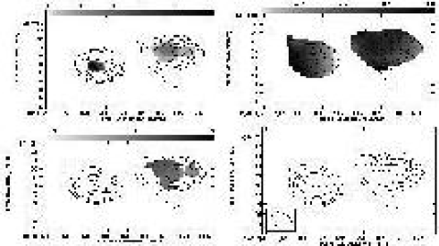
Figure 3: Maps of the radio source 6C0943+39.(a - top left) Map of the depolarisation between 4710 MHz and 1465 MHz. (b - top right) Map of the spectral index between 4710 MHz and 1465 MHz. (c - bottom left) Map of the rotation measure (rad m^-2) between 4710 MHz, 1665 MHz and 1465 MHz. (d - bottom right) Map of the magnetic field direction (degrees).All contours are at $5\sigma$ at 4710 MHz(0.5 mJy beam^-1)x (-1, 1, 2, 4…,1024). Beam size of 2.5” x 1.4”.

In Figures 3 to 29, maps of the radio properties discussed above are presented for all the sources from the 3 samples. Each figure shows the depolarisation map (where the polarisation was detected at all frequencies), the spectral index map, the rotation measure map and the magnetic field direction map (when a rotation measure is detected), if no previously published maps exist. For the three 7C sources, 6C1018+37, 3C65, 3C267 and 3C46 polarisation maps have also been included for both 1.4 GHz and 4.8 GHz as there are no published polarisation maps of these sources. Table 5 contains a listing of published maps for all sources. In all cases only regions from the top end of the grey- scales saturate, as we have always kept the lowest values well inside the grey-scales, to ensure that no information has been lost.

Table 5: Details of previously published maps. TI = total intensity, P = polarisation, S = spectral index & D = depolarisation

Source	Map	Freq.	Ref.
		(GHz)
6C0943+39	P	4.8	?
6C1011+36	P	4.8	?
	TI	1.4	?
6C1129+37	P	4.8	?
	TI	1.4	?
6C1256+36	P	4.8	?
	TI	1.4	?
6C1257+36	P	4.8	?
	TI	1.4	?
3C65	TI	1.4, 4.8	?
3C68.1	P	4.8	?
	TI	1.4	?
3C252	P	4.8	?
3C265	P	4.8	?
3C267	TI	4.8	?
		1.4	?
3C268.1	P	4.8	?
	TI	1.4	?
3C280	P	1.4, 4.8	?
	S, D	1.4, 4.8	?
3C324	TI	4.8	?
	P	1.4	?
4C16.49	P	4.8	?
3C16	TI	4.8	?
	P	1.4	?
3C42	P	4.8	?
3C46	TI	4.8	?
		1.4	?
3C299	P	1.4, 4.8	?
	S, D	1.4, 4.8	?
3C341	P	1.4	?
3C351	TI	4.8	?
	P	1.4	?
3C457	P	1.4	?
4C14.27	P	1.4	?

In order to check the quality of our maps we also used the maximum entropy method implemented in the AIPS task VTESS instead of the CLEAN algorithm. The resulting maps are not significantly different from those produced by the CLEAN algorithm. In fact, VTESS is not necessarily superior to CLEAN in producing accurate maps of extended low surface brightness regions (?).

Depolarisation shadows (regions where the depolarisation is appreciably greater than in the surrounding area) are seen in a few sources, e.g. Figure 19, and may be real features. These were first found by ? in a study of Fornax A. Depolarisation shadows can be caused by the parent galaxy as in the case of 3C324 or by an external galaxy in the foreground of the source, causing a depolarising silhouette (?).

Polarisation angle measurements are ambiguous by $\pm$n$\pi$ and this can introduce ambiguities in the rotation measure. A change of $\pi$ between 1.4 GHz and 5 GHz introduced by the fitting algorithm will cause a change of $\approx$ 80 rad m^-2 in rotation measure. To determine if any strong rotation measure feature is real a plot of the polarisation angle against $\lambda^{2}$, including $n\pi$ ambiguities can be produced. The best fit from AIPS is then overlayed. Any true feature will not show any errors in $n\pi$. This has been done for two sources: 4C16.49 and 6C1256+36. The resulting fits are presented in Figures 30 to 32 and will be discussed in the relevant notes on these sources. The corresponding $\chi^{2}$ values for the fits are tabulated in Table 8. Another test that a feature is real is that a true jump in rotation measure causes depolarisation near the jump but the magnetic field map shows no corresponding jump in the region.

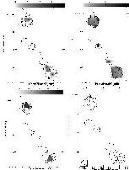
Figure 4: Maps of the radio source 6C1011+36.(a - upper left) Map of the depolarisation between 4535 MHz and 1465 MHz. (b - upper right) Map of the spectral index between 4535 MHz and 1465 MHz. (c - lower right) Map of the magnetic field direction (degrees). (d - lower left)Map of the rotation measure (rad m^-2) between 4710 MHz, 1665 MHz and 1465 MHz. All contours are at $5\sigma$ at 4710 MHz(0.4 mJy beam^-1)x (-1, 1, 2, 4…,1024). Beam size of 3.5” x 3.2”.

3.1 Notes on the individual sources:

3.1.1 Sample A:

6C0943+39:

(Figure 3) No core is detected in the observations, ? detected a core at 8.2 GHz and minimally at 4.8 GHz. Our non-detection is probably due to the different resolution of the data. The value of the rotation measure in the Eastern lobe must be considered with caution as it is based on only a few pixels.

6C1011+36:

(Figure 4) This is a classic double-lobed structure, showing a strong core at both 4.7 GHz and 1.4 GHz with an inverted spectrum.

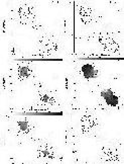
Figure 5: Maps of the radio source 6C1018+37. (a - upper left) 4710 MHz total intensity map with vectors of polarisation overlaid. The contour levels are at $5\sigma$ (100 $\mu$Jy beam^-1)x (-1, 1,2, 4…,1024). 1 arc second corresponds to $1.7\times 10^{-3}{\rm Jybeam}^{-1}$. (b - upper right) 1465 MHz total intensity map with vectors of polarisation overlaid. The contour levels are at $3\sigma$ (0.5 mJy beam^-1)x (-1, 1,2, 4,…,1024). 1 arc second corresponds to $1.7\times 10^{-3}{\rm Jybeam}^{-1}$ (c - middle left) Map of the depolarisation between 4710 MHz and 1465 MHz. (d - middle right) Map of the Spectral Index between 4710 MHz and 1465 MHz. (e - lower right) Map of the magnetic field direction (degrees). (f - lower left) Map of the rotation measure (rad m^-2) between 4710 MHz, 1665 MHz and 1465 MHz. All contours (c-f) are at $5\sigma$ at 4885 MHz (100 $\mu$Jy beam^-1)x (-1, 1, 2, 4…,1024). Beam size of 4” x 4”.

6C1018+37:

(Figure 5) The maps were made with the smaller arrays only at each frequency. In the 1.4 GHz A-array data set the lower lobe was partially resolved out but this was compounded by the high noise, so no feasible combination of the A and B array was possible. To maintain consistency the B-array 4.7 GHz data was also excluded.

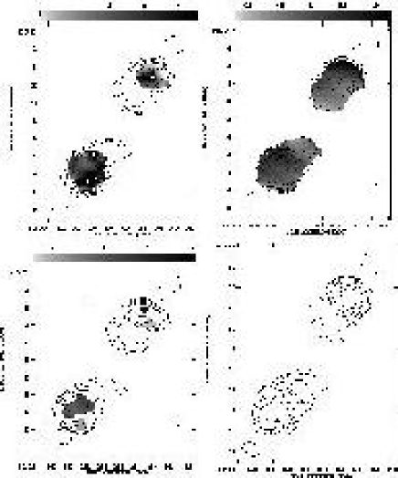
Figure 6: Maps of the radio source 6C1129+37. (a - upper left) Map of the depolarisation between 4710 MHz and 1465 MHz. (b - upper right) Map of the spectral index between 4710 MHz and 1465 MHz. (c - lower right) Map of the magnetic field direction (degrees). (d - lower left) Map of the rotation measure (rad m^-2) between 4710 MHz, 1665 MHz and 1465 MHz. All contours are at $5\sigma$ at 4710 MHz(0.3mJy beam^-1)x (-1, 1, 2, 4…,1024). Beam size of 2.5” x 1.4”.

6C1129+37:

(Figure 6) The SE lobe contains two distinct hotspots. ? found 3 hotspots. Our non-detection is probably due to the different resolutions of the two observations. The source shows distinct regions of very strong depolarisations, however these regions are slightly smaller than the beam size.

6C1256+36:

(Figure 7) The rotation measure map shows distinct changes in the values of the rotation measure. Plot 32 shows that although the jump in RM does not correspond to a jump in depolarisation it is not due to any error in the fitting program.

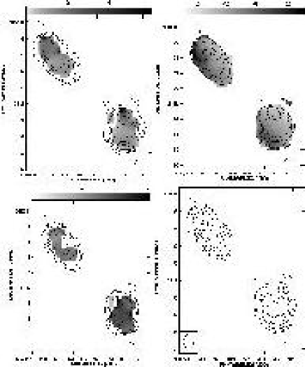
Figure 7: Maps of the radio source 6C1256+36. (a - upper left) Map of the depolarisation between 4710 MHz and 1465 MHz. (b - upper right) Map of the spectral index between 4710 MHz and 1465 MHz. (c - lower right) Map of the magnetic field direction (degrees). (d - lower left)Map of the rotation measure (rad m^-2) between 4710 MHz, 1665 MHz and 1465 MHz. All contours are at $5\sigma$ at 4710 MHz (0.25mJy beam^-1)x (-1, 1, 2, 4…,1024). Beam size of 2.5” x 1.4”.

6C1257+37:

(Figure 8) A core was detected at 4.7 GHz but was absent from the 1.4 GHz data. The high noise level and short observation time meant that the S lobe had very little polarised flux above the noise level, resulting in a reliable value for the rotation measure being found in only a few pixels around the hotspots.

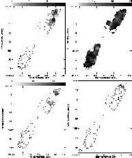
Figure 8: Maps of the radio source 6C1257+37.(a - upper left) Map of the depolarisation between 4710 MHz and 1465 MHz. (b - upper right) Map of the spectral index between 4860 MHz and 1465 MHz. (c - lower right) Map of the magnetic field direction (degrees). (d - lower left) Map of the rotation measure (rad m^-2) between 4710 MHz, 1665 MHz and 1465 MHz. All contours are at $5\sigma$ at 4710 MHz (0.25 mJy beam^-1)x (-1, 1, 2, 4…,1024). Beam size of 2.0” x 1.4”.

7C1745+642:

(Figure 9) This is a highly core dominated source, with the northern lobe appearing faintly. There is an indication of a jet-like structure leading down from the core into the southern, highly extended, off-axis, lobe. The source is a weak core dominated quasar (?).

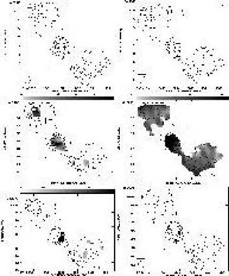
Figure 9: Maps of the radio source 7C1745+642. (a - upper left) 4710 MHz total intensity map with vectors of polarisation overlaid. The contour levels are at $5\sigma$ (0.3mJy beam^-1)x (-1, 1, 2, 4…,1024). 1 arc second corresponds to $1.7\times 10^{-3}{\rm Jybeam}^{-1}$. (b - upper right) 1465 MHz total intensity map with vectors of polarisation overlaid. The contour levels are at $3\sigma$ (0.6 mJy beam^-1)x (-1, 1, 2,, 4…,1024). 1 arc second corresponds to $1.7\times 10^{-3}{\rm Jybeam}^{-1}$ (c - middle left) Map of the depolarisation between 4710 MHz and 1465 MHz. (d - middle right) Map of the Spectral Index between 4710 MHz and 1465 MHz. (e - lower right) Map of the magnetic field direction (degrees). (f - lower left) Map of the rotation measure (rad m^-2) between 4710 MHz, 1665 MHz and 1465 MHz. All contours (c-f) are at $5\sigma$ at 4710 MHz (0.3 mJy beam^-1)x (-1, 1, 2, 4…,1024). Beam size of 1.7” x 1.2”.

7C1801+690:

(Figure 10) This is an asymmetric core dominated quasar (?). The N lobe is very faint and appears to be much closer to the core component than the more extended S lobe. It shows very little polarisation compared to the relatively strong polarisation of the core and S components.

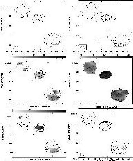
Figure 10: Maps of the radio source 7C1801+690. (a - upper left) 4710 MHz total intensity map with vectors of polarisation overlaid. The contour levels are at $5\sigma$ (0.3 mJy beam^-1)x (-1, 1, 2, 4…, 1024). 1 arc second corresponds to $1.7\times 10^{-3}{\rm Jybeam}^{-1}$. (b - upper right) 1465 MHz total intensity map with vectors of polarisation overlaid. The contour levels are at $3\sigma$ (0.6 mJy beam^-1)x (-1, 1, 2, 4,..,1024). 1 arc second corresponds to $1.7\times 10^{-3}{\rm Jybeam}^{-1}$. (c - middle left) Map of the depolarisation between 4710 MHz and 1465 MHz. (d - middle right) Map of the spectral index between 4710 MHz and 1465 MHz. (e - lower right) Map of the magnetic field direction (degrees). (f - lower left) Map of the rotation measure (rad m^-2) between 4710 MHz, 1665 MHz and 1465 MHz. All contours (c-f) are at $5\sigma$ at 4710 MHz (0.30 mJy beam^-1)x (-1, 1, 2, 4…,1024). Beam size of 2.2” x 1.5”.

7C1813+684:

(Figure 11) This is the faintest of the sources in sample A and is also a quasar (?). The source shows a compact core that is present at all observing frequencies, but it is too faint to detect any reliable polarisation properties.

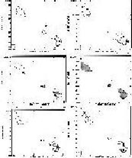
Figure 11: Maps of the radio source 7C1813+684. (a - upper left) 4710 MHz total intensity map with vectors of polarisation overlaid. The contour levels are at $5\sigma$ (0.35 mJy beam^-1)x (-1, 1, 2, 4… ,1024). 1 arc second corresponds to $8.3\times 10^{-4}{\rm Jybeam}^{-1}$. (b - upper right) 1465 MHz total intensity map with vectors of polarisation overlaid. The contour levels are at $3\sigma$ (0.7 mJy beam^-1)x (-1, 1, 2, 4… ,1024). 1 arc second corresponds to $1.7\times 10^{-3}{\rm Jybeam}^{-1}$. (c - middle left) Map of the depolarisation between 4710 MHz and 1465 MHz. (d - middle right) Map of the spectral index between 4710 MHz and 1465 MHz. (e - lower right) Map of the magnetic field direction (degrees). (f - lower left) Map of the rotation measure (rad m^-2) between 4710 MHz, 1665 MHz and 1465 MHz. All contours (c-f) are at $5\sigma$ at 4710 MHz (0.35 mJy beam^-1)x (-1, 1, 2, 4…,1024). Beam size of 2.5” x 2.0”.

3.1.2 Sample B:

3C65:

(Figure 12) The W lobe shows a strong depolarisation shadow that is smaller than the beam size. ? found the source to lie in a cluster which might account for the presence of the depolarisation shadow and the large depolarisation overall.

3C68.1:

(Figure 13) The source is a quasar (?). A core has been detected by ? in deeper observations.

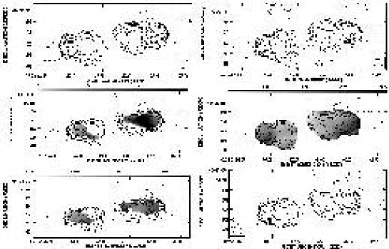
Figure 12: Maps of the radio source 3C65. (a - upper left) 4710 MHz total intensity map with vectors of polarisation overlaid. The contour levels are at $5\sigma$ (0.8 mJy beam^-1)x (-1, 1, 2, 4… ,1024). 1 arc second corresponds to $1.7\times 10^{-2}{\rm Jybeam}^{-1}$. (b - upper right) 1465 MHz total intensity map with vectors of polarisation overlaid. The contour levels are at $3\sigma$ (3.0 mJy beam^-1)x (-1, 1, 2, 4… ,1024). 1 arc second corresponds to $8.3\times 10^{-3}{\rm Jybeam}^{-1}$. (c - middle left) Map of the depolarisation between 4710 MHz and 1465 MHz. (d - middle right) Map of the spectral index between 4710 MHz and 1465 MHz. (e - bottom left) Map of the rotation measure (rad m^-2) between 4710 MHz, 1665 MHz and 1465 MHz. (f - bottom right) Map of the magnetic field direction (degrees). All contours (c-f) are at $5\sigma$ at 4860 MHz(0.8 mJy beam^-1)x (-1, 1, 2, 4…,1024). Beam size of 2.0” x 1.5”.

3C252:

(Figure 14) The SE lobe shows a sharp drop in the polarisation between the 4.7 GHz and 1.4 GHz observations.

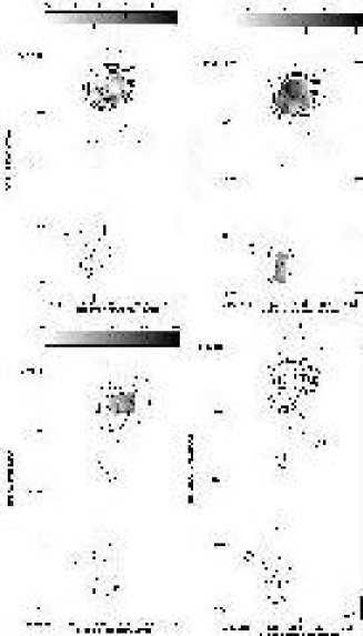
Figure 13: Maps of the radio source 3C68.1. (a - upper left) Map of the depolarisation between 4710 MHz and 1417 MHz. (b - upper right) Map of the spectral index between 4710 MHz and 1417 MHz. (c - lower right) Map of the magnetic field direction (degrees). (d - lower left) Map of the rotation measure (rad m^-2) between 4710 MHz, 1662 MHz and 1417 MHz. All contours are at $5\sigma$ at 4710 MHz (2.0 mJy beam^-1)x (-1, 1, 2, 4…,1024). Beam size of 3.5” x 3.5”.

3C265:

(Figure 15) The NW lobe shows evidence of a compact, bright region with a highly ordered magnetic field which ? show is the primary hotspot at higher resolutions.

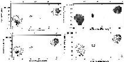
Figure 14: Maps of the radio source 3C252 . (a - top left) Map of the depolarisation between 4710 MHz and 1465 MHz. (b - top right) Map of the spectral index between 4710 MHz and 1465 MHz. (c - bottom left) Map of the rotation measure (rad m^-2) between 4710 MHz, 1665 MHz and 1465 MHz. (d - bottom right) Map of the magnetic field direction (degrees). All contours are at $5\sigma$ at 4710 MHz (0.4 mJy beam^-1)x (-1, 1, 2, 4…,1024). Beam size of 2.0” x 2.5”.

3C267:

(Figure 16) The E lobe is highly extended, reaching to the core position, which can be seen in the 1.4 GHz image. The large depolarisation region in the W lobe coincides with a region of no observed rotation measure. The core is strongly inverted with $\alpha=0.48$

Figure 15: Maps of the radio source 3C265.(a - top left) Map of the depolarisation between 4848 MHz and 1417 MHz. (b - top right) Map of the spectral index between 4848 MHz and 1417 MHz. (c - bottom left) Map of the rotation measure (rad m^-2) between 4848 MHz, 1662 MHz and 1417 MHz. (d - bottom right) Map of the magnetic field direction (degrees) All contours are at $5\sigma$ at 4848 MHz (0.7 mJy beam^-1)x (-1, 1, 2, 4…,1024). Beam size of 3.5” x 3.0”.

3C268.1:

(Figure 17) The average spectral index over the entire source is $\alpha=-0.66$ which is rather flat but taking the 4.8 GHz data from ? and 1.4 GHz data from ? the value is very similar, $\alpha=-0.68$.

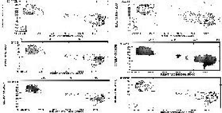
Figure 16: Maps of the radio source 3C267 . (a - upper left) 4848 MHz total intensity map with vectors of polarisation overlaid. The contour levels are at $5\sigma$ (0.8 mJy beam^-1)x (-1, 1, 2, 4… ,1024). 1 arc second corresponds to $8.3\times 10^{-3}{\rm Jybeam}^{-1}$. (b - upper right) 1465 MHz total intensity map with vectors of polarisation overlaid. The contour levels are at $3\sigma$ (1.3 mJy beam^-1)x (-1, 1, 2, 4… ,1024). 1 arc second corresponds to $8.3\times 10^{-3}{\rm Jybeam}^{-1}$. (c - middle left) Map of the depolarisation between 4848 MHz and 1465 MHz. (d - middle right) Map of the spectral index between 4848 MHz and 1465 MHz. (e - bottom left) Map of the rotation measure (rad m^-2) between 4848 MHz, 1665 MHz and 1465 MHz. (f - bottom right) Map of the magnetic field direction (degrees). All contours (c-f)are at $5\sigma$ at 4848 MHz (0.8 mJy beam^-1)x (-1, 1, 2, 4…,1024). Beam size of 2.2” x 2.0”.

3C280:

(Figure 18) The value of the rotation measure and the magnetic field direction in the E lobe must be treated with caution as it is based on only a small region of the entire lobe. The sharp changes in the rotation measure map are not seen in the magnetic field map and the depolarisation map shows a similar structure suggesting that is not due a fitting error.

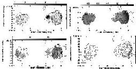
Figure 17: Maps of the radio source 3C268.1.(a - top left) Map of the depolarisation between 4848 MHz and 1417 MHz. (b - top right) Map of the spectral index between 4848 MHz and 1417 MHz. (c - bottom left) Map of the rotation measure (rad m^-2) between 4848 MHz, 1662 MHz and 1417 MHz. (d - bottom right) Map of the magnetic field direction (degrees). All contours are at $5\sigma$ (5.2 mJy beam^-1)x (-1, 1, 2, 4…,1024). Beam size of 4.0” x 3.5”.

3C324:

(Figure 19) The NE lobe shows evidence of a depolarisation shadow. ? found the source to lie in a cluster which may explain the faint shadow.

4C16.49:

(Figure 20) The source is a quasar (?), that shows a strong radio core, jet structure and possibly a small counter-jet. The source is highly asymmetric with the lower lobe almost appearing to connect to the core. It has a very steep spectral index, $\alpha<-1.0$ making it an atypical source. Figures 30 and 31 demonstrates that the sharp changes in the rotation measure map are not due to any fitting errors.

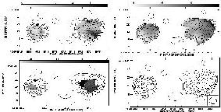
Figure 18: Maps of the radio source 3C280 . (a - top left) Map of the depolarisation between 4848 MHz and 1465 MHz. (b - top right) Map of the spectral index between 4848 MHz and 1465 MHz. (c - bottom left) Map of the rotation measure (rad m^-2) between 4848 MHz, 1665 MHz and 1465 MHz. (d - bottom right) Map of the magnetic field direction (degrees). All contours are at $5\sigma$ at 4848 MHz (0.8 mJy beam^-1)x (-1, 1, 2, 4…,1024). Beam size of 1.6” x 1.6”.

3.1.3 Sample C:

3C16:

(Figure 21) The source shows a strong SW lobe, with a relaxed NE lobe. The SW lobe shows a strong depolarisation feature that is narrower than the beam size. The strong rotation measure feature is evident in the depolarisation map but not the magnetic field map, indicating that it is not an error in the fitting program. No value for the rotation measure was obtained for the NE lobe because the polarisation observed was too weak.

3C42:

(Figure 22) The core was detected at 4.7 GHz but was absent at the lower frequencies. The source has been observed to lie in a small cluster by ?. ? observed that the N hotspot was double but this is not evident in our observations which can be attributed to the differences in the resolutions of the two observations.

3C46:

(Figure 23) The source has a prominent core at 4710 MHz but it is indistinguishable from the extended lobe at 1452 MHz.

3C341:

(Figure 24) The source is a classic double with a resolved jet-like structure running into the SW lobe. The jet is more prominent in the higher frequency observations than at the lower frequencies.

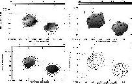
Figure 19: Maps of the radio source 3C324 . (a - top left) Map of the depolarisation between 4848 MHz and 1465 MHz. (b - top right) Map of the spectral index between 4848 MHz and 1465 MHz. (c - bottom left) Map of the rotation measure (rad m^-2) between 4848 MHz, 1665 MHz and 1465 MHz. (d - bottom right) Map of the magnetic field direction (degrees). All contours are at $5\sigma$ at 4848 MHz (1.5 mJy beam^-1)x (-1, 1, 2, 4…,1024). Beam size of 2.2” x 1.6”.

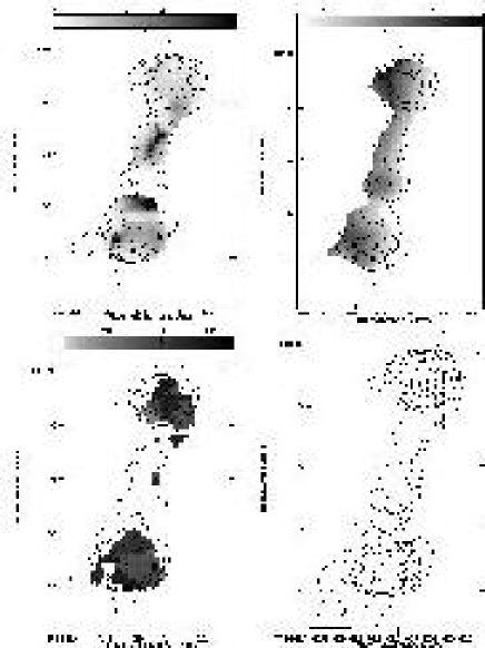
Figure 20: Maps of the radio source 4C16.49. (a - upper left) Map of the depolarisation between 4710 MHz and 1465 MHz. (b - upper right) Map of the spectral index between 4710 MHz and 1465 MHz. (c - lower right) Map of the magnetic field direction (degrees). (d - lower left) Map of the rotation measure (rad m^-2) between 4710 MHz, 1665 MHz and 1465 MHz. All contours are at $5\sigma$ at 4710 MHz (0.8mJy beam^-1)x (-1, 1, 2, 4…,1024). Beam size of 2.2” x 1.8”.

3C351:

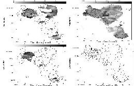
Figure 25: Maps of the radio source 3C351 . (a - upper left) Map of the depolarisation between 4810 MHz and 1452 MHz. (b - upper right) Map of the spectral index between 4810 MHz and 1452 MHz. (c - lower right) Map of the magnetic field direction (degrees). (d - lower left) Map of the rotation measure (rad m^-2) between 4810 MHz, 1502 MHz and 1452 MHz. All contours are at $5\sigma$ at 4810 MHz (1.0mJy beam^-1)x (-1, 1, 2, 4…,1024). Beam size of 4.5” x 4.0”.

(Figure 25) The source is an extended and distorted quasar (?). Both lobes expand out to envelope the core. The NE lobe is highly extended, off-axis and shows two very distinct hotspots. The depolarisation increases towards the more compact SW lobe enforcing the idea that the environment around the SW lobe is denser, stopping the expansion seen in the NE lobe. There is evidence of a rotation measure ridge in the NE hotspots which corresponds to a narrow ridge of depolarisation but there is no corresponding shift in the magnetic field map.

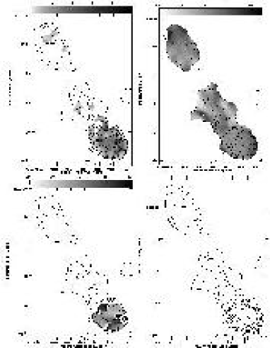
Figure 21: Maps of the radio source 3C16. (a - upper left) Map of the depolarisation between 4710 MHz and 1452 MHz. (b - upper right) Map of the spectral index between 4710 MHz and 1452 MHz. (c - lower right) Map of the magnetic field direction (degrees). (d - lower left) Map of the rotation measure (rad m^-2) between 4885 MHz, 4535 MHz, 1502 MHz and 1452 MHz. All contours are at $5\sigma$ at 4710 MHz (0.40 mJy beam^-1)x (-1, 1, 2, 4…,1024). Beam size of 3.5” x 3.5”.

3C457:

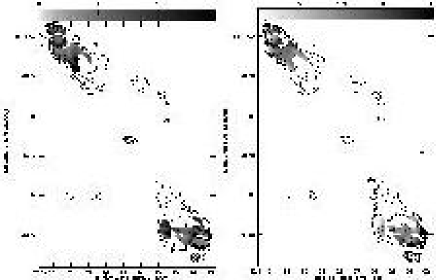
Figure 26: Maps of the radio source 3C457 . (a - top left) Map of the depolarisation between 4710 MHz and 1452 MHz. (b - top right) Map of the spectral index between 4710 MHz and 1452 MHz. All contours are at $5\sigma$ at 4710 MHz (0.3 mJy beam^-1)x (-1, 1, 2, 4…,1024). Beam size of 5.0” x 3.0”.

(Figure 26) The SW lobe shows a prominent double hotspot. The small compact object just south of the SW hotspots is most likely an unrelated background object. The inverted core was observed to be present at all frequencies. This source has no rotation measure map or magnetic field measure map as we were unable to remove all n$\pi$ ambiguities from this source. This was due to the small separation of observing frequencies around 1.4 GHz and 5 GHz, see Section 2.3

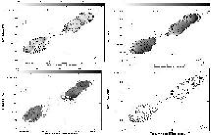
Figure 22: Maps of the radio source 3C42 . (a - upper left) Map of the depolarisation between 4710 MHz and 1452 MHz. (b - upper right) Map of the spectral index between 4710 MHz and 1465 MHz. (c - lower right) Map of the magnetic field direction (degrees). (d - lower left) Map of the rotation measure (rad m^-2) between 4885 MHz, 4535 MHz, 1502 MHz and 1452 MHz. All contours are at $5\sigma$ at 4710 MHz (1.0 mJy beam^-1)x (-1, 1, 2, 4…,1024). Beam size of 2.5” x 1.8”.

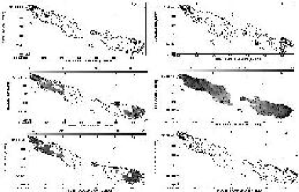
Figure 23: Maps of the radio source 3C46. (a - upper left) 4710MHz total intensity map with vectors of polarisation overlaid. The contour levels are at $5\sigma$ (0.2 5mJy beam^-1)x (-1, 1, 2, 4…, 1024). 1 arc second corresponds to $1.7\times 10^{-3}{\rm Jybeam}^{-1}$. (b - upper right) 1452MHz total intensity map with vectors of polarisation overlaid. The contour levels are at $3\sigma$ (1.0 mJy beam^-1)x (-1, 1, 2, 4,..,1024). 1 arc second corresponds to $5.5\times 10^{-4}{\rm Jybeam}^{-1}$.(c - middle right) Map of the depolarisation between 4710 MHz and 1452 MHz. (d - middle left) Map of the spectral index between 4710 MHz and 1452 MHz. (e - bottom right) Map of the rotation measure (rad m^-2) between 4885 MHz, 4535 MHz, 1502 MHz and 1452 MHz. (f - bottom left) Map of the magnetic field direction (degrees). All contours (c- f) are at $5\sigma$ at 4710 MHz (0.25mJy beam^-1)x (-1, 1, 2, 4…,1024). Beam size of 4.5” x 3.0”.

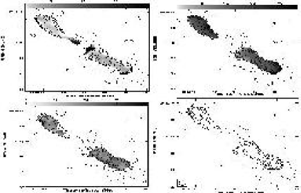
Figure 24: Maps of the radio source 3C341 . (a - upper left) Map of the depolarisation between 4710 MHz and 1452 MHz. (b - upper right) Map of the spectral index between 4710 MHz and 1452 MHz. (c - lower right) Map of the magnetic field direction (degrees). (d - lower left) Map of the rotation measure (rad m^-2) between 4885 MHz, 4535 MHz, 1502 MHz and 1452 MHz. All contours are at $5\sigma$ at 4710 MHz (0.7 mJy beam^-1)x (-1, 1, 2, 4…,1024). Beam size of 4.0” x 4.0”.

3C299:

(Figure 27) The source is the least luminous in all of the samples. The source shows a large change in rotation measure between the lobes but the difference is probably due to the small number of pixels with rotation measure information in the NE lobe.

4C14.27:

(Figure 29) There is no core detected at any frequency even in a better quality map by ?.

4 Discussion

Table 6: Properties of the sample A radio source components. Errors are 5% or less unless stated otherwise. The spectral indices are the mean values for each component, calculated between approximately 4800 MHz and 1465 MHz. The depolarisation measures are the mean values of the ratio of the fractional polarisation between approximately 4800 MHz and 1465 MHz for each component. The rotation measures are the mean values between approximately 4710 MHz, 1665 MHz and 1465 MHz and are quoted in the observer’s frame of reference. The Faraday dispersion, $\Delta$, is given in Equation 5. $\sigma_{RM}$ is the rms in the rotation measure. All mean values take into account pixels above 5$\sigma_{rms}$ at 4.7 GHz and above 3$\sigma_{rms}$ at 1.4 GHz.

Source	Component	Total	Percentage	Total	Percentage	Rotation	Spectral	Depolarisation	Average	$\sigma_{RM}$
		Flux	Polarisation	Flux	Polarisation	Measure	Index	Measure	$\Delta$
		4710 MHz	4710 MHz	1465 MHz	1465 MHz	RM	$\alpha$	$DM^{4.8}_{1.4}$
		(mJy)	%	(mJy)	%	(rad m-2)			(rad m-2)	(rad m-2)
$6C0943+37$	W	31.0	11.8	71.7	5.4	1.6 $\pm 2$	-0.72	2.19	15.01	16.1
	E	42.0	2.7	136.4	0.7	-19.1 $\pm 6$	-1.01	3.86	19.7	101.4
$6C1011+36$	N	44.3	7.8	119.6	5.1	30.8 $\pm 5$	-0.88	1.53	11.1	12.8
	S	18.7	12.2	50.9	11.5	12.6 $\pm 4$	-0.89	1.06	4.1	10.1
	Core	3.22	-	0.7 $\pm 0.5$	-	-	1.35	-	-	-
$6C1018+37$	NE	46.4	10.0	125.8	8.1	0.85$\pm 3$	-0.85	1.23	7.71	6.1
	SW	28.7	7.0	76.3	2.9	11.2 $\pm 2$	-0.84	2.41	15.9	2.9
	Core	0.63 $\pm 0.2$	-	-	-	-	-	-	-	-
$6C1129+37$	NW	46.5	7.3	129.1	2.9	-19.3 $\pm 4$	-0.85	2.51	16.3	54.0
	SE	73.2	16.3	215.0	3.2	0.08 $\pm 3$	-0.90	5.09	21.61	22.0
$6C1256+36$	NE	57.8	10.4	148.9	7.7	5.9 $\pm 3$	-0.79	1.35	9.3	21.8
	SW	101.4	8.9	288.5	8.8	15.4 $\pm 3$	-0.87	1.01	1.7	14.0
$6C1257+36$	NW	43.5	17.0	102.2	13.4	-115.3 $\pm 9$	-0.71	1.27	8.3	10.0
	SE	20.5	9.8	73.0	5.2	-115.6 $\pm 10$	-1.06	1.88	13.5	16.0
	Core	0.29 $\pm 0.08$	-	-	-	-	-	-	-	-
$7C1745+642$	N	23.5	9.6	64.5	5.2	-	-0.86	1.85	13.3	-
	Core	84.1	4.9	69.4	2.9	65.4 $\pm 4$	0.16 $\pm 0.1$	1.69	12.3	20.9
	S	33.8	8.6	98.5	9.5	12.8 $\pm 3$	-0.91	0.91	-	3.1
$7C1801+690$	N	8.8 $\pm 3$	3.0	28.2	2.7	44.8 $\pm 3$	-0.97	1.11	5.5	16.0
	Core	79.1	1.8	78.4	4.0	30.3 $\pm 3$	0.007	0.45	-	1.80
	S	28.7	10.0	75.8	7.2	20.8$\pm 2$	-0.81	1.39	9.7	10.0
$7C1813+684$	NE	15.0	7.7	44.8	9.5	13.9$\pm 3$	-0.92	0.81	-	85.0
	SW	30.2	8.4	78.1	7.4	-68.4$\pm 7$	-0.79	1.14	6.1	41.7
	Core	3.32	-	2.65	-	-	0.19 $\pm 0.1$	-	-	-

Table 10 shows the average of the various observed properties of each of the samples. The average was calculated by taking the properties of both lobes in each source, averaging them together and then averaging these values over the sample. Differential properties, e.g. the difference of rotation measure, dRM, were calculated by taking the difference of the respective property between the two lobes of each source and then averaging these values over the entire sample. These sample-averaged properties give very simple indicators of trends between samples and hence reveal the strongest correlations of source properties with redshift and/or radio power. We will present a more extensive statistical analysis of these correlations in a forthcoming paper.

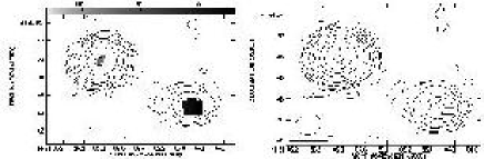
Figure 27: Maps of the radio source 3C299 . (a - left) Map of the rotation measure (rad m^-2) between 4770 MHz, 1502 MHz and 1452 MHz. (b - right) Map of the magnetic field direction (degrees). All contours are at $5\sigma$ at 4770 MHz (0.7 mJy beam^-1)x (-1, 1, 2, 4…,1024). Beam size of 2.5” x 2.0”.

4.1 The location of the Faraday screen

The observed rotation measure, RM, and degree of polarisation in a source may be caused by plasma either inside the radio source itself (internal depolarisation) or by a Faraday screen in between the source and the observer (external depolarisation). In the latter case the screen may be local to the radio source or within our own Galaxy, or both. Only in the case of an external Faraday screen local to the radio source do our measurements contain information on the source environment.

The average RM we observe in our sources is consistent with a Galactic origin (?). This is also consistent with the absence of any significant differences of RM between our samples (see Table 10). However, we observe large variations of RM within individual lobes on small angular scales. These are probably caused by a Faraday screen local to the source (?) and therefore must be corrected for the source redshift by multiplying dRM and $\sigma_{RM}$ by a factor $(1+z)^{2}$ to allow a valid comparison between sources. The variation of RM on large angular scales (10s of arcseconds), i.e. between the two lobes of a source, dRM, may still be somewhat influenced by the Galactic Faraday screen. Nevertheless, the large variations of RM found on arcsecond scales measured by $\sigma_{RM}$ suggest an origin local to the source.

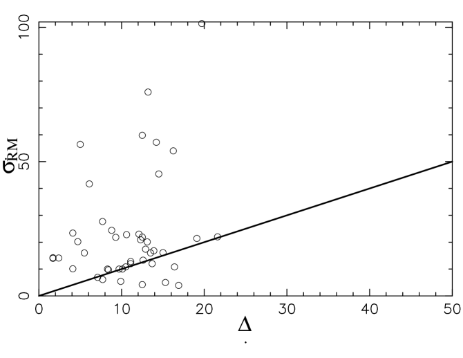
Figure 28: Plot of the Faraday dispersion, $\Delta$ against the rms of the rotation measures for each source.

Figure 29: Maps of the radio source 4C14.27 . (a - top left) Map of the depolarisation between 4710 MHz and 1452 MHz. (b - top right) Map of the spectral index between 4710 MHz and 1452 MHz. (c - bottom left) Map of the rotation measure (rad m^-2) between 4885 MHz, 4535 MHz, 1502 MHz and 1452 MHz. (d - bottom right) Map of the magnetic field direction (degrees). All contours are at $5\sigma$ at 4710 MHz (0.4 mJy beam^-1)x (-1, 1, 2, 4…,1024). Beam size of 2.5” x 2.0”.

The observed degree of depolarisation in a source depends on the distribution of the Faraday depths covered by the projected area of the telescope beam, i.e. the variation of RM on the smallest angular scales. We therefore assume that the depolarisation in our sources is caused by plasma local to the sources. If the depolarisation is caused by a local but external Faraday screen and the distribution of Faraday depths in this screen is Gaussian with standard deviation $\Delta$, then (e.g. ?)

$$m_{\lambda}=m_{0}\exp\left\{-2\Delta^{2}\left[\lambda/\left(1+z\right)\right]^{4}\right\},$$ (4)

where $m_{\lambda}$ is the percentage polarisation at observed wavelength $\lambda$ and $m_{0}$ is the initial percentage polarisation before any depolarisation. Since we measure $m_{\lambda}$ at two observing frequencies (1.4 GHz and 4.8 GHz), we can solve equation (4) for $\Delta$ as a function of the depolarisation measure,

$$\centering\Delta=\sqrt{\frac{(1+z)^{4}lnDM^{4.8}_{1.4}}{2(\lambda_{1.4}^{4}-\lambda_{4.8}^{4})}}{\rm\,rad\,m}^{-2}.\@add@centering$$ (5)

We can now, for each source, compare the value of $\Delta$ as derived from the measured depolarisation with the observed rms of the rotation measure. If the Faraday dispersion is less than the rms of the rotation measure, then our observations are consistent with an external Faraday screen (?).

Figure 28 displays the Faraday dispersion, $\Delta$, for each lobe of the sources against the rms of the rotation measures observed. It is evident from the plot that the value of $\sigma_{RM}>\Delta$ for most components. There are a few sources where this is not the case. However, these components belong to sources where the depolarisation or rotation measure is only determined reliably for a few pixels so an accurate value is not obtainable for $\sigma_{RM}$ or $\Delta$. There is little correlation between $\Delta$ and $\sigma_{RM}$. This is a strong indicator that the Faraday medium responsible for variations of RM on small angular scales, and thus for the polarisation properties of our sources, is consistent with being external but local to the sources.

Table 7: As Table 6 but for sample B.

Source	Component	Total	Percentage	Total	Percentage	Rotation	Spectral	Depolarisation	Average	$\sigma_{RM}$
		Flux	Polarisation	Flux	Polarisation	Measure	Index	Measure	$\Delta$
		4790 MHz	4790 MHz	1465 MHz	1465 MHz	RM	$\alpha$	$DM_{1.4}^{4.8}$
		(mJy)	%	(mJy)	%	(rad m-2)			(rad m-2)	(rad m-2)
$3C65$	W	524.0	19.3	1683.1	5.4	-82.6 $\pm 7$	-1.0	3.57	19.1	21.4
	E	240.9	9.2	800.4	7.2	-86.1 $\pm 6$	-1.03	1.28	8.4	9.7
$3C252$	NW	178.7	6.4	592.2	5.9	15.7 $\pm 6$	-1.0	1.08	4.7	20.2
	SE	80.0	14.1	300.5	6.8	58.5 $\pm 6$	-1.1	2.07	14.5	45.4
	Core	1.98	-	1.33	-	-	0.33	-	-	-
$3C267$	E	184.0	8.9	745.7	6.8	-9.6 $\pm 3$	-1.17	1.31	8.8	24.4
	Core	1.87 $\pm 1$	-	1.05 $\pm 2$	-	-	0.48	-	-	-
	W	479.2	3.5	1294.6	3.3	-21.5$\pm 3$	-0.83	1.06	4.1	23.4
$3C280$	E	326.0	8.0	1219.2	4.4	-37.7$\pm 8$	-1.01	1.82	13.1	20.1
	W	1289.2	10.0	3191.6	6.5	-7.5 $\pm 4$	-0.76	1.54	11.1	1.5
$3C324$	NE	432.6	9.3	1525.2	5.6	22.1 $\pm 4$	-1.05	1.66	12.1	23.0
	SW	166.0	7.8	651.8	4.0	43.0 $\pm 5$	-1.14	1.95	13.9	16.8
$4C16.49$	N	107.2	8.3	307.2	13.0	-4.3 $\pm 5$	-0.88	0.64	-	56.4
	Jet	8.5 $\pm 4$	14.5	45.9	7.2	30.1 $\pm 4$	-1.41	2.01	14.2	57.2
	Core	9.64 $\pm 2$	2.7	58.2	3.5	-	-1.50	0.77	-	-
	S	142.3	7.0	695.3	6.4	0.9 $\pm 3$	-1.32	1.09	5.0	56.4
$3C68.1$	N	667.2	8.6	1767.4	7.0	-26.6$\pm 5$	-0.82	1.23	7.7	27.7
	S	36.8	11.4	134.6	6.6	57.9 $\pm 2$	-1.08	1.73	12.5	59.8
$3C265$	NW	224.0	10.0	478.7	5.8	42.2 $\pm 6$	-0.62	1.72	12.5	21.9
	SE	318.9	6.2	835.0	4.2	32.8$\pm 3$	-0.78	1.48	10.6	22.8
$3C268.1$	E	262.3	5.0	816.4	3.4	21.7 $\pm 5$	-0.92	1.47	10.5	10.8
	W	2296.6	4.7	4699.0	2.7	26.8 $\pm 6$	-0.58	1.74	12.6	13.3

4.2 Trends with redshift and radio power

4.2.1 Spectral index

We found no significant correlation between spectral index and redshift or radio power as suggested by others (???), which used much larger samples. This suggests the trend may be present but because of the fact that our sample is small we do not find any significant trend. However there are trends found with the difference in spectral index between the two lobes. Sample B shows a larger average difference in the spectral indices between the two lobes of a given source than the other samples (Sample A: 2.5$\sigma$, sample C: 3.3$\sigma$). Sample B contains the sources with the highest radio power and so we find that in our samples the difference in spectral index increases with radio power rather than with redshift. The trend of the difference in the spectral index between the two lobes may be related to the extra luminosity of the 3CRR hotspots compared to the 6C/7C hotspots (see Section 2.2). On average we find that the hotspots of our sources have shallower spectral indices. The average spectral index integrated over the entire sources will therefore depend on the fraction of emission from the hotspots compared to the extended lobe, thus creating the observed trend.

Figure 30: A plot of the polarisation angle against $\lambda^{2}$, allowing for n$\pi$, for the northern lobe of 4C16.49 with the dashed lines showing the best fit models. All n$\pi$ solutions for the 5 GHz data are considered and plotted. Data for two small regions, one on each side of the jump are plotted with o indicating one side of the jump and x the other. Table 8 show the $\chi^{2}$ values for each fit. The jump plotted lies SW of the central intensity contour.

Table 8: Reduced $\chi^{2}$ values for the rotation measure fits for Figures 30 to 32.

Source	Lobe	n=-1	n=0	n=1	Symbol
6C1256+36	S	382.	51.	1.91	x
		981.6	1.23	976.5	o
4C16.49	N	1.6	669.	2917.	o
		2772.	90.1	1.7	x
4C16.49	S	151.9	0.9	62.	o
		45.4	0.4	34.8	x

Figure 31: As Figure 30 but for 4C16.49 south lobe.Data for two small regions, one on each side of the jump are plotted. These regions lie either side of the jump south of the peak intensity contour.

Figure 32: As Figure 30 but for 6C1256+36 south lobe.Data for two small regions, one on each side of the jump are plotted.

4.2.2 Rotation measure

As mentioned above, we find no significant difference in the average RM between our samples. Similarly, there is no statistically significant trend of the difference of RM between the two lobes of each source with redshift or radio power. This is consistent with a Galactic origin of the RM properties of the sources on large scales. On small angular scales the variation of RM as measured by its rms variation $\sigma_{RM}$ shows a significant trend between the low redshift sample (C) and the high redshift samples (A: 2.6$\sigma$, B: 3.3$\sigma$). The exclusion of 3C457 due to $n\pi$-ambiguities in the rotation measure (see section 2.3) from the rotation measure averages could bias the sample C results towards a small value of $\sigma_{RM}$. In principle, similar ambiguities could also affect other sources in sample C. However, as stated above we find the rotation measure to vary smoothly across the other sources in this sample. The exclusion of one source will not remove the trend we find here. There is no significant difference between the low power sample A compared with the high power sample B. This suggests that at least the range of rotation measures on small angular scales in a source does depend on the source redshift and not the source radio power. In a recent study by ? rotation measure was also found to be independent of source luminosity and size but dependent on the redshift of the source.

Figure 33: Average depolarisation against projected linear size (kpc) for all 3 samples. Symbols as in Figure 1. Figure (a) assumes $H_{o}=50$ kms^-1Mpc^-1, and $\Omega_{m}=0.5$, $\Omega_{\Lambda}=0$. Figure (b) assumes $H_{o}=50$ kms^-1Mpc^-1, and $\Omega_{m}=0.35$, $\Omega_{\Lambda}=0.65$.

4.2.3 Percentage polarisation

The flux observed from both lobes of all sources was found to be polarised at levels greater than 1%, the only exceptions being 6C0943+39 and 3C299. At lower redshifts the polarisation exhibits the largest range from 0.8% in 3C299 to 28.0% in 3C341. This range is not evident in either of the other two samples. Statistically the sources at low redshift (sample C) are slightly more polarised than those at high redshift both at 1.4 GHz (sample A: 2.1$\sigma$, sample B: 2.3$\sigma$) but at 4.8 GHz there is no significant difference. There is no trend observed comparing the low radio power sources (sample A) with the high power objects (sample B). This suggests that percentage polarisation decreases for increasing redshift but is less dependent on radio power.

So far we considered percentage polarisations measured in the observing frame. We argue in section 4.1 that variations of the rotation measure on small angular scales which determine the degree of polarisation are caused in Faraday screens local to the sources. The trend with redshift may therefore simply reflect the different shifts of the observing frequency in the source restframe for sources at low and high redshift. Using Burn’s law in the form of equations (4) and (5) we can determine for each source the percentage polarisation expected to be observable at a frequency corresponding to a wavelength of 5 cm in its restframe. The results for individual sources are presented in Table 11 and the sample averages are summarised in Table 12. Again sources at low redshift (sample C) are slightly more polarised than sources at high redshift but only sample B (2.1$\sigma$) shows a result that is marginally significant. As before, there is no trend with radio power, indicating that the trend with redshift, although weak is dominant. This is not caused by pure Doppler shifts of the observing frequencies.

Table 9: As Table 6 but for sample C. Rotation measure is between 4800, 4500, 1502 and 1450

Source	Component	Total	Percentage	Total	Percentage	Rotation	Spectral	Depolarisation	Average	$\sigma_{RM}$
		Flux	Polarisation	Flux	Polarisation	Measure	Index	Measure	$\Delta$
		4710 MHz	4710 MHz	1452 MHz	1452 MHz	RM	$\alpha$	$DM_{1.4}^{4.8}$
		(mJy)	%	(mJy)	%	(rad m-2)			(rad m-2)	(rad m-2)
$3C42$	NW	353.9	12.5	999.7	12.3	-2.4$\pm 5$	-0.87	1.02	2.4	14.1
	SE	450.6	7.5	1266.3	7.4	5.0$\pm 5$	-0.86	1.01	1.7	14.2
$4C14.27$	NW	107.0	12.4	368.2	8.8	-13.0$\pm 4$	-1.06	1.41	9.9	5.4
	SE	124.8	9.6	489.3	9.3	-17.3 $\pm 5$	-1.17	1.03	2.9	4.8
$3C46$	NE	162.7	16.2	488.0	12.8	-4.8 $\pm 5$	-0.94	1.27	16.9	3.9
	SW	173.7	13.7	506.4	12.0	-2.9 $\pm 1$	-0.91	1.14	12.5	4.2
	Core	2.54	-	7.94	-	-	-0.97	-	-	-
$3C457$	NE	208.6	15.8	692.0	15.7	-	-1.02	1.01	-	-
	SW	290.5	11.9	898.9	10.0	-	-0.94	1.19	-	-
	Core	3.03	-	2.63	-	-	0.12	-	-	-
$3C351$	NE	971.7	6.8	2327.9	8.1	1.00 $\pm 5$	-0.73	0.84	-	13.0
	Diffuse	122.2	26.4	421.3	13.7	-8.7 $\pm 1$	-1.03	1.93	13.7	12.0
	Core	18.3	18.6	46.2	8.2	-0.53$\pm 2$	-0.77	2.27	15.3	5.0
	SW	77.1	22.8	235.7	8.9	4.4 $\pm 3$	-0.93	2.56	16.4	10.8
$3C341$	NE	123.8	28.0	336.4	19.6	20.3 $\pm 5$	-0.85	1.43	10.1	10.0
	SW	265.9	26.4	862.6	17.2	18.2 $\pm 5$	-1.0	1.53	11.1	12.0
$3C299$	NE	876.5	0.79$\pm 0.5$	2592.4	0.43 $\pm 0.3$	-126.3 $\pm 8$	-0.93	1.84	13.2	75.9
	SW	53.7	3.1	122.6	2.6	16.0 $\pm 5$	-0.71	1.19	7.10	6.9
$3C16$	NE	22.1 $\pm 3$	10.8	60.9	4.9	-	-0.87	2.2	15.0	-
	SW	484.9	14.7	1510.9	8.2	-4.3 $\pm 3$	-0.97	1.79	12.9	17.4

4.2.4 Depolarisation

Comparing the average depolarisation of individual samples with each other we find only very weak trends with redshift or radio power. When the samples are averaged together we find a trend in depolarisation with redshift but none with radio power. Samples A+C (low radio power) are statistically identical to sample B (high radio power), suggesting that there is no trend with radio power in our sources. By considering the averaged depolarisation of samples A+B (high redshift) compared with that of sample C (low redshift) there is a weak trend with redshift which is echoed in the dDM values. However both results are not significant. This may confirm the results of ?: redshift is the dominant factor compared to radio power in determining the depolarisation properties of a source.

Table 10: Mean properties of the sources averaged over each sample with the associated error. Differential properties (dDM,d$\alpha$,dRM) are derived by taking the difference of the respective property between the two lobes of each source and then averaging this difference over each sample, dRM is in the source frame.$\sigma_{RM}$ is the rms of the RM over the source, in the source reference frame. Properties in italics are in the source frame of reference.

Property	sample	sample	sample	sample	sample
	A	B	C	A+B	A+C
Average z	1.06$\pm 0.04$	1.11$\pm 0.05$	0.41 $\pm 0.01$	1.08 $\pm 0.03$	0.75 $\pm 0.08$
Average P151	$(1.02\pm 0.06)\times 10^{27}$	$(1.01\pm 0.07)\times 10^{28}$	$(8.02\pm 0.40)\times 10^{26}$	$(5.57\pm 1.16)\times 10^{27}$	$(8.97\pm 0.47)\times 10^{26}$
Average D	220.34$\pm 46.40$	262.69$\pm 55.41$	399.57 $\pm 122.50$	241.51 $\pm 35.43$	304.69 $\pm 64.50$
Average DM	1.82 $\pm 0.32$	1.61$\pm 0.13$	1.42 $\pm 0.12$	1.71 $\pm 0.17$	1.63 $\pm 0.18$
dDM	0.93 $\pm 0.26$	0.61 $\pm 0.22$	0.43 $\pm 0.18$	0.77$\pm 0.17$	0.69 $\pm 0.17$
Average $\alpha$	-0.87 $\pm 0.01$	-0.92 $\pm 0.06$	-0.94 $\pm 0.03$	-0.90$\pm 0.03$	-0.90 $\pm 0.02$
d$\alpha$	0.13 $\pm 0.04$	0.23 $\pm 0.04$	0.10 $\pm 0.03$	0.18$\pm 0.03$	0.12 $\pm 0.02$
Average PF1.4	6.29$\pm 0.86$	5.88$\pm 0.64$	9.89 $\pm 1.75$	6.08 $\pm 0.52$	7.98 $\pm 1.01$
Average PF4.8	8.91 $\pm 1.03$	8.76$\pm 0.89$	13.31 $\pm 2.48$	8.83 $\pm 0.66$	10.98 $\pm 1.36$
Average RM	29.03 $\pm 12.81$	26.41 $\pm 7.74$	16.24 $\pm 8.33$	27.64$\pm 7.05$	23.55 $\pm 8.07$
dRM	97.85 $\pm 36.41$	115.96 $\pm 42.81$	50.77$\pm 43.29$	107.44$\pm 27.62$	77.68 $\pm 27.54$
$\sigma_{RM}$	115.62 $\pm 33.43$	122.94 $\pm 28.48$	29.45 $\pm 9.98$	119.49 $\pm 21.11$	78.69 $\pm 22.36$

Analogous to the discussion above on percentage polarisation, the cosmological Doppler shifts of the observing frequencies influence the trend of DM with redshift, and in fact the true trend is stronger than that naively observed. To demonstrate this we use equation (5) to derive the standard deviation of Faraday depths, $\Delta$, for each source. By setting $z=1$ we then rescale all the depolarisations DM${}^{4.8}_{1.4}$ to the same redshift. This allows all 3 samples to be compared without any bias due to pure redshift effects (see Tables 11 and 12). If there was no intrinsic difference between the high-redshift and low-redshift samples then we would expect these values to be consistent with each other. This is evidently not the case. The high redshift samples are, on average significantly more depolarised (sample A: 2.2$\sigma$, sample B: 3.2$\sigma$) than their low-redshift counterparts (sample C). Comparing sample A with sample B we find no trend with radio power. However, a note of caution must be issued as the corrections applied use Burn’s law and may actually be too large. Considering the precorrected and the corrected values together it is obvious that there is a connection between redshift and depolarisation but there is no significant trend of depolarisation with radio power. There is also a connection between the difference in the depolarisation, dDM, and the redshift of the source, but no significant trend of the difference in the depolarisation with the radio power of the source. As noted in Section 2.3 regions with signal-to-noise $<3\sigma$ were blanked in the map production. In individual sources blanking of low S/N regions in the polarisation maps will cause the measured depolarisation to be underestimated. Sources in sample A are more affected by this problem than objects in the other samples. Therefore we probably underestimate the average depolarisation in sample A implying that the trend with redshift could be even stronger than our findings suggest.

The trends of percentage polarisation and of depolarisation with redshift are probably related in the sense that a lower degree of depolarisation at low redshift also leads to a higher observed degree of polarisation. Clearly a variation of the initial polarisation, $m_{0}$, with redshift would lead to variations of the observed $m_{\lambda}$ independent of the properties of any external Faraday screen. Therefore both trends could also be caused by a significantly higher level of $m_{0}$ of the sources at low redshift (sample C). Using equation (4) we find $m_{0}=9.3\pm 1.1$ for sample A, $m_{0}=9.1\pm 1.0$ for sample B and $m_{0}=13.5\pm 2.5$ for sample C. The uncertainties associated with the use of Burn’s law in extrapolating from our observations to $\lambda=0$ are large. There is no difference between average initial polarisation of sources in samples A and B. The difference found for $m_{0}$ at low redshift (sample C) compared to high redshift (samples A and B) is small compared to the difference found for the depolarisation comparing the same samples. This suggests that the differences in percentage polarisation and depolarisation are due to variation with redshift of the Faraday screens local to the sources rather than to differences in the initial degree of polarisation. However note, that the variation of $m_{0}$ is not significantly smaller than the trend of percentage polarisation with redshift.

Table 11: Recalculated average depolarisation and dDM for each source if it was located at z=1 and average percentage polarisation of all sources if it was emitted at 5cm in the rest frame.

Source	z	$\Delta_{z}$	DMz=1	dDMz=1	Polarisation
					$\lambda_{rest}=5cm$
6C0943+37	1.04	74.12	3.31	1.98	3.1
6C1018+37	0.81	42.95	1.49	0.52	8.32
6C1011+36	1.04	36.11	1.33	0.66	5.63
6C1129+37	1.06	83.07	4.49	3.43	3.09
6C1256+36	1.07	29.53	1.21	0.40	8.26
6C1257+36	1.00	45.51	1.58	0.61	9.39
7C1801+690	1.27	41.24	1.45	0.54	3.33
7C1813+684	1.03	6.96	1.01	0.25	8.47
7C1745+642	1.23	47.81	1.65	1.36	7.32
3C65	1.18	75.33	3.50	4.61	6.26
3C252	1.11	50.66	1.76	1.36	6.36
3C267	1.14	32.34	1.26	0.35	5.04
3C280	1.00	48.79	1.68	0.28	5.48
3C324	1.21	54.34	2.42	0.58	4.74
3C265	0.81	35.56	1.37	0.14	5.05
3C268.1	0.97	42.13	1.57	0.25	3.07
3C68.1	1.24	45.11	1.85	0.98	10.2
4C16.49	1.29	31.04	1.23	0.47	6.76
3C42	0.40	4.59	1.00	0.01	9.85
4C14.27	0.39	14.34	1.05	0.08	9.08
3C46	0.44	15.06	1.05	0.03	12.45
3C457	0.43	10.50	1.03	0.04	12.88
3C351	0.37	23.82	1.14	0.15	8.59
3C341	0.45	21.91	1.11	0.02	18.57
3C16	0.41	27.54	1.19	0.06	6.64
3C299	0.37	20.20	1.10	0.1	1.52

Burn’s law predicts a steep decrease of percentage polarisation with increasing observing frequency. Although the decrease may well be ‘softened’ by geometrical and other effects in more realistic source models (?), the value of DM may be small for sources in which our observing frequencies are lower than the frequency at which strong depolarisation occurs. For such sources we expect to measure a low value of DM associated with a low percentage polarisation. ? show that one of our sources, 3C299 (sample C), is strongly depolarised between 1.6 GHz and 8.4 GHz with almost all of the depolarisation taking place between 4.8 GHz and 8.4 GHz. We measure only a very low percentage polarisation for this source and the average value of DM${}^{4.8}_{1.4}=1.5$ is also lower than DM${}^{8.4}_{1.6}\sim 4$ as measured by ?. If many of our sources at low redshift were affected by strong depolarisation at frequencies higher than 4.8 GHz, then this may cause the trend of DM with redshift noted above. The absence of any other sources with very low degrees of polarisation combined with a low value for DM, at least in the low redshift sample C, argues against this bias. In fact, ? show that our sources 3C42, 3C46, 3C68.1, 3C265, 3C267, 3C324 and 3C341 depolarise strongly only at frequencies lower than our observing frequencies. 3C16, 3C65, 3C252, 3C268.1 and 3C280 do depolarise strongly between 1.4 GHz and 4.8 GHz. In all the sources mentioned in the ? none have strong depolarisation at frequencies higher than 4.8 GHz. There is no information for 4C14.27, 4C16.49, 3C351, 3C299 and 3C457. Those sources which do depolarise strongly between our observing frequencies, 1.4 and 4.8 GHz, could in principle have inaccurate values of the rotation measure because of this. However, the pixels containing most depolarised regions of the source are likely to have been blanked because of insufficient signal–to–noise in their polarisation at 1.4 GHz; the rotation measure is determined from the unblanked (less depolarised) regions of the source, and will therefore be reliable.

Table 12: Average DM and dDM now shifted so that all the measurements are taken at z=1. Average polarisation of all the sources, shifted to a common rest frame wavelength of 5cm using Equation 5

Property	sample	sample	sample	sample	sample
	A	B	C	A+B	A+C
Average DMz=1	1.95 $\pm 0.39$	1.85$\pm 0.24$	1.08 $\pm 0.02$	1.90 $\pm 0.22$	1.54 $\pm 0.23$
dDMz=1	1.08 $\pm 0.34$	1.00 $\pm 0.47$	0.06 $\pm 0.02$	1.04$\pm 0.28$	0.60 $\pm 0.22$
PF${}_{\lambda_{rest}=5cm}$	6.32 $\pm 0.86$	5.88$\pm 0.65$	9.82 $\pm 1.85$	6.10 $\pm 0.53$	7.97 $\pm 1.04$

???? find an anti-correlation of depolarisation with linear size. Thus our findings could be the result of our sample C containing larger sources than samples A and B. Figure 33 shows that there is a weak anti-correlation between physical source size and depolarisation. A Spearman rank test gives a confidence level of around 90% for this anti-correlation. However, this trend is due to the two largest sources in sample C, 3C46 and 3C457. Removing these sources yields an average depolarisation measure of $1.50\pm 0.15$ for sample C, which is not significantly different from the average with these two sources included. Thus we can rule out the possibility that the larger depolarisation at high redshift is caused by selecting preferentially small sources at low redshift.

? observed depolarisation to correlate with spectral index but there are no obvious correlations in any of our samples when we examined the sources individually or as a combined sample.

8 sources show dDM $\geq 1$ over the source and a further 6 show $0.5\leq{\rm dDM}<1$. This implies that 14 sources out of 24 sources, for which a depolarisation measurement exists in both lobes, show a significant asymmetry in the depolarisation of their lobes. We would expect a proportion of the sources to be observed at angles considerably smaller than 90^∘ to our line-of-sight. Therefore it is not surprising that so many sources are found to be candidates for the Laing-Garrington effect.

Several sources show signs of depolarisation shadows in at least one of the lobes. Of these, 6C1256+36 was observed to lie in a cluster by ?, as were 3C65 and 3C324 (?). 3C324 has been observed by ? in the sub-mm ($850\mu$m) and found a large dust mass centred around 3C324. The host galaxy was shown to be the cause of the very strong depolarisation, (?).

4.2.5 Summary

From the trends listed above, we can conclude that the variations of RM on small angular scales and the associated depolarisation of the radio emission are likely caused by a Faraday screen which is external but local to the source. This implies that any trends with radio power and/or redshift reflect changes of the source environment depending on these quantities. We find that percentage polarisation decreases with redshift while depolarisation increases with redshift. According to Burn’s law (?), this implies an increase in the source environments of either the plasma density or the magnetic field strength or both with redshift. Such an interpretation is also supported by the increased depolarisation asymmetry of sources at high redshift compared with their low redshift counterparts. Note however, that the trends reported here are based on averaging the observed properties of sources within three samples and that some of them are not highly significant. A more detailed statistical analysis of our observations in a forthcoming paper will help to test these crude trends.

5 Conclusions

In this paper we present the complete data set of our three samples of radio galaxies and radio-loud quasars. The three samples were defined such that two of them overlap in redshift and two have similar radio powers. Thus we are able to study the effects of redshift and radio power on various source properties.

Even without a formal analysis of the correlation between source properties, some general trends are already discernible. There is little correlation between $\Delta$ and $\sigma_{RM}$, suggesting that the Faraday medium responsible for variations of RM on small angular scales, is consistent with being external but local to the sources. There is also little correlation between rotation measure and redshift or radio power which is consistent with a Galactic origin of the RM properties of the sources on large scales. However, we find that the rms fluctuations of the rotation measure correlate with redshift but not radio power to a confidence level of $>99.9\%$, determined in the sources’ frame of reference.

We find that the polarisation of a source anti-correlates with its redshift but is independent of its radio power, resulting in the low redshift sample having much higher degrees of polarisation, in general. We also detect higher degrees of depolarisation in the high redshift samples (A and B) compared to sources at lower redshift (sample C). This suggests that depolarisation is correlated with redshift. These two results are probably related in that lower depolarisation at low redshift leads to both lower depolarisation measurements and also higher degrees of observed polarisation.

Our findings on the rotation measurements and polarisation properties of our sources are indicative of an increase of the density and/or the strength of the magnetic field in the source environments with increasing redshift.

We find a number of possible depolarisation shadows, mostly in sources known to be located in cluster environments.

We find no correlation between the spectral index and redshift or radio power. However, we do find the the difference in the spectral index, across individual sources, increases for increasing radio power of the source and also with increasing redshift of a source.

A more detailed investigation into these findings will be presented in a forthcoming paper.

Bibliography

- Akujor C. E., Garrington S. T., 1995, A&A Supp., 112, 235
- Athreya R. M., Kapahi V. K., 1999, mdrg, conf, 453
- Barkhouse W. A., Hall P. B., 2001a, ApJ, 121, 2843
- Barkhouse W. A., Hall P. B., 2001b, AJ, 121, 2843
- Best P. N., 2000, MNRAS, 317, 720
- Best P. N., Carilli C. L., Garrington S. T., Longair M. S., Röttgering H. J. A., 1998, MNRAS, 299, 357
- Best P. N., Eales S. A., Longair M. S., Rawlings S., Röttgering H. J. A., 1999, MNRAS, 303, 616
- Best P. N., Longair M. S., Röttgering H. J. A., 1997a, MNRAS, 292, 578
- Best P. N., Longair M. S., Röttgering H. J. A., 1997b, MNRAS, 287, 785
- Best P. N., Röttgering H. J. A., Bremer M. N., Cimatti A., Mack K. H., Miley G. K., Pentericci L., Tilanus R. P. J., van der Werf P. P., 1998, MNRAS, 301L, 15
- Bridle A. H., Hough D. H., Lonsdale C. J., Burns J. O., Laing R. A., 1994, AJ, 108, 766
- Burn B. J., 1966, MNRAS, 133, 67
- de Vries W. H., van Breugel W. J. M., Quirrenbach A., Roberts J., Fidkowski K., 2000, A&A Supp., 197, 2003
- Eales S., Rawlings S., Law-Green D., Cotter G., Lacy M., 1997, MNRAS, 291, 593
- Fernini I., Burns J. O., Bridle A. H., Perley R. A., 1993, AJ, 105, 1690
- Fernini I., Burns J. O., Perley R. A., 1997, AJ, 114, 2922
- Fomalont E. B., Ebneter K. A., van Breugel W. J. M., Ekers R. D., 1989, ApJ, 346L, 17
- Garrington S. T., Conway R. G., 1991, MNRAS, 250, 198
- Giovannini G., Feretti L., Gregorini L., Parma P., 1988, A&A, 199, 73
- Gregorini L., Padrielli L., Parma P., Gilmore G., 1988, A&A Supp., 74, 107
- Gregory P. C., Condon J. J., 1991, ApJ Supp., 75, 1011
- Hales S. E. G., Masson C. R., Warner P. J., Baldwin J. E., 1990, MNRAS, 246, 256
- Herbig T., Readhead A. C. S., 1992, ApJ Supp., 81, 93
- Hewitt A., Burbridge G., 1991, ApJ, 75, 297
- Hill G. J., Lilly S. J., 1991, ApJ, 367, 1
- Ishwara-Chandra C. H., Saikia D. J., Kapahi V. K., McCarthy P. J., 1998, MNRAS, 300, 269
- Kronberg P. P., Conway R. G., Gilbert. J. A., 1972, MNRAS, 156, 275
- Lacy M., Rawlings S., Hill G. J., Bunker A. J., Ridgway S., Stern D., 1999, MNRAS, 308, 1096
- Laing R. A., 1981, MNRAS, 195, 261
- Laing R. A., 1984, Physics of energy transport in extragalactic radio sources. NRAO: Greenbank, p. 90
- Laing R. A., Peacock J. A., 1980, MNRAS, 190, 903
- Laing R. A., Riley J. M., Longair M. S., 1983, MNRAS, 204, 151
- Law-Green J. D. B., Leahy J. P., Alexander P., Allington-Smith J. R., van Breugel W. J. M., Eales S. A., Rawlings S. G., Spinrad M., 1995, MNRAS, 274, 939
- Leahy J. P., 1987, MNRAS, 226, 433
- Leahy J. P., Muxlow T. W. B., Stephens P. W., 1989, MNRAS, 239, 401
- Leahy J. P., Perley R. A., 1991, AJ, 102, 537
- Liu R., Pooley G., 1991a, MNRAS, 253, 669
- Liu R., Pooley G., 1991b, MNRAS, 249, 343
- Lonsdale C. J., Barthel P. D., Miley G. K., 1993, ApJ Supp., 87, 63
- Morris D., Tabara H., 1973, PAsJ, 25, 295
- Onuora L. I., 1989, Ap. & Sp. Sci., 162, 349
- Pedelty J. A., Rudnick L., McCarthy P. J., Spinrad H., 1989, AJ, 97, 647
- Pentericci L., Reeven W. V., Carilli C. L., Röttgering H. J. A., Miley G. K., 2000, A&A Supp., 145, 121
- Polatidis A. G., Wilkinson P. N., Xu W., Readhead A. C. S., Pearson T. J., Taylor G. B., Vermeulen R. C., 1995, ApJ Supp., 98, 1
- Pooley D. M., Waldram E. M., Riley J. M., 1998, MNRAS, 298, 637
- Rawlings S., Eales S., Lacy M., 2001, MNRAS, 322, 523
- Roche N., Eales S., Hippelein H., 1998, MNRAS, 295, 946
- Rudnick I., Zukowski E., Kronberg P. P., 1983, A&A Supp., 52, 317
- Rupen M. P., 1997 Vla scientific memorandum no. 172: A test of the cs (shortened c) configuration.
- Simard-Normandin M., Kronberg P. P., Button S., 1981, ApJ Supp., 45, 97
- Spinrad H., Djorgovski S., Marr J., Agiular L., 1985, PASP, 97, 932
- Strom R. G., 1973, A&A, 25, 303
- Strom R. G., Jägers W. J., 1988, A&A, 194, 79
- Tabara H., Inoue M., 1980, A&A Supp., 39, 379
- Veron M. P., Veron P., 1972, A&A, 18, 82
- Welter G. L., Perry J. J., Kronberg P. P., 1984, ApJ, 279, 19
- Wold M., Lacy M., Lilje P. B., Serjeant S., 2001, MNRAS, 323, 231