Generic description of CMB power spectra

Abstract

Taking advantage of the smoothness of CMB ${\cal{C}}_{\ell}$ power spectra, we derive a simple and model-independent parameterization of their measurement. It allows to describe completely the spectrum, i.e. provide an estimate of the value and the error for any real $l$ point at the percent level, down to low $\ell$ multipole. We provide this parameterization for WMAP first year data and show that the spectrum is consistent with the smoothness hypothesis. We also show how such a parameterization allows to retrieve the ${\cal{C}}_{\ell}$ spectra from the measurement of Fourier rings on the sky ($\Gamma_{m}$) or from the angular correlation function ($C(\theta)$).

1 Introduction

The study of the anisotropies of the cosmic microwave background (CMB) temperature has become a major field in modern cosmology. For angular scales below $\theta\la 1^{\circ}$, the $C_{\ell}$ power spectrum, defined as the Legendre-transform of the two-point auto-correlation function $C(\theta)$, is expected to present a set of acoustic peaks due to causal physics well established on the theoretical ground (e.g. Hu and Dodelson 2002).

When the first peak began to emerge from the data, it was natural to characterize its location/amplitude/spread. This was performed by estimating the maximum in a fixed $\ell$ range, for instance by fitting a gaussian (Knox and Page, 2000) or a polynomial function (Durrer et al., 2003). It was further motivated by the fact that Hu et al. (2001) showed that for the first two peaks most of the cosmological model information was contained in the peaks locations and relative heights.

As more peaks became available, in particular in the high $\ell$ region thanks to interferometer-based experiments, a more complete phenomenological fit was proposed to determine the peaks locations (Ödman et al., 2003) through a sum of gaussian functions. Adding an oscillatory function has also been proposed (Douspis and Ferreira, 2002) to characterize the existence of the peaks. While acceptable in the $50\la\ell\la 1250$ region (with 5 gaussians) it fails to describe the low $\ell$ Sachs-Wolfe plateau and the high part of the spectrum (Ödman, 2003). Note that there are no physical reasons for the peaks to have a gaussian shape.

With the advent of the high precision WMAP results (Bennet et al., 2003) and the expected huge sensitivity of the future planned Planck satellite mission, it is time to consider the precise parameterization of the full $C_{\ell}$ spectrum over a broad $\ell$ range.

Obviously a modeling through cosmological parameters is not adapted to describe a purely experimental spectrum. We propose to take advantage of the expected smoothness of the $C_{\ell}$ power spectrum, which comes from a combined effect of the continuity of the Fourier $P(k)$ spectrum in the Standard Model, and the use of spherical Bessel functions to project it onto the $\ell$ space (e.g. Bartlett 1999).

This smoothness property has already been exploited for fitting the ${\cal{C}}_{\ell}$ spectrum with splines (e.g. Oh et al. 1999). Here we will rather work in the light of the Fourier decomposition in particular by revisiting the sampling theorem. This will allow to provide a very simple description of any $C_{\ell}$ spectrum as a function of real $\ell$ values. Therefore our goal is twofold:

1. obtain a reduced number of parameters to describe a CMB power spectrum

2. provide an interpolation for any (real) $\ell$ value, i.e. a central value and a (Gaussian) error.

2 Describing $\mn@boldsymbol{{{\cal{C}}_{\ell}}}$ spectra

The sampling theorem

A CMB power spectrum ${{\cal{C}}_{\ell}}\equiv\ell(\ell+1)/2\pi~{}C_{\ell}$ can be considered as the sampling for integer values of a smooth continuous signal ${\cal{C}}({l})$, where $l$ is real. The signal is band-limited so that its Fourier transform can be neglected for $|f|>f_{\mathrm{max}}$. The sampling theorem states that for any rate ($\Delta_{\ell}$) above the critical frequency:

$$\dfrac{1}{\Delta_{\ell}}=2f_{\mathrm{max}}$$ (1)

the real space complete signal can be recovered through:

$${\cal{C}}({l})=\sum_{j}{\cal{C}}_{j}\operatorname{\sin_{\text{c}}}{\left(\pi\frac{l-l_{j}}{\Delta_{\ell}}\right)}$$ (2)

where $l_{j}$ are the sample positions.

It appears that “reasonable” CMB power spectra are (mostly) band-limited to low frequencies. We illustrate that feature by choosing three representative spectra (Figure 1): one is the “WMAP best fit model” ($\Lambda CDM$ of Spergel et al. (2003)), a second one has different peak proportions, and a third one has shifted peak locations.

We then show their power spectral densities (estimated through a periodogram) on Figure 2.

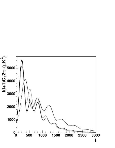
Figure 1: Three different CMB TT power spectra (up to $\ell_{\mathrm{max}}=3000$), used as illustrations for the method. The dark full line corresponds to WMAP data best fit model.

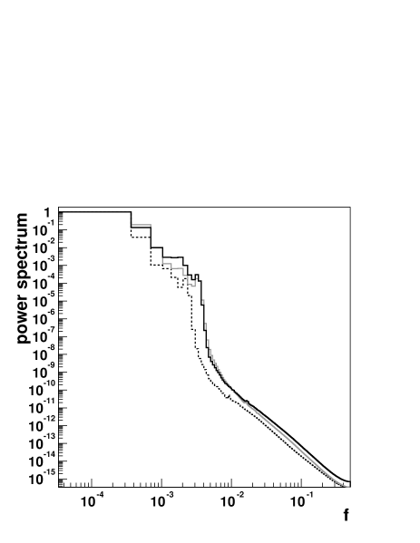
Figure 2: Power spectral densities (periodogram) of the three ${\cal{C}}_{\ell}$ spectra presented on Figure 1.

In each case, most of the power lies below $f_{\mathrm{max}}\simeq 0.005$ which corresponds to a minimum sampling rate of :

$$\Delta_{\text{min}}\simeq 100$$ (3)

This indicates that only 1 parameter on 100 ${{\cal{C}}_{\ell}}$ values is necessary to reconstruct the whole spectrum.

Fitting $\mn@boldsymbol{{{\cal{C}}_{\ell}}}$ spectra

When using the sampling rate $\Delta_{\ell}=\Delta_{\text{min}}$, some part of the Fourier spectrum is nonetheless removed, and the Shannon interpolation given by (2) is no longer exact. We therefore modify it to a linear parameterization :

$${\cal{C}}({l})=\sum_{j=1}^{N_{\mathrm{par}}}a_{j}u\left(\dfrac{l-l_{j}}{\Delta_{\ell}}\right)$$ (4)

where:

- the $\{a_{j}\}_{j=1,...,N_{\mathrm{par}}}$ represent a set of parameters to be estimated on the data through least square minimization.

- $u$ denotes the “basis” function and will be discussed more in details in the next part.

- the $\{l_{j}\}$ represent a grid of fixed points: $l_{j}=l_{0}+j\Delta_{\ell}$. Note that the first point ($l_{0}$) can be located anywhere. In practice one fixes it to the first measured multipole.

Eq. (4) denotes a decomposition of the ${\cal{C}}({l})$ function over the non-orthogonal basis $u_{j}(l)=u[(l-l_{j})/\Delta_{\ell}]$.

Given a set of “data” points, i.e. a set of ${\cal{C}}_{\ell}$ measurements and their covariance matrix, the parameters $\{a_{j}\}$ and their covariance matrix are determined through a simple linear least square fit. Then one has an estimate of the ${\cal{C}}({l})$ function for any real $\ell$ value together with its associated Gaussian error through standard error propagation (see section 3 for an example).

Bases

The sampling theorem uses the basis (denoted as Shannon):

$$u(x)=\operatorname{\sin_{\text{c}}}{(\pi x)}$$ (5)

It has the the nice property of being an exact interpolation on each point of the grid:

$$u(\dfrac{l_{i}-l_{j}}{\Delta_{\ell}})=\delta_{ij}$$ (6)

so that the estimated parameters ($\hat{a}_{j}$) satisfy:

$${\cal{C}}({l_{j}})=\hat{a}_{j}$$ (7)

and can be estimated “by eye” on a (perfect) ${\cal{C}}({l})$ curve.

However the Shannon basis is not strongly local in real space, involving long range correlations in the parameters covariance matrix.

To modify this behavior but still keeping the exact interpolation property, we multiply it by a Gaussian function and call this new basis Gauss-Shannon:

$$u(x)=\operatorname{\sin_{\text{c}}}{(\pi x)}\times\exp{(\dfrac{-x^{2}}{2\sigma^{2}})}$$ (8)

With respect to the Shannon basis, the off-diagonal terms of the parameters covariance matrix will be reduced. Although in principle one has the freedom to adjust the $\sigma$ of the Gaussian, it is more interesting to use “large” values, since in that case the bulk part of the Fourier spectrum is un-filtered : one just cuts off frequencies near $f_{\mathrm{max}}$ and the Shannon properties are (mostly) preserved. In the following we will therefore investigate the $\sigma=3$ case in Eq. (8).

For the sake of comparison, we will also investigate a very different basis provided by the simple Gaussian function (Gauss basis):

$$u(x)=\exp(\dfrac{-x^{2}}{2\sigma^{2}})$$ (9)

It does not have the exact interpolation property of Eq. (7) since it is always positive. Therefore the estimated parameters $\hat{a}_{j}$will now be very different from the ${\cal{C}}({l_{j}})$ function values, and the off-diagonal terms of the covariance matrix will be important. The Gaussian function is however the most rapidly decaying in both real and Fourier spaces (Hardy, 1933) and is therefore of great interest. If we want to perform a fit to Eq. (4), we do not have the freedom in the choice of $\sigma$. Indeed, since:

$$u(\frac{l}{\Delta_{\ell}})\xrightarrow{FT}\Delta_{\ell}U(\Delta_{\ell}f)\propto\exp(-2\pi^{2}(\Delta_{\ell}\sigma)^{2}f^{2})$$

by changing $\sigma$ we just define a new effective sampling rate. If we wish to keep the Shannon critical frequency of Eq. (1) we are lead to use $\sigma=1$ to avoid aliasing or over-sampling.

Edge effects

The Shannon theorem, on which is based the fit, is defined on an infinite support. By restricting the data to some measured $\ell$ range, a high frequency ringing appears near the boundaries. To reduce this phenomenon one can extend the grid beyond the data limits. Given the short range of the functions basis used in Eq.(4) , only one or two points can be added but this is sufficient in most of the cases. Note that we do not add any fake data, but just increase the grid position and number of parameters to be determined from the fit.

Results

To test the precision of the method, we fit the three ${\cal{C}}_{\ell}$ spectra of Figure 1. We use the Gauss-Shannon basis with a grid of 34 points ($\sl=100$ and 2 points added on the low-side $l<2$ and 1 on the high side $l>3000$). Since the input data has no error, their covariance matrix is defined as identity. Figure 3 shows the comparison of the parameterization and the genuine spectrum. A close-up of the low $\ell$ region is also displayed The agreement is very satisfactory up to very low $\ell$ values. The first few bins are not perfectly described because they introduce a high frequency component that is cutoff by the sampling rate of $\Delta_{\ell}=100$. This can be accounted for by a second step decomposition of the residuals as in a wavelet analysis. For the sake of simplicity and since experimental error bars are high in this region, we choose not to correct for this effect in the following. The upper part of the spectrum is correctly described.

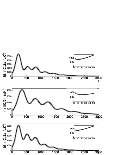
Figure 3: Superposition of the three input ${\cal{C}}_{\ell}$ spectra (dark thin line) from Figure 1, and the parameterizations described in the text (thick grey) . The Gauss-Shannon basis has been used, with a sampling rate of $\Delta_{\ell}=100$ and 2 extra-points on the low side and one on the high side (therefore 34 parameters have been fitted). The insets show a close-up of the low $\ell$ region. For the sake of visualization, the thick grey curves have been enlarged.

To compare the interest of using different bases, Figure 4 presents the relative agreement between the fitted values and the input WMAP best-fit model for the three bases: Shannon, Gauss-Shannon,Gauss. For the modified bases (Gauss-Shannon,Gauss) , the agreement is better than 1% in the range $\ell>30$. For low $\ell$ values the agreement decreases up to $\simeq 15\%$ for $\ell=2$.

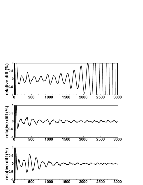
Figure 4: Relative agreement (in %) between the input ${\cal{C}}_{\ell}$ (WMAP best fit model) and the function obtained by fitting 34 parameters on the Shannon (upper plot), Gauss-Shannon (middle) and Gauss (bottom) bases

Both Gauss and Gauss-Shannon give very good results, Gauss being slightly more precise for the models we use. Recall however that the Gauss basis (unlike Gauss-Shannon) provides parameters with values far from the grid points and highly correlated. We will therefore prefer the Gauss-Shannon basis in the following.

Derived results

Once the parameters $\hat{a}_{j}$have been determined, including their covariance matrix $\hat{\mn@boldsymbol{V_{a}}}$, one can derive easily many characteristics of the spectrum.

${\cal{C}}_{\ell}$ values can be estimated for any (real) $l$ value. Using again the notation $u_{j}(l)=u[(l-l_{j})/\Delta_{\ell}]$:

$$\begin{split}\hat{{{\cal{C}}_{\ell}}}&=\sum_{j=1}^{N_{\mathrm{par}}}\hat{a}_{j}u_{j}(l)\\ \hat{\sigma}_{l}^{2}&=\mn@boldsymbol{U}\hat{\mn@boldsymbol{V_{a}}}\mn@boldsymbol{U}^{T}\end{split}$$ (10)

$\mn@boldsymbol{U}$ being the vector of components $U_{j}=u_{j}(l)$.

The peak (and dip) locations can be determined by setting the derivatives of Eq. (4) to zero and finding (numerically) the roots.

One can compute also binned values. For a given binning $(b_{1},b_{2},..,b_{N})$, assuming a weighting scheme $w_{i}^{b}$ inside the bin $b$:

$$\hat{{{\cal{C}}_{\ell}}}^{b}=1/W_{b}\sum_{l\in b}w_{i}^{b}\hat{{{\cal{C}}_{\ell}}}$$ (11)

with the normalization $W_{b}=\sum_{l\in b}w_{i}^{b}$.

The covariance matrix of the binned estimate is obtained again through error propagation $\mn@boldsymbol{B}=\mn@boldsymbol{D}\hat{\mn@boldsymbol{V_{a}}}\mn@boldsymbol{D}^{T}$, $\mn@boldsymbol{D}$ being a ($N\times N_{\mathrm{par}}$) matrix defined by:

$$D_{bj}=1/W_{b}\sum_{l\in b}w_{i}^{b}u_{j}(l)$$ (12)

3 Application to WMAP data

We now turn on to real data, by describing the WMAP TT angular power spectrum .

The data consist of a sample of N=899 measurements for integer $\ell$ values in the [2,900] range, and of the weight matrix (inverse covariance) $\mn@boldsymbol{W}$ defined as the Fisher matrix for the ML estimate.

We begin with a check of our ${\cal{C}}_{\ell}$ smoothness hypothesis, showing the periodogram of the data on Figure 5. Unlike Figure 2, this one has (statistical) noise, described by the covariance matrix of the data ($\mn@boldsymbol{C}$). We estimate the mean level of noise power in each Fourier mode $k$ by:

$$<\lvert n_{k}\rvert^{2}>=\sum_{l=0}^{N-1}\sum_{m=0}^{N-1}\exp[j\dfrac{2\pi}{N}(l-m)k]\mn@boldsymbol{C}_{lm}$$ (13)

and show it on the Figure too.

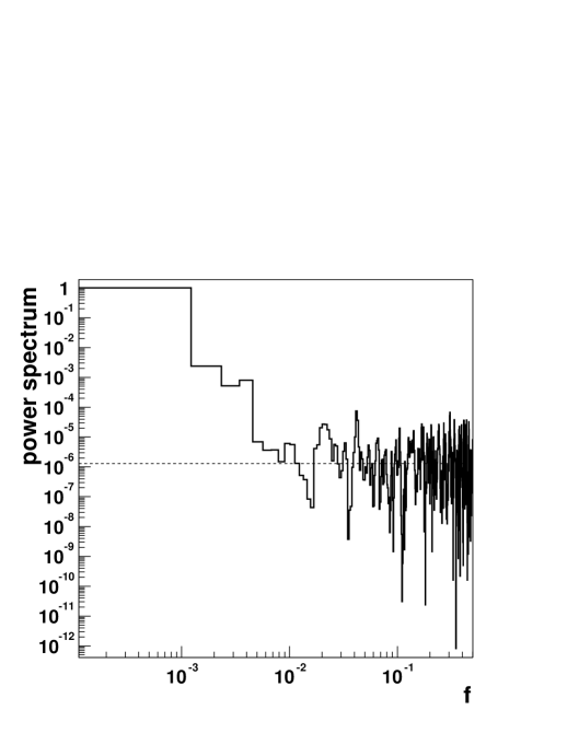
Figure 5: Power spectrum estimated through the periodogram of WMAP data. The dashed line corresponds to the estimate of the mean level of noise.

The (noise subtracted) signal does not show high frequency components and we keep the cut $f_{\mathrm{max}}=0.005$ determined previously, leading to the sampling rate $\Delta_{\ell}=100$. We then choose the Gauss-Shannon basis and put 10 $l_{j}$ knots between 2 and 900. We add two extra-points on the low $\ell$ side and one on the high side. We are therefore left with determining 13 parameters from a set of N=899 input data.

The (linear) least square estimate reads:

$$\begin{split}\hat{\mn@boldsymbol{a}}&=(\mn@boldsymbol{AWA})^{-1}\mn@boldsymbol{A^{T}W}\mn@boldsymbol{c}\\ \hat{\mn@boldsymbol{V_{a}}}&=(\mn@boldsymbol{AWA})^{-1}\end{split}$$ (14)

with

$$\mn@boldsymbol{A}_{ij}=u(\dfrac{\ell_{i}-\ell_{j}}{\Delta_{\ell}})$$ (15)

and $\mn@boldsymbol{c}$ is the input data values vector.

There is a subtlety however. The Fisher matrix (or “curvature” as defined in Verde et al. (2003)) depends actually on the true ${\cal{C}}_{\ell}$ distribution through the cosmic variance. We need a means to incorporate it in our fits, in particular for the low $\ell$ range. This is performed through the following iterative procedure: we start from the WMAP best ${\cal{C}}_{\ell}$ estimates (as true values) to obtain the weight matrix, and perform the fit. We then recompute the weight from the Fisher matrix using this time the fitted ${\cal{C}}_{\ell}$ values, and redo the fit. We pursue the iteration until the $\chi^{2}$ gets stable.

For this data set, the fit is stable after 3 iterations.

Figure 6 shows the result of the last fit.

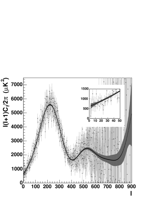
Figure 6: Result of the parameterization performed on WMAP data using the Gauss-Shannon basis. Light grey points corresponds to WMAP data for each integer $\ell$. Their error is computed from the diagonal elements of the inverse of the Fisher matrix as obtained in the last step of the iterative procedure described in the text. The dark line corresponds to our best estimate for each integer $\ell$ and the errors (dark grey area) are computed from the parameters covariance matrix through standard error propagation. A close-up of the low $\ell$ region is also shown.

The $\chi^{2}$ per degree of freedom is excellent: $959/886$. Figure 7 shows the “pull” distribution that we define as the data value minus the estimated value divided by the data error. Here again the data errors are obtained from the diagonal elements of the inverse of the Fisher matrix. The distribution is compatible with a normal one. We checked that this feature is valid over the whole $\ell$ range. These results indicate that the data are consistent with the assumption of a smooth power spectrum.

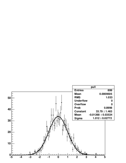
Figure 7: “Pull” distribution of WMAP data w.r.t to our best fit estimate. Also superimposed is the fit to a gaussian function. The parameters of the histogram and the result of the fit are given in the box.

As is clear from Figure 6 our fitted function (which includes the effect of the cosmic variance) has a positive slope in the low $\ell$ region.

Finally we provide the parameterization obtained in Table 1 (parameters) and Figure 8 (correlation matrix). It represents the most probable estimate of the band limited ${\cal{C}}_{\ell}$ spectrum and one can derive several secondary results as explained in section 2. Note how the parameter values can be determined directly from Figure 6, as expected for the Gauss-Shannon basis. The off-diagonal terms of the parameters matrix have also been reduced w.r.t a simple Shannon based fit.

The three bases give however similar results for the final fitted function.

We emphasize once more that this description is independent from any cosmological model.

parameter index $j$	grid position $l_{j}$	estimated parameters $\hat{a}_{j}$
0	$-197.6$	$15.1\pm 16087.1$
1	$-97.8$	$-415.9\pm 8077.1$
2	$2.0$	$639.9\pm 129.8$
3	$101.8$	$2679.8\pm 36.4$
4	$201.6$	$5472.4\pm 58.6$
5	$301.3$	$3892.7\pm 43.6$
6	$401.1$	$1649.7\pm 37.4$
7	$500.9$	$2379.8\pm 66.6$
8	$600.7$	$2098.0\pm 124.6$
9	$700.4$	$1683.9\pm 252.8$
10	$800.2$	$1831.2\pm 559.8$
11	$900.0$	$4953.8\pm 2384.6$
12	$999.8$	$6123.9\pm 7475.2$

Table 1: Value of the parameters (and grid spacing) obtained from the fit to WMAP data on the Gauss-Shannon basis.

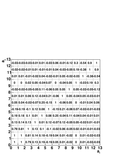
Figure 8: Correlation matrix of the parameters determined from the fit of WMAP data on the Gauss-Shannon basis.

4 Other power spectra

4.1 Fourier transform of rings $\Gamma_{m}(\theta)$

For a circular scanning strategy, the Fourier decomposition of circles is an interesting analysis method , since it does not use map projection and allows to follow in time the detector response, avoiding hypotheses such as noise stationarity.

The power spectrum is simply related to the underlying $C_{\ell}$ through (Delabrouille et al., 1998)

$${\Gamma_{m}(\theta)}=\sum_{\ell\geq m}{\cal P}_{l}^{m}(\cos\theta)^{2}B_{l}^{2}C_{\ell}$$ (16)

where

1. $\theta$ is the opening angle on the sky (colatitude)

2. ${\cal P}_{l}^{m}$ denote the (normalized) associated Legendre polynomials

3. $B_{l}$ is the beam transfer function, depending just on $\ell$ for a Gaussian symmetric beam.

The inverse process of retrieving $C_{\ell}$ values from a set of measured $\Gamma_{m}(\theta)$ is delicate due to the fact that ${\cal P}_{l}^{m}(\cos\theta)\rightarrow 0$ when $\ell>m/\sin\theta$. Ansari et al. (2003) have shown formally how a Fourier scaling in the flat sky limit allows to invert the problem up to very low $\ell$ values ($\ell\ga 3$ for ($\theta=40^{\circ}$)). The key point in their approach is to interpolate the $\Gamma_{m}(\theta)$ spectrum to non-integer $m$ values ($m/\sin\theta$) which can be done with the present method, since the $m{\Gamma_{m}(\theta)}$ spectrum is smooth. It is simpler however to stay in the $\ell$ space and use the previous results.

We describe again the ${\cal{C}}({l})$ function in terms of eq. (4). By combining with Eq. (16) :

$${\Gamma_{m}(\theta)}=\sum_{j}a_{j}\left[\sum_{\ell\geq m}\dfrac{2\pi B_{\ell}^{2}}{\ell(\ell+1)}{\cal P}_{l}^{m}(\cos\theta)^{2}u(\dfrac{\ell-l_{j}}{\Delta_{\ell}})\right]$$ (17)

which is still linear in the $a_{j}$.

The $a_{j}$ parameters can therefore be fitted directly on the $\Gamma_{m}(\theta)$  data using the above new basis, and the ${\cal{C}}_{\ell}$ spectrum is still obtained from Eq.(4).

Note that this approach allows to combine any number of detectors with different opening angles and transfer functions.

4.2 Angular power spectrum $C(\theta)$

Using again the decomposition (Eq. (4)) , the two-point angular correlation function can be expressed linearly in terms of the $a_{j}$:

$${C(\theta)}=\sum_{j}a_{j}\left[\sum_{\ell}\dfrac{2\ell+1}{2\ell(\ell+1)}P_{l}(\cos\theta)u(\dfrac{\ell-l_{j}}{\Delta_{\ell}})\right]$$ (18)

The same approach than in the previous part is therefore possible. Although equivalent to the usual methods, it allows to drop the $a_{lm}$ computations and adjust directly the ${\cal{C}}_{\ell}$ distribution, even on partial or masked sky data.

5 Conclusion

In this article, we take advantage of the smoothness of the ${\cal{C}}_{\ell}$ power spectra to decompose the signal in Fourier space and apply an improved version of the sampling theorem. We obtain an accurate parameterization of the spectra, that is independent from cosmological models, as a function ${\cal{C}}({l})$ for real $l$, with few parameters: for “reasonable” CMB models we find that sampling the ${\cal{C}}_{\ell}$ spectrum with one point on 100 is sufficient to retrieve the signal on any $\ell$ range at the percent level, down to very low $\ell$ values. We also show how this kind of description can be applied to other CMB power spectra as the Fourier spectrum of rings ($\Gamma_{m}(\theta)$) or the angular correlation function ($C(\theta)$).

We apply the method to WMAP first year data and provide the complete parameterization of the ${\cal{C}}_{\ell}$ spectrum. We show that the data is consistent with the expected smoothness of the spectrum.

Such a parameterization is richer than peaks determination (which can obviously be derived from it). It also allows the combination of various experiments and a $\chi^{2}$ test of the compatibility between them based on the assumed smoothness of the spectrum.

Finally it can allow to compress the data (by a factor $\simeq 100$) for the storage of cosmological models used in large databases.

The method can be applied to any band-limited function to be adjusted on data.

References

- (1)
- Ansari et al. (2003) R. Ansari, S. Bargot, A. Bourrachot, F. Couchot, J. Haïssinski, S. Henrot-Versillé, G. Le Meur, O. Perdereau, M. Piat, S. Plaszczynski, F. Touze, 2003, MNRAS, 343, 552
- Bennet et al. (2003) C. L Bennet et al., 2003, ApJS, 148, 1
- Bartlett (1999) Bartlett J., 1999, New Astron.Rev. 43, 83
- Delabrouille et al. (1998) Delabrouille, J., Gorski, K. M., Hivon E., 1998, MNRAS, 298, 445
- Douspis and Ferreira (2002) Douspis M., Ferreira P., 2002, Phys. Rev. D, 65, 087302
- Durrer et al. (2003) Durrer, R., Novosyadlyj, B., Apunevych, S., 2003, ApJS, 583, 33
- Hardy (1933) Hardy G.H, 1933, Journal of the London Mathematical Society, vol. 8, pp. 227-231
- Hinshaw et al. (2003) G. Hinshaw et al., 2003, ApJS, 148, 135
- Hu et al. (2001) Hu W., Fukugita M., Zaldarriaga M., Tegmark M., 2001, ApJ, 549, 669
- Hu and Dodelson (2002) Hu W., Dodelson S., 2002, ARA&A, 40, 171
- Knox and Page (2000) Knox L. and Page L., 2000, Phys. Rev. Lett. 85, 1366
- Ödman et al. (2003) Ödman C. J., Melchiorri A., Hobson M. P., Lasenby A. N., 2003, Phys. Rev. D, 67, 083511
- Ödman (2003) Ödman C. J., astro-ph/0305254
- Oh et al. (1999) Oh S.P., Spergel D., Hinshaw G., 1999, ApJ, 510, 551
- Spergel et al. (2003) D. N Spergel et al., 2003, ApJS, 148, 175
- Verde et al. (2003) L. Verde et al., 2003, ApJS, 148, 195