Diffuse X-rays from the Inner 3 Parsecs of the Galaxy

Abstract

Recent observations with the Chandra X-ray Observatory have provided us with the capability to discriminate point sources, such as the supermassive black hole Sgr A*, from the diffuse emission within the inner $10^{\prime\prime}$ of the Galaxy. The hot plasma producing the diffuse X-radiation, estimated at $\approx 7.6\times 10^{31}$ ergs s^-1 arcsec^-2 in the 2–10 keV band, has a RMS electron density $\approx 26$ cm^-3 and a temperature $kT\approx 1.3$ keV, with a total inferred mass of $\approx 0.1\;M_{\odot}$. At least some of this gas must be injected into the ISM via stellar winds. In the most recent census, about 25 bright, young stars have been identified as the dominant sources of the overall mass efflux from the Galactic center. In this paper, we use detailed 3-dimensional SPH simulations to study the wind-wind interactions occurring in the inner 3 parsecs of the Galaxy, with a goal of understanding what fraction, if any, of the diffuse X-ray flux measured by Chandra results from the ensuing shock heating of the ambient medium. We conclude that this process alone can account for the entire X-ray flux observed by Chandra in the inner $10^{\prime\prime}$ of the Galaxy. Understanding the X-ray morphology of the environment surrounding Sgr A* will ultimately provide us with a greater precision in modeling the accretion of gas onto this object, which appears to be relatively underluminous compared to its brethren in the nuclei of other galaxies.

1 Introduction

The inner few parsecs of the Galaxy contain several observed components that coexist within the central deep gravitational potential well. The pointlike, nonthermal radio source Sgr A* appears to be the radiative manifestation of a $\sim 3$ million M_⊙ concentration of dark matter within $\sim 0.015$ pc of the nucleus. This concentration, probably a central black hole, is surrounded by a cluster of evolved and young stars, a molecular dusty ring, ionized gas streamers, diffuse hot gas and Sgr A East, a shell-like, nonthermal radio source believed to be the remnant (SNR) of a supernova explosion at the center of the Galaxy some $10,000$ years ago (see Melia & Falcke, 2001).

Observations at infrared and, particularly, radio wavelengths have been very effective in unraveling the complex behavior of the central components through their mutual interactions. But only through recent observations with the Chandra X-ray Observatory have we been able to study the X-ray emission from Sgr A* and its surroundings with sub-arcsecond resolution and a broad X-ray band imaging detector. These capabilities have provided us with the means to discriminate point sources, such as Sgr A*, from the diffuse emission due to hot plasma in the ambient medium.

Baganoff et al. (2003) report that the Chandra/ACIS-I 0.5–7 keV image of the inner $17^{\prime}\times 17^{\prime}$ region of the galaxy contains remarkable structure; its detail is sufficient to allow comparisons with features seen in the radio and IR wavebands. The diffuse X-ray emission is strongest in the center of Sgr A East. Based on these X-ray observations, Maeda et al. (2001) conclude that Sgr A East is a rare type of metal-rich, “mixed-morphology” SNR that was produced by the Type II explosion of a 13–20 $M_{\odot}$ progenitor. The X-ray emission from Sgr A East appears to be concentrated within the central 2–3 pc of the $6\times 9$ pc radio shell and is offset by about $2$ pc from Sgr A* itself. The thermal plasma at the center of Sgr A East has a temperature $kT\approx 2$ keV, and appears to have strongly enhanced metal abundances with elemental stratification.

However, this is not the sole component of hot gas surrounding Sgr A*. Chandra has also detected X-ray emission extending perpendicular to the Galactic plane in both directions through the position of Sgr A*, which would seem to indicate the presence of a hot, “bipolar” outflow from the nucleus. And an additional component of X-ray emitting gas appears to have been found within the molecular ring, much closer to Sgr A*. Indeed, the western boundary of the brightest diffuse X-ray emission within $2$ pc of the Galactic center coincides very tightly with the shape of the Western Arc of the thermal radio source Sgr A West. Given that the Western Arc is believed to be the ionized inner edge of the molecular ring, this coincident morphology suggests that the brightest X-ray emitting plasma is being confined by the western side of the gaseous torus. In contrast, the emission continues rather smoothly into the heart of Sgr A East toward the eastern side.

A detailed fit of the emission from the hot gas within $10^{\prime\prime}$ of Sgr A* shows that it is clearly not an extension of the X-ray emitting plasma at the center of Sgr A East. The inferred 2–10 keV flux and luminosity of the local diffuse emission are $(1.9\pm 0.1)\times 10^{-15}$ ergs cm^-2 s^-1 arcsec^-2 and $(7.6^{+2.6}_{-1.9})\times 10^{31}$ ergs s^-1 arcsec^-2, respectively. Based on the parameters of the best-fit model, it is estimated that the local, hot diffuse plasma has a RMS electron density $\langle n_{e}^{2}\rangle^{1/2}\approx 26$ cm^-3. Assuming that this plasma has a filling factor of unity and is fully ionized with twice solar abundances, its total inferred mass is $M_{\hbox{\rm local}}\approx 0.1\;M_{\odot}$. The local plasma around Sgr A* appears to be distinctly cooler than the Sgr A East gas, with a temperature $kT=1.3^{+0.2}_{-0.1}$ keV. By comparison, the best-fit model for Sgr A East indicates that the plasma there has about 4 times solar abundances, and twice this temperature (see above).

At least some of this local, hot plasma must be injected into the ISM via stellar winds. There is ample observational evidence in this region for the existence of rather strong outflows in and around the nucleus. Measurements of high velocities associated with IR sources in Sgr A West (Krabbe et al., 1991) and in IRS 16 (Geballe et al., 1991), the $H_{2}$ emission in the molecular ring and from molecular gas being shocked by a nuclear mass outflow (Gatley et al., 1986; but see Jackson et al., 1993 for the potential importance of UV photodissociation in promoting this $H_{2}$ emission), broad Br$\alpha$, Br$\gamma$ and He I emission lines from the vicinity of IRS 16 (Hall, Kleinmann & Scoville, 1982; Allen, Hyland & Hillier, 1990; Geballe et al., 1991), and radio continuum observations of IRS 7 (Yusef-Zadeh & Melia, 1991), provide clear evidence of a hypersonic wind, with a velocity $v_{w}\sim$ 500–1,000 km s^-1, a number density $n_{w}\sim 10^{3\mbox{--}4}$ cm^-3, and a total mass loss rate $\dot{M}_{w}\sim$ 3–4 $\times 10^{-3}\;M_{\odot}$ yr^-1, pervading the inner parsec of the Galaxy.

Chevalier (1992) discussed the properties of stellar winds in the Galactic center and their ability to produce X-rays, under the assumption that the colliding winds create a uniform medium with a correspondingly uniform mass and power input within the central 0.8 pc of the Galaxy. While the assumption of uniformity may be an over-simplification, steady-state models yield central conditions similar to those calculated in our simulations and (apparently) observed in nature.

The possibility that wind-wind collisions in the dense stellar core of the Galaxy might produce an observable X-ray signature was considered more recently in the context of transient phenomena by Ozernoy et al. (1997). These authors argued that the strong winds from OB stars or WR stars would produce shocks that heat the gas up to a temperature $T\sim 10^{7}$ K. Instabilities in the overall outflow could therefore produce transient high temperature regions, in which the X-ray luminosity could be as high as $10^{33}$–$10^{35}$ ergs s^-1.

A preliminary, low-resolution 3-dimensional hydrodynamical simulation by Melia & Coker (1999) subsequently revealed that although the tesselated pattern of wind-wind collision shocks can shift on a local dynamical time scale, the overall concentration of shocks in the central region remains rather steady. This is hardly surprising, given that 25 or so dominant wind sources are distributed rather evenly about the center.

In this paper, we study in detail the emission characteristics of shocked gas produced in wind-wind collisions within 3 parsecs of Sgr A*. We present the results of comprehensive, high-resolution numerical simulations of the wind-wind interactions, using the latest suite of stellar wind sources with their currently inferred wind velocities and outflow rates. We use their projected positions and vary the radial coordinates to determine the effect of this uncertainty on the X-ray emissivity. In addition, it is clear now from the Chandra image that the stellar winds are also interacting directly with the molecular ring, and so we incorporate the latter into the set of boundary conditions for our simulations. The predicted X-ray luminosity and spatial profile may then be compared with the Chandra data. We describe our numerical technique, including the description of this molecular ring and the characteristics of the wind sources in § 2 of the paper. In § 3 we present our results, and discuss their implications for the conditions in the Galactic center in § 4.

2 The Physical Setup

Our calculations use the 3-dimensional smoothed particle hydrodynamics (SPH) code discussed in Fryer & Warren (2002), and Warren et al. (2003). The Lagrangean nature of SPH allows us to concentrate spatial resolution near shocks and capture the complex time-dependent structure of the shocks in the Galactic center.

We assume that the gas behaves as an ideal gas, using a gamma-law ($\gamma=5/3$) equation of state. Since the mass of gas in the simulation at any time is many orders of magnitude less than the mass of the black hole and its halo of stars, we calculate gravitational effects using only the gravitational potential of the assumed central $2.6\times 10^{6}\;M_{\odot}$ point mass.

Each of our two calculations uses slightly different initial conditions; details of each calculation are summarized in Table 1. The initial conditions for each simulation assume that the Galactic center has been cleared of all mass (perhaps by the supernova explosion that produced Sgr A East). Massive stars then inject mass into the volume of solution via winds, gradually increasing the mass of gas in the Galactic center. The number of particles in each simulation initially grows rapidly, but reaches a steady state ($\sim 7$ million particles) when the addition of particles from wind sources is compensated by the particle loss as particles flow out of the computational domain or onto the central black hole. The particle masses vary from $9.4\times 10^{-7}\;M_{\odot}$ to $1.0\times 10^{-5}\;M_{\odot}$.

In addition, we place a torus of molecular material in a circumnuclear disk surrounding the inner 1.2 pc of the Galaxy. The boundary conditions (outer and central black hole), the circumnuclear disk, and the stellar wind sources are the only modifications made to the basic SPH code of Warren et al. (2003) to run these simulations, and we discuss these modifications in more detail in the next three subsections.

2.1 Boundary Conditions

The boundary conditions are the major particle sinks in the simulation. We assume that once these particles have achieved escape velocity beyond a certain distance, nothing confines the material flowing out of the Galactic center. The computational domain is a cube approximately $6$ pc on a side, centered on the black hole. To simulate “flow-out” conditions, particles passing through this outer boundary are removed from the calculation.

In addition, particles passing through an inner spherical boundary with a radius of $1.9\times 10^{17}$ cm (equivalent to $2.5\times 10^{5}$ R_s or $\sim 0.7$ Bondi-Hoyle capture radii for Sgr A*) centered on the black hole are also removed. This assumes that the accretion onto Sgr A* continues roughly at free-fall below this point. Such a simplified assumption only provides a limit on the X-ray luminosity of the point-source of Sgr A*, but it does not affect the diffuse X-ray emission in the Galactic center that is the central topic of this paper.

2.2 Circumnuclear Disk

HCN synthesis data, taken at $5^{\prime\prime}-10^{\prime\prime}$ spatial and $4$ km s^-1 spectral resolution, reveal a highly inclined, clumpy ring of molecular gas surrounding the ionized central $\sim 2$ pc of the Galaxy (Güsten et al., 1987). This ring seems to be the inner edge of a thin molecular structure extending out to $\sim 5-7$ pc from the center. Within this cavity, and orbiting about Sgr A*, is the huge H II region known as Sgr A West comprised of a 3-armed mini-spiral (Lo & Claussen, 1983; Lacy et al., 1991). The molecular and ionized gas in the central cavity appear to be coupled, at least along the so-called western arc (one of the spiral arms), which appears to be the ionized inner surface of the molecular ring. It has been suggested that the northern and eastern arms may be streamers of ionized gas falling toward Sgr A* from other portions of the molecular ring (see Melia & Falcke, 2001, and references cited therein).

Since 1987, observations of various tracers of molecular gas (notably H₂, CO, CS, O I, HCN, NH₃) have somewhat refined our view of the circumnuclear disk (or CND, as it is sometimes called), leaving us with the following set of defining characteristics: a total mass of $\sim 3\times 10^{4}\;M_{\odot}$, a very clumpy distribution with an estimated volume filling factor of $\sim 0.01$, a typical clump mass of $\sim 30\;M_{\odot}$, size $\sim 0.1$ pc, and temperature $\sim 100$ K (see Gatley et al., 1986; Serabyn et al., 1986; Güsten et al., 1987; DePoy et al., 1989; Sutton et al., 1990; Jackson et al., 1993; Marr et al., 1993). As many as $500$ clumps fill its overall structure. Its height at the inner edge is $\sim 0.5$ pc, and it flares outward with distance from the center.

The Chandra $0.5-7$ keV image of the central $1.3^{\prime}\times 1.5^{\prime}$ region of the Galaxy (see Fig. 4 in Baganoff et al., 2003), overlaid on the VLA 6-cm contours of Sgr A* and Sgr A West, shows that the western boundary of the brightest diffuse X-ray emission coincides very closely with the shape of the western arc, adding credence to the notion that the latter tracks the inner edge of the CND if one adopts the view that the X-ray glowing plasma is itself being confined by the western side of the molecular ring.

The CND therefore appears to be an essential element in the (partial) confinement of the hot gas, and we incorporate it into our simulations using a simple approach that nonetheless retains the CND’s important features. To keep the volume of solution tractable, we do not model the entire $\sim 14$-pc disk, but rather introduce an azimuthally-symmetric torus with inner radius $1.2$ pc (see Güsten et al., 1987) and thickness $1$ pc. The latter is a fair representation of the CND’s observed height at this radius. This structure does not, of course, account for the CND’s outer regions, but as we shall see, the hot, X-ray emitting gas does not penetrate far into the molecular boundary, so the outer CND is not directly relevant to this simulation. We assume that this torus has a mass of $\sim 10^{4}\;M_{\odot}$, and is composed of 200 spherical clumps, each of mass $50\;M_{\odot}$. We also incline it by $60^{\circ}$ from the plane of the sky, orienting its principal axis (in projection) along the Galactic plane.

2.3 Wind Sources

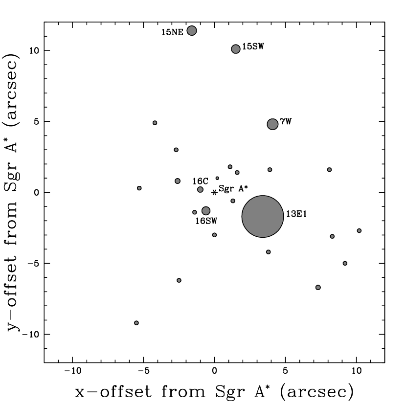
Figure 1: Location of the 25 wind-producing stars used in the simulations reported here, relative to the position of Sgr A* indicated by the * symbol. The radius of each circle corresponds (on a linear scale) to that star’s mass loss rate. Setting the scale is 13E1, with $\dot{M}=7.9\times 10^{-4}\;M_{\odot}$ yr^-1.

It is well known by now that the Galactic center wind is unlikely to be uniform, since many stars contribute to the mass ejection (see, e.g., Melia & Coker, 1999). For these calculations, we assume that the early-type stars enclosed (in projection) within the Western Arc, the Northern Arm, and the Bar produce the observed wind. Thus far, 25 such stars have been identified (Genzel et al., 1996), though the stellar wind characteristics of only 8 have been determined from their He I line emission (Najarro et al., 1997). Figure 1 shows the positions (relative to Sgr A*; $1^{\prime\prime}\approx 0.04$ pc at the Galactic center) of these wind sources; the size of the circle marking each position corresponds to the relative mass loss rate (on a linear scale) for that star. IRS 13E1 and IRS 7W seem to dominate the mass outflow with their high wind velocity ($\sim$ 1,000 km s^-1) and a mass loss rate of more than $2\times 10^{-4}\;M_{\odot}$ yr^-1 each.

Wind sources are modeled as literal sources of SPH particles. New particles are added in shells around each wind source as the simulation progresses and the existing particles move outward from each source. Using wind velocities inferred from observations (Najarro et al., 1997), shells around each wind source are added at a rate such that the spacing between shells is approximately equal to the spacing between particles within each incoming shell. Masses of the incoming particles are chosen to match the inferred mass loss rate for each source. The stars without any observed He I line emission are assigned a wind velocity of 750 km s^-1 and an equal mass loss rate chosen such that the total mass ejected by the stars used here is equal to $3\times 10^{-3}\;M_{\odot}$ yr^-1, the overall mass outflow inferred for the Galactic center region (see, e.g. Melia, 1994). The initial temperature of the stellar winds is not well known; for simplicity, we assume here that all the winds are Mach 30 at their point of ejection from the stellar surface. This corresponds to a gas temperature of $\sim 10^{4}$ K. We note, however, that our results are insensitive to this value, since the temperature of the shocked gas is set primarily by the kinetic energy flux carried into the collision by the winds. For the calculations reported here, the sources are assumed to be stationary over the duration of the simulation.

An additional uncertainty is the location in $z$ (i.e., along the line of sight) of the wind sources. To test the sensitivity of our results to the choice of $z$, we carry out two simulations with different coordinate assignments, and compare the overall shocked gas configurations and their X-ray emissivities. For the first choice of $z$ positions—listed as $\rm z_{1}$ in Table 2 and used in Simulation 1—we determine this third spatial coordinate randomly, subject to the condition that the overall distribution in this direction matches that in $x$ and $y$. With this proviso, all these early-type stars are located within the central few parsecs surrounding Sgr A*. For the second choice of positions—listed as $\rm z_{2}$ and used in Simulation 2—we attempt to calculate a reasonable upper limit on the luminosity produced in the central parsec by moving all the sources closer together in $z$, toward the $z=0$ plane.

3 The Gas Profile and Spectrum

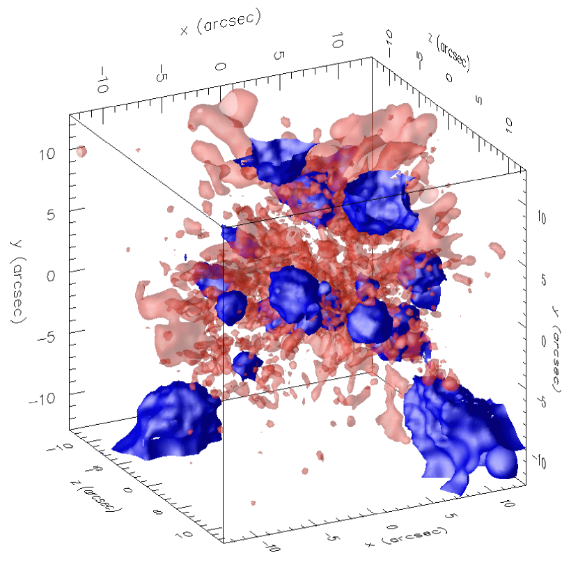
Figure 2: Isosurfaces of specific internal energy from Simulation 1, $10,000$ years after the winds were turned on. The blue surfaces correspond to a specific internal energy of $2.5\times 10^{12}$ ergs g^-1; the red surfaces correspond to $3.8\times 10^{15}$ ergs g^-1.

Wind-wind collisions in the central parsec create a complex configuration of shocks that efficiently converts the kinetic energy of the winds into internal energy of the gas. Figure 2 shows isosurfaces of specific internal energy in the central cubic parsec of Simulation 1, $\sim~{}10,000$ years after the beginning of the calculation. The blue surfaces indicate regions of gas with low specific internal energy, which lie near the wind sources; the red surfaces mark regions of high specific internal energy, where gas has passed through multiple shocks. 26% of the total energy in the central parsec has been converted to internal energy via multiple shocks: the total kinetic energy of material in the central parsec is $7.7\times 10^{48}$ ergs, while the total internal energy is $2.7\times 10^{48}$ ergs.

In order to calculate the observed continuum spectrum, we assume that the observer is positioned along the negative $z$-axis at infinity and we sum the emission from all of the winds—and their shocks—produced by the 25 stars in Table 2. For the conditions we encounter here, scattering is negligible and the optical depth is always less than unity. For these temperatures and densities, the dominant components of the continuum emissivity are electron-ion ($\epsilon_{ei}$) and electron-electron ($\epsilon_{ee}$) bremsstrahlung.

Figures 3 and 4 show the 2–10 keV luminosity per arcsec² from the central 10^′′ of Simulations 1 and 2, respectively, versus time since the beginning of each calculation. The winds fill the volume of solution after $\sim$ 4000 years, which coincides with the point in each figure where the luminosity stops rising rapidly and begins varying by only $\sim$ 5% around a steady value. The inset plot in each figure shows variation of the luminosity on a timescale of $\sim$ 10 years. Data points in the insets are plotted for each of 990 time steps, where the size of each time step is 0.16 years. Variation between consecutive data points is due primarily to numerical noise, but variations on timescales of several years indicate noticeable changes in the temperature and density of the gas in the central 10^′′.

The range of values of the average luminosity per arcsec² measured in the central 10^′′ of our simulations illustrates the sensitivity of the luminosity to the positions of the wind sources. Luminosities for each of our simulations are reported in Table 1; for comparison, Baganoff et al. reported a 2–10 keV luminosity of $(7.6^{+2.6}_{-1.9})\times 10^{31}$ ergs s^-1 arcsec^-2 from the local diffuse emission within 10^′′ of Sgr A*. Results from both simulations fall within the error bars reported by Baganoff et al.

Table 1 also includes two different estimates for the temperature of the plasma within 10^′′ of Sgr A*. T_mass is an average temperature calculated using the mass of each particle as a weighting factor, while T_lum uses the luminosity of each particle as a weighting factor. Since the temperature is determined primarily by the kinetic energy flux initially carried by the winds, and since the initial wind velocities in each calculation are the same, the average temperature for the plasma at the center of each calculation is essentially the same.

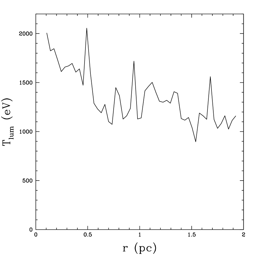
Figure 6: Average luminosity-weighted temperature per 0.035 pc radial “bin” versus distance from the central black hole in Simulation 1. Collisions between the winds and the inner edge of the CND are visible as a spike near 1 pc.

Figures 5 and 6 show the average luminosity per volume and average luminosity-weighted temperature as a function of radius from the center of Simulation 1. The majority ($77\%$ of the overall 2–10 keV luminosity) of the 2–10 keV emission comes from the central 0.4 pc, where it is produced in wind-wind collisions. There is also noticeable emission ($2.5\%$ of the overall luminosity) from a high-temperature region centered on 1.2 pc, which is the location of the inner edge of the CND; emission here is produced when winds collide with the clumps in our model torus.

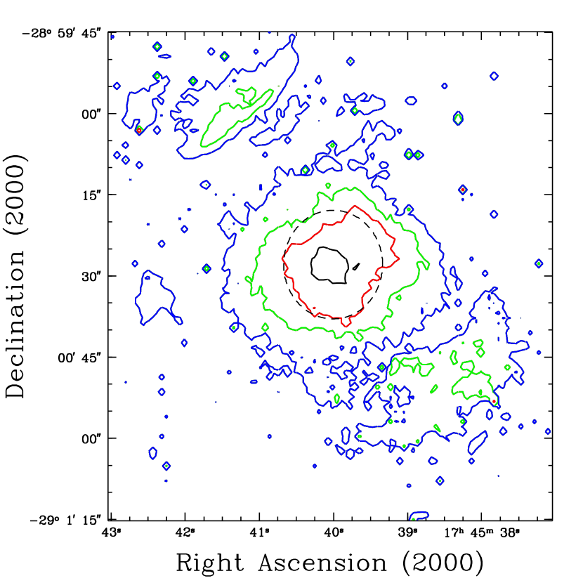
Figure 7: Contours of column-integrated 2–10 keV X-ray luminosity per “bin” from Simulation 1. There are 100 bins along each axis; each bin is 0.9^′′ by 0.9^′′. In order from black to red to green to blue, the luminosities indicated by the contours are $10^{32}$ ergs s^-1 per bin, $10^{31}$ ergs s^-1 per bin, $10^{30}$ ergs s^-1 per bin, and $1.5\times 10^{29}$ ergs s^-1 per bin. The dashed circle indicates the extent of the “local” region around Sgr A*; it has a radius of $10^{\prime\prime}$ and is centered on Sgr A*.

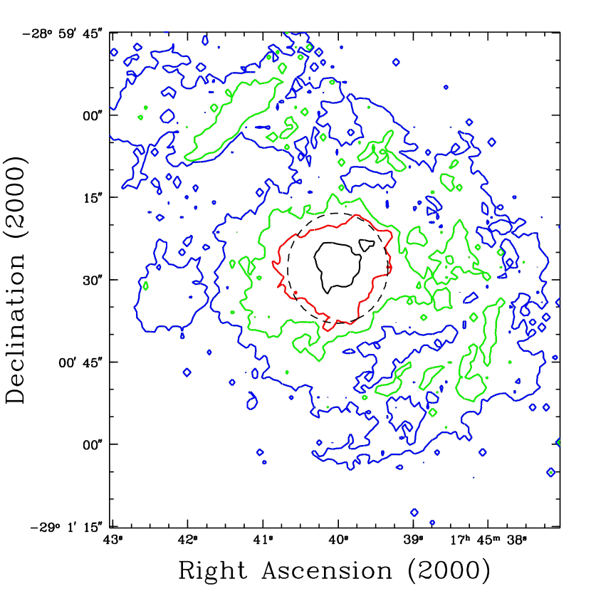
Figure 8: Contours of column-integrated 2–10 keV X-ray luminosity per “bin” from Simulation 2. There are 100 bins along each axis; each bin is 0.9^′′ by 0.9^′′. In order from black to red to green to blue, the luminosities indicated by the contours are $10^{32}$ ergs s^-1 per bin, $10^{31}$ ergs s^-1 per bin, $10^{30}$ ergs s^-1 per bin, and $1.5\times 10^{29}$ ergs s^-1 per bin. The dashed circle indicates the extent of the “local” region around Sgr A*; it has a radius of $10^{\prime\prime}$ and is centered on Sgr A*.

Figures 7 and 8 show contours of 2–10 keV luminosity per arcsec² from Simulations 1 and 2, respectively, $10,000$ years after the winds were turned on. The dotted circle overlaid on each figure shows the size of the 10^′′ central region. The zones of relatively high luminosity at the north-east and south-west corners of each figure, and along the northwest side of the Simulation 2 contours, result from collisions of the outflowing wind with the inner edge of the CND.

The gas distribution in a multiple-wind source environment like that modeled here is distinctly different from that of a uniform flow past a central accretor (Coker & Melia, 1997). Unlike the latter, the former does not produce a large-scale bow shock, and therefore the environmental impact of the gravitational focusing by the central dark mass has significantly less order in this case. We shall defer a more extensive discussion of this point to a later publication, in which we report the results of a multiple-wind source simulation for the accretion of shocked gas onto the central, massive black hole.

4 Discussion

Using only the latest observed stellar positions and inferred mass loss rates and wind velocities, we have produced self-consistent X-ray luminosity maps of the Galactic center. It appears that the diffuse X-ray luminosity and temperature within $10^{\prime\prime}$ of Sgr A* can be explained entirely by shocked winds; the luminosities from both of our simulations fall within the error bars associated with the diffuse 2–10 keV X-ray luminosity measured by Chandra. This seems rather significant in view of the fact that, were the diffuse X-rays surrounding Sgr A* being produced by another mechanism, we would need to lower the overall stellar mass-loss rate or wind velocity by a factor of 2 or more in order to render the emissivity produced by wind-wind collisions unobservable. The luminosities that we calculate are fairly insensitive to the placement of the wind sources along the line of sight to the Galactic Center; the 2–10 keV luminosity per arcsec² differs by only $\sim 15\%$ between Simulation 1—in which sources are randomly distributed in $z$—and Simulation 2—in which sources are compressed toward Sgr A* perpendicular to the plane of the sky.

Although the wind mass-loss rate is $3\times 10^{-3}\;M_{\odot}$ yr^-1, the average accretion rate though our inner boundary is only $4.25\times 10^{-4}\;M_{\odot}$ yr^-1 for Simulation 1 and $4.59\times 10^{-4}\;M_{\odot}$ yr^-1 for Simulation 2. Even so, this is much higher than what one would expect from the X-ray emission at this inner boundary. Since we do not model this accretion, we have neglected a number of effects from magnetic fields to radiation pressure. We postpone this detailed analysis to a future paper.

One possible explanation for the relatively low luminosity of Sgr A* has been that the supernova that created Sgr A East swept most of the gas out of the environment surrounding Sgr A*. However, our calculations show that the stellar winds within 3 parsecs of the Galactic center bring the environment near the black hole back to a steady state within $\sim$ 4000 years. In addition, the gas temperature and X-ray luminosity calculated from our results add weight to Baganoff et al.’s hypothesis that the X-ray emitting gas surrounding Sgr A* really is a different component than that at the center of Sgr A East, which has a temperature closer to 2 keV.

Collision of the wind with the inner edge of the CND may produce the western arm of the minispiral. Our simple model for the CND produces clear emission at the location of the inner edge of the molecular ring, although we do not reproduce the entire complex morphology of the X-ray emitting gas seen by Chandra.

The excellent agreement between our calculated X-ray luminosities and the value of the luminosity measured by Chandra solidifies our understanding of the gas dynamics in the Galactic center. Future calculations will move the inner boundary of the simulation inward and explore the dynamics of the shocked gas as it falls toward the central black hole.

Acknowledgments This research was partially supported by NASA under grants NAG5-8239 and NAG5-9205, and has made use of NASA’s Astrophysics Data System Abstract Service. This work was also funded under the auspices of the U.S. Dept. of Energy, and supported by its contract W-7405-ENG-36 to Los Alamos National Laboratory and by a DOE SciDAC grant number DE-FC02-01ER41176. FM is grateful to the University of Melbourne for its support (through a Sir Thomas Lyle Fellowship and a Miegunyah Fellowship). The authors also thank the anonymous referee for helpful corrections and comments. The simulations were conducted on the Space Simulator at Los Alamos National Laboratory.

Table 1: Simulation Properties

Simulation	z positions	10′′ L	Tmass	Tlum
		(ergs s-1 arcsec-2)	(keV)	(keV)
S1	z1	$6.45\times 10^{31}$	1.72	0.25
S2	z2	$7.50\times 10^{31}$	1.76	0.25

Table 2: Parameters for Galactic Center Wind Sources

Star	x	y	z1	z2	v	$\dot{M}$
	(arcsec)	(arcsec)	(arcsec)	(arcsec)	(km s-1)	(${10}^{-5}\;M_{\odot}$ yr-1)
IRS 16NE	0$-$2.6	0+0.8	0+2.2	0+6.8	0string550	09.5
IRS 16NW	0+0.2	0+1.0	0$-$8.3	0$-$5.5	0string750	05.3
IRS 16C	0$-$1.0	0+0.2	0+4.5	0+2.1	0string650	10.5
IRS 16SW	0$-$0.6	0$-$1.3	0$-$2.5	0$-$1.2	0string650	15.5
IRS 13E1	0+3.4	0$-$1.7	0$-$0.3	0+1.3	1,000	79.1
IRS 7W	0+4.1	0+4.8	0$-$5.5	0$-$2.8	1,000	20.7
AF	0+7.3	0$-$6.7	0+6.2	0$-$1.2	0string700	08.7
IRS 15SW	0+1.5	+10.1	0+8.7	0+0.3	0string700	16.5
IRS 15NE	0$-$1.6	+11.4	0+0.7	0$-$1.1	0string750	18.0
IRS 29N	0+1.6	0+1.4	0+8.3	0+3.2	0string750	07.3
IRS 33E	0+0.0	0$-$3.0	0+0.6	0+6.0	0string750	07.3
IRS 34W	0+3.9	0+1.6	0+4.0	0$-$4.8	0string750	07.3
IRS 1W	0$-$5.3	0+0.3	0$-$0.2	0$-$4.5	0string750	07.3
IRS 9NW	0$-$2.5	0$-$6.2	0$-$3.5	0$-$4.1	0string750	07.3
IRS 6W	0+8.1	0+1.6	0+3.1	0$-$0.4	0string750	07.3
AF NW	0+8.3	0$-$3.1	0$-$0.1	0$-$2.4	0string750	07.3
BLUM	0+9.2	0$-$5.0	0$-$4.1	0+0.2	0string750	07.3
IRS 9S	0$-$5.5	0$-$9.2	0$-$5.9	0$-$0.3	0string750	07.3
Unnamed 1	0+1.3	0$-$0.6	0$-$5.4	0+5.5	0string750	07.3
IRS 16SE	0$-$1.4	0$-$1.4	0$-$8.1	0$-$5.7	0string750	07.3
IRS 29NE	0+1.1	0+1.8	0+3.1	0$-$3.1	0string750	07.3
IRS 7SE	0$-$2.7	0+3.0	0+2.3	0$-$5.4	0string750	07.3
Unnamed 2	0+3.8	0$-$4.2	0$-$8.5	0+4.5	0string750	07.3
IRS 7E	0$-$4.2	0+4.9	0+8.6	0+1.3	0string750	07.3
AF NWW	+10.2	0$-$2.7	0$-$1.9	0+3.9	0string750	07.3

Figure 3: 2–10 keV X-ray luminosity per arcsec² from the central 10^′′ versus time for Simulation 1. The large plot shows the variation in luminosity over the entire calculation, while the inset plot shows variation on a timescale of $\sim$ 10 years. The winds fill the volume of solution after $\sim$ 4000 years. The dashed line indicates the luminosity measured by Chandra, while the dotted line indicates the value of the lower error bar on that measurement. The upper error bar, at $1.02\times 10^{32}$ ergs s^-1 arcsec^-2, is not visible on this graph.

Figure 4: 2–10 keV X-ray luminosity per arcsec² from the central 10^′′ versus time for Simulation 2. The large plot shows the variation in luminosity over the entire calculation, while the inset plot shows variation on a timescale of $\sim$ 10 years. The winds fill the volume of solution after $\sim$ 4000 years. The dashed line indicates the luminosity measured by Chandra, while the dotted line indicates the value of the lower error bar on that measurement. The upper error bar, at $1.02\times 10^{32}$ ergs s^-1 arcsec^-2, is not visible on this graph.

Figure 5: 2–10 keV X-ray luminosity per volume per 0.035 pc radial “bin” versus distance from the central black hole in Simulation 1. Collisions between the winds and the inner edge of the CND are visible as a bump near 1.2 pc.

References

- Allen, Hyland & Hillier (1990) Allen, D., Hyland, A., & Hillier, D. 1990, MNRAS, 244, 706.
- Baganoff et al. (2003) Baganoff, F. K., Maeda, Y., Morris, M., Bautz, M. W., Brandt, W. N., Cui, W. et al. 2003, ApJ, 591, 891.
- Chevalier (1992) Chevalier, R. 1992, ApJ, 397, L39.
- Coker & Melia (1997) Coker, R. & Melia, F., 1997, ApJ, 488, L149.
- DePoy et al. (1989) DePoy, D. L., Gatley, I., & McLean, I. S. 1989, IAU Symp., 136, 361.
- Eckart & Genzel (1996) Eckart, A. & Genzel, R. 1996, Nature, 383, 415.
- Fryer & Warren (2002) Fryer, C. L. & Warren, M. S. 2002, ApJ, 574, L65.
- Gatley et al. (1986) Gatley, I., Jones, T., Hyland, A., Wade, R., Geballe, T., & Krisciunas, K. 1986, MNRAS, 222, 299.
- Geballe et al. (1991) Geballe, T., Krisciunas, K., Bailey, J., & Wade, R. 1991, ApJ, 370, L73.
- Genzel et al. (1996) Genzel, R. et al. 1996, ApJ, 472, 153.
- Genzel, et. al. (1997) Genzel, R., Eckart, A., Ott, T. & Eisenhauer, F. 1997, MNRAS, 291, 219.
- Güsten et al. (1987) Güsten, R., Genzel, R., Wright, M.C.H., Jaffe, D. T., Stutzki, J., and Harris, A. I. 1987, ApJ, 318, 124.
- Hall, Kleinmann & Scoville (1982) Hall, D., Kleinmann, S., & Scoville, N. 1982, ApJ, 260, L53.
- Haller et al. (1996) Haller, J.M. et al. 1996, ApJ, 456, 194.
- Jackson et al. (1993) Jackson, J.M. et al. 1993, ApJ, 402, 173.
- Krabbe et al. (1991) Krabbe, A., Genzel, R., Drapatz, S., & Rotaciuc, V. 1991, ApJ, 382, L19.
- Lacy et al. (1991) Lacy, J. H., Achtermann, J. M., & Serabyn, E. 1991, ApJ, 380, L71.
- Lo & Claussen (1983) Lo, K. Y., & Claussen, M. J. 1983, Nature, 306, 647.
- Maeda et al. (2001) Maeda, Y., Baganoff, F. K., Feigelson, E. D., Morris, M., Bautz, M. W., Brandt, W. N., Burrows, D. N., Doty, J. P., Garmire, G. P., Pravdo, S. H., 2002, ApJ, 570, 671.
- Marr et al. (1993) Marr, J. M., Wright, M.C.H., & Backer, D. C. 1993, ApJ, 411, 667.
- McGinn et al. (1989) McGinn, M.J., Sellgren, K, Becklin, E.E. & Hall, D.N.B. 1989, ApJ, 338, 824.
- Melia (1994) Melia, F. 1994, ApJ, 426, 577.
- Melia & Falcke (2001) Melia, F. & Falcke, H. 2001, ARA&A, 39, 309.
- Melia & Coker (1999) Melia, F. & Coker, R. 1999, ApJ, 511, 750.
- Najarro et al. (1997) Najarro, F., Krabbe, A., Genzel, R., Lutz, D., Kudritzki, R., & Hillier, D. 1997, A&A, 325, 700.
- Ozernoy et al. (1997) Ozernoy, L. M., Genzel, R., and Usov, V. V. 1997, MNRAS, 288, 237.
- Sellgren et al. (1987) Sellgren, K. et al. 1987, ApJ, 317, 881.
- Sellgren et al. (1990) Sellgren, K., McGinn, M.T., Becklin, E.E. & Hall, D.N. 1990, ApJ, 359, 112.
- Serabyn et al. (1986) Serabyn, E., Güsten, R., Walmsley, C. M., et al. 1986, A&A, 169, 85.
- Sutton et al. (1990) Sutton, E. C., Danchi, W. C., Jaminet, P. A., & Masson, C. R. 1990, ApJ, 348, 503.
- Rieke & Rieke (1988) Rieke, G.H. & Rieke, M.J. 1988, ApJ, 330, L33.
- Warren et al. (2003) Warren, M.S., Rockefeller, G., & Fryer, C.L. 2003, in preparation.
- Yusef-Zadeh & Melia (1991) Yusef-Zadeh, F. & Melia, F. 1991, ApJ, 385, L41.