COSMOLOGICAL PARAMETERS FROM COSMIC SHEAR

Abstract

We present simulations of a cosmic shear survey and show how the survey geometry influences the accuracy of determination of cosmological parameters. We numerically calculate the full covariance matrices of the two-point statistics $\xi_{+}$, $\xi_{-}$ and $\left\langle M_{\rm ap}^{2}\right\rangle$ and use maximum likelihood and Fisher matrix analyses in order to derive expected constraints on the cosmological parameters $\Omega_{\rm m},\sigma_{8},\Gamma,n_{\rm s}$ and $\Omega_{\Lambda}$.

Institut für Astrophysik, Universität Bonn

1 Introduction

For a thorough introduction to cosmic shear, see the review of Réfrégier [1] in this volume.

Since its first detection in 2000, cosmic shear has proven to be a valuable tool for cosmology. Constraints on cosmological parameters, in particular the (dark+luminous) matter density $\Omega_{\rm m}$ and the power spectrum normalization $\sigma_{8}$ has been obtained from cosmic shear surveys with observed areas of up to several dozen square degrees (see Table 1).

Table 1: Recent and ongoing cosmic shear surveys. $m_{\rm lim}$ is the limiting magnitude and $z_{0}$ is the redshift parameter of the source galaxy distribution, see also eq. (1).

work	instrument	area	$m_{\rm lim}$	$z_{0}$	Ref.
Hoekstra et al. (2002), RCS	CFHT, CTIO	53 $\Box^{2}$	$R=24$	0.55	[4]
Jarvis et al. (2003)	CTIO	75 $\Box^{2}$	$R=23$	0.66	[5]
van Waerbeke et al. (2002), Virmos-Descart	CFHT	6.5 $\Box^{2}$	$I=24$	$\sim$ 1	[3]
Réfrégier et al. (2002), HST MDS	WFPC2	0.36 $\Box^{2}$	$I=23.5$	0.9	[6]
Maoli et al. (2001)	VLT FORS1	0.64 $\Box^{2}$	$I=24$	0.8	[7]

A cosmic shear survey has to cover a large area containing hundreds of thousands of galaxies, whose shapes can be determined. Because telescope time is limited, one has to carefully choose the locations of the pointings, in other words, the geometry of the survey: On the one hand, many independent lines-of-sight are preferable, lowering the sampling or “cosmic variance”. On the other hand, it is important to measure the shear on a large range of angular scales. Even with modern wide-field imaging cameras, separations of more than $\sim$ 1 degree cannot be accessed by individual fields-of-view — one has to observe some fields near to each other and measure galaxy shape correlations across fields. Thus, a tradeoff between “clustering” and wide separation of pointings has to be found. In this contribution, we present a method to compare different survey configurations with respect to their ability to constrain cosmological parameters. For a more detailed description, see [2].

The survey geometries considered here consist of $n$ images which are placed into $P$ patches of radius $R$, each patch containing $N$ pointings (thus $n=P\cdot N$). The individual patches are assumed to be uncorrelated i.e. widely separated and randomly placed on the sky. The largest scale on which cosmic shear can be probed in these cases is $2R$. In addition to these patch geometries, a survey is considered where all $n$ individual fields are uncorrelated. For a given $n$, this survey has the smallest possible cosmic variance, but the largest scale to probe cosmic shear is only $\sqrt{2}$ times the image size.

We use a total image number of $n=300$. The individual images are $13^{\prime}\times 13^{\prime}$-fields (which is roughly the field-of-view of VIMOS). This corresponds to a survey area of about 14 square degrees. The number of galaxies, for which a shape measurement is feasible, is set to 30 per square arc minute, corresponding to a limiting $R$-band magnitude of about 25.5.

2 Cosmological model

For the power spectrum of the matter fluctuations, we assume an initial power law $P_{\rm i}\propto k^{n_{\rm s}}$, the transfer function for Cold Dark Matter from [8] and the fitting formula for the non-linear evolution of [9]. The redshift distribution of the source galaxies is set to [10]

$$p(z){\mathrm{d}}z=\frac{\beta}{z_{0}\Gamma\left(3/\beta\right)}\left(\frac{z}{z_{0}}\right)^{2}{\rm e}^{-\left(z/z_{0}\right)^{\beta}}{\mathrm{d}}z,$$ (1)

where $\Gamma$ denotes the Eulerian gamma function. Our reference cosmology is a flat $\Lambda$CDM model with $\Omega_{\rm m}=0.3$, $\Omega_{\Lambda}=0.7$, $n_{\rm s}=1$, the shape parameter $\Gamma=0.21$ and the normalization $\sigma_{8}=1$. The parameters of the redshift distribution are $z_{0}=1$ and $\beta=1.5$, which corresponds to a mean source redshift of $\approx 1.5$.

3 Covariance of two-point statistics of cosmic shear

We use three different second order statistics of cosmic shear for our analysis, the two two-point correlation functions $\xi_{\pm}$ and the aperture mass $\left\langle M_{\rm ap}^{2}\right\rangle$.

Figure 1: The diagonal elements of the covariance matrices (2), split up into the individual terms $D$, $M$ and $V$. Upper row: 300 single uncorrelated images, where the largest scale is $\sqrt{2}\cdot 13^{\prime}$ (thick lines) and a patch geometry with $N=60$ and $R=80^{\prime}$ (thin lines). Lower row: $N=10$, $R=100^{\prime}$ (thick lines) and $N=60$, $R=100^{\prime}$ (thin lines).

The covariance matrices of the two-point correlation functions are defined as follows:

$${\rm Cov}_{\pm\,\pm}\equiv{\rm Cov}(\hat{\xi}_{\pm},\theta_{i};\hat{\xi}_{\pm},\theta_{j})=\left\langle\left(\hat{\xi}_{\pm}(\theta_{i})-\xi_{\pm}(\theta_{i})\right)\left(\hat{\xi}_{\pm}(\theta_{j})-\xi_{\pm}(\theta_{j})\right)\right\rangle,$$ (2)

where $\hat{\xi}_{\pm}$ are unbiased estimators of $\xi_{\pm}$. The covariance of the aperture mass is defined in complete analogy.

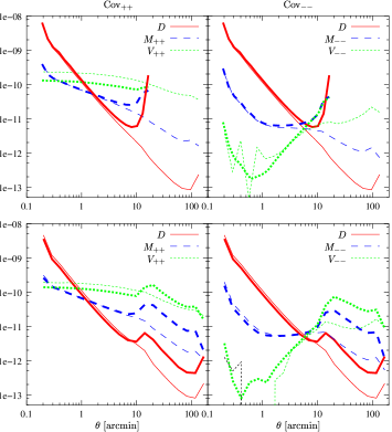
The covariance matrices of the correlation functions consist of three different terms: a shot noise term ($D$) which appears only on the diagonal and depends solely on the intrinsic ellipticity dispersion, a term which depends on cosmic variance only ($V$) and a mixed term ($M$). In Fig. 1, the diagonal elements of the covariance matrices are plotted, split up into the individual terms. For $\,\mbox{Cov}_{++}$, the cosmic variance $V$ dominates on scales larger than about one arc minute, whereas $\mbox{Cov}_{--}$ is dominated by $D$. As shown in the upper row of Fig. 1, there is about a factor of two in $V_{++}$ between the two extreme geometries regarding cosmic variance. The lower row of panels of Fig. 1 compares patch geometries with the same radius, but with a low ($N=10$) and a high ($N=60$) image density in the patches. In the first case, there is a sharp transition at the image boundary scale, which is not present for the denser patches.

4 Analysis

4.1 Maximum likelihood

Using the covariance matrices, we construct a figure-of-merit

$$\chi^{2}(p)\equiv\sum_{ij}\left(\xi_{i}(p)-\xi^{\rm t}_{i}\right)\mbox{Cov}_{ij}^{-1}\left(\xi_{j}(p)-\xi^{\rm t}_{j}\right),\;\;\;\;\;\;\;\xi_{i}\equiv\xi(\theta_{i}),$$ (3)

where the superscript ^t denotes the fiducial model (see Sect. 2) and $p$ is a set of cosmological parameters which is tested against this model. This figure-of-merit can be calculated using the two correlation functions $\xi_{+}$ and $\xi_{-}$ separately, or the combination of both; the resulting functions are called $\chi^{2}_{+}$, $\chi^{2}_{-}$ and $\chi^{2}_{\rm tot}$, respectively.

We calculated (3) for a number of different survey geometries. The most interesting constraints on cosmological parameters from cosmic shear are those on $\Omega_{\rm m}$ and $\sigma_{8}$. We kept all other parameters fixed and reparametrized $\sigma_{8}$ to $\Sigma_{8}\equiv\sigma_{8}/[0.41+0.59\left(\Omega_{\rm m}/0.3\right)^{-0.68}]$ in order to compensate for the high elongation of the $\Omega_{\rm m}$-$\sigma_{8}$- likelihood contours.

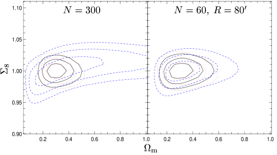
In Fig. 2, the $\Omega_{\rm m}$-$\Sigma_{8}$-likelihood contours of (3) are plotted, for two extreme geometrical configurations regarding cosmic variance: the uncorrelated images and the $(N=60,R=80^{\prime})$-patch geometry. Clearly, the $\chi^{2}_{-}$-contours are more extended in the case of the uncorrelated images than for the patch geometry. This is because $\xi_{-}$ contains much information on large scales which is absent in the case of the uncorrelated images. In contrast, the $\chi^{2}_{+}$-contours are tighter in this case than for the patch geometry.

Furthermore, in both cases, the difference between $\chi^{2}_{+}$ and $\chi^{2}_{\rm tot}$ are small. Thus, most of the information concerning these two cosmological parameters is contained in $\xi_{+}$; the additional information coming from $\xi_{-}$ is relatively small.

Figure 2: 1-$\sigma$, 2-$\sigma$ and 3-$\sigma$ confidence contours of the figure-of-merit (3). The parameter $\Sigma_{8}$ is proportional to $\sigma_{8}$, see text. Solid lines are from the combination of $\xi_{+}$ and $\xi_{-}$, dotted (dashed) lines are calculated using $\xi_{+}$ ($\xi_{-}$) alone. The left panel shows the results for the 300 uncorrelated images, the right panel is for a $(N=60,R=80^{\prime})$-patch geometry.

Figure 3: 1-$\sigma$-likelihood contours (solid lines) compared with the 1-$\sigma$-error ellipse from the Fisher matrix: the dashed ellipse is for a flat Universe (as it is the case for the likelihood contours), the dotted one is for $\Omega_{\Lambda}=0.7$. a/b is the axis ratio of the ellipses (the case $\Omega_{\Lambda}=0.7$ is in parentheses). The configuration is a survey of 300 uncorrelated images, we used the combined $\xi_{+}$ and $\xi_{-}$.

4.2 Fisher information matrix

The Fisher information matrix $F$ is defined as the expectation value of the second derivative of the likelihood function. From the Cramér-Rao inequality, we get a minimum variance bound (MVB) $\sigma(p_{i})=\sqrt{(F^{-1})_{ii}}$ for any unbiased estimator of a parameter $p_{i}$.

In Fig. 3, we compare the MVB from the Fisher matrix with the 1-$\sigma$-contours of the likelihood, using $\xi_{+}$ in both cases. As expected, the likelihood contours are larger than the 1-$\sigma$-ellipse from the Fisher matrix. The orientation of the Fisher ellipse coincides with the likelihood shapes, i.e. the direction of the minimal and maximal degeneracy of parameters is recovered. The larger the degeneracy between two parameters, the larger is the deviation between the local approximation by the Fisher matrix and the likelihood function.

Next, we assume that the parameters $\Omega_{\rm m},\sigma_{8},\Gamma$ and $n_{\rm s}$ are to be determined simultaneously from the survey and calculate the MVB for these parameters, using different survey geometries. We now perform the analyses using the ${M_{\rm ap}}$-statistics which is thought to be the most useful statistics for cosmic shear because of its ability to separate E- from B-modes.

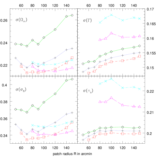
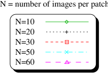
The MVB for these parameters for a variety of survey geometries is plotted in Fig. 4. The smallest values for the MBVs are obtained for a configuration with $N=30$ and $R=60^{\prime}-70^{\prime}$. Note the similarity of the curves for $\Omega_{\rm m}$ and $\sigma_{8}$ which both determine more or less the amplitude of the power spectrum, and those for $\Gamma$ and $n_{\rm s}$ which are responsible for the shape.

Figure 4: The MVB for the parameters $\Omega_{\rm m},\Gamma,\sigma_{8}$ and $n_{\rm s}$, using the $\left\langle M_{\rm ap}^{2}\right\rangle$-statistics. $\Omega_{\rm m},\Gamma,\sigma_{8}$ and $n_{\rm s}$ are assumed to be determined from the data, all other parameters are kept fixed. Each point in the plot represents a patch geometry with $N$ images in patches of radius $R$.

5 Conclusions

The best constraints on cosmological parametes are obtained for a survey with $N=30$ images distributed in patches on the sky. The dependence on the patch radius is quite small. The MVBs of some combinations of cosmological parameters to be determined from a cosmic shear survey with $N=30$ and $R=60^{\prime}$ are given in Table 2. The cosmological constant is only poorly constrained. For $\Omega_{\rm m},\sigma_{8},\Gamma$ and $n_{\rm s}$, the optimal survey consists of small patches of about $R=60$ arc minutes of radius, with $N=30$ images randomly distributed in each patch. The difference of the MVB makes up to 25 percent for different survey geometries, thus a 25 percent improvement on the determination on cosmological parameters can be obtained solely by choosing the appropriate survey geometry.

Table 2: Each row shows the MVBs for a combination of three or four cosmological parameters which are to be determined simultanously from a cosmic shear survey.

$\Omega_{\rm m}$	$\sigma_{8}$	$\Gamma$	$\Omega_{\Lambda}$	$n_{\rm s}$
0.18	0.28	0.04
0.20	0.28	0.10	0.41
0.22	0.34	0.15		0.20

Acknowledgements.  We thank Peter Schneider for useful discussions and helpful comments on the manuscript.

References

- [1] Réfrégier, A., “Weak Lensing by Large-scale Structure”, these proceedings
- [2] Kilbinger M. & Schneider P., 2003, A&A submitted, also astro-ph/0308119
- [3] van Waerbeke L., Mellier Y., Pelló R., Pen U.-L., McCracken H.J, Jain B., 2002, A&A 393, 369
- [4] Hoekstra H., Yee H.K.C., Gladders M.D. et al. 2002, ApJ 572, 55H
- [5] Jarvis M., Bernstein G.M., Fischer P., Smith D. 2003, AJ 125, 1014J
- [6] Réfrégier A., Rhodes J., Groth E.J. 2002, ApJL 572, L131
- [7] Maoli R., van Waerbeke L., Mellier Y., Schneider P., Jain B ., Bernardeau F., Erben T. & Fort B. 2001 A&A, 368, 766
- [8] Bardeen, J.M., Bond, J.R., Kaiser, N. & Szalay, A.S. 1986, ApJ, 304, 15
- [9] Peacock, J.A. & Dodds, S.J. 1996, MNRAS, 280, L19
- [10] Smail, I., Hogg, D. W., Yan, L., & Cohen, J. G. 1995, ApJL, 449, L105