Search for Global Dipole Enhancements in the HiRes-I Monocular Data above eV
Abstract
Several proposed source models for Ultra-High Energy Cosmic Rays (UHECRs) consist of dipole distributions oriented towards major astrophysical landmarks such as the galactic center, M87, or Centaurus A. We use a comparison between real data and simulated data to show that the HiRes-I monocular data for energies above eV is, in fact, consistent with an isotropic source model. We then explore methods to quantify our sensitivity to dipole source models oriented towards the Galactic Center, M87, and Centaurus A.
keywords:
cosmic rays , anisotropy , galactic center , Centaurus A , M87 , dipolePACS:
98.70.Sa , 95.55.Vj , 96.40.Pq , 13.85.Tp1 Introduction
The observation of Ultra-High Energy Cosmic Rays (UHECRs) has now spanned over forty years. Over that period, many source models have been proposed to explain the origin of these remarkable events. In the past five years, theoretical models have been suggested that would potentially produce dipole distributions oriented towards M87 [1] or Centaurus A [2, 3]. In addition, the Akeno Giant Air Shower Array (AGASA) has reported findings suggesting a 4% dipole-like enhancement oriented towards the Galactic Center present in its events with energies around eV [4]. This result seemed to be corroborated by findings published by the Fly’s Eye experiment in 1999 that suggested the possibility of an enhancement in the galactic plane also at energies around eV [5], and also by a re-analysis of data from the SUGAR array that was published in 2001 [6] that showed an enhancement in the general vicinity of the Galactic Center.
However, both AGASA and Fly’s Eye are subject to a limiting factor; they are both located too far north in latitude to directly observe the Galactic Center itself. The re-analysis of SUGAR data actually demonstrated an excess that was offset from the Galactic Center by and was more consistent with a point source than a global dipole effect [6]. While the current High Resolution Fly’s Eye (HiRes) experiment is subject to a similar limitation in sky coverage as the AGASA and Fly’s Eye experiments, we will show that, by properly estimating the HiRes aperture and angular resolution, we can effectively exclude these dipole source models to a certain degree of sensitivity. However, we are not able to completely exclude the findings of AGASA or the theoretical predictions mentioned above.
Our methods for detecting the presence of a dipole source model will be based upon comparisons between the real data and a large quantity of events generated by our Monte Carlo simulation program. The simulated data possess the same aperture and exposure as the actual HiRes-I monocular data set. In order to measure the presence of a dipole effect in our event sample, we use first a conventional binning technique that considers the event counts for the full range of opening angles from the center of each proposed dipole distribution. We then show how the asymmetric angular resolution of a monocular air fluorescence detector can be accommodated in this method. We ascertain the 90% confidence interval for a dipole source model for each of the three dipoles considered by comparing our real data with large numbers of similar-sized simulated data sets. We then consider the effects of systematic uncertainties on our measurements. To conclude, we use a novel technique measuring the information dimension [7], , of our sample to place an independent 90% confidence interval on the scaling parameter, , that we use to quantify our dipole source model.
2 The Dipole Function
A dipole source model can be described, as first proposed by Farrar and Piran [2]:
| (1) |
where is the relative density of cosmic rays in a given direction, is the opening angle between that direction and the global maximum of the distribution, and is the customary anisotropy amplitude [8]:
| (2) |
The cases of and correspond to 100% dipole distributions in the direction of the center and anti-center of the dipole source model, respectively. The case of corresponds to an isotropic source model.
A simple scheme for measuring consists of constructing a dipole function in the following manner:
-
1.
The opening angle is measured between the arrival direction of an event and the center of the proposed dipole source model.
-
2.
The cosine of the opening angle is then histogrammed.
-
3.
The preceding steps are repeated until all of the events are considered.
-
4.
The resulting curve produced by the histogram is the dipole function.
The dipole function has two variable parameters: the bin width, , and the total number of counts in all of the bins. At first glance, it would seem that the total bin count is fixed upon the total number of events, but we will show that this isn’t necessarily the case when we consider how to accommodate angular resolution.
In the simplest case of a sample that contains a very large number of events with a constant exposure and aperture over the entire sky, the dipole function will be proportional to equation 1. We propose two simple ways that one can quantify the dipole function for this sample; the most obvious way is to consider its slope. We can see by referring to equation 1 that this is equal to . A second way of quantifying is to consider the mean cosine value, for the dipole function:
| (3) |
Both methods of quantification produce values that are dependent upon . While the dependence of is linear in for the case of homogeneous full-sky coverage, we will find that this is not necessarily the case when considering the cumulative exposure of a ground-based air fluorescence detector.
3 Calculating the Dipole Function for the HiRes-I Monocular Data
We now consider the real data sample consisting of events that were included in the HiRes-I monocular spectrum measurement [9, 10]. This set contains 1526 events observed between May 1997 and February 2003 with measured energies greater than eV. The HiRes monocular data set represents a cumulative exposure of kmsryr at eV.
(a)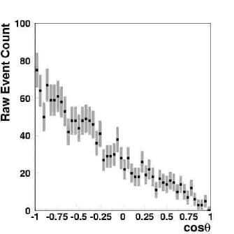
|
(b)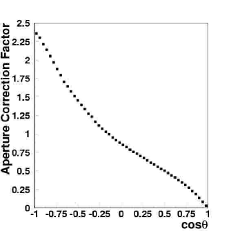
|
(c)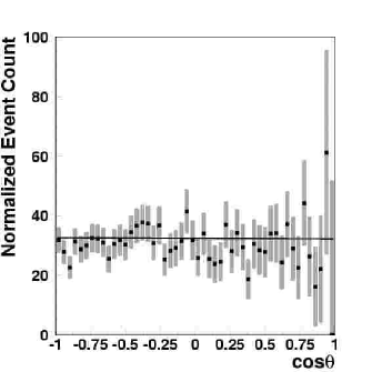
|
As a first order measurement, we construct the dipole function for a source model with a maximum value at the Galactic Center. For now, we only consider the nominal arrival directions of the events in our data sample. For this demonstration, we set the bin width of the dipole function to . This provides us with a mean bin count of 30.52. Figure 1a shows the resulting dipole function. However, in order to estimate the value of , we first normalize our dipole function with respect to aperture and exposure. This is done by considering pairs of simulated events and event times that correspond to the actual HiRes-I observation periods. By constructing a dipole function for this simulated set, we then estimate the normalization factor for each bin in the dipole function. The result is shown in figure 1b. The dipole function is then normalized and a -fit performed to determine its slope, , and -intercept, . The normalized dipole function is pictured in figure 1c with the best linear fit applied. The scaling constant, , is then estimated by the quotient, . The result for the galactic dipole source model is then: .
The same method was employed to calculate in the cases of Centaurus A and M87. For Centaurus A, we obtained a result of: . For M87, we found .
4 Incorporating Angular Resolution into the Dipole Function
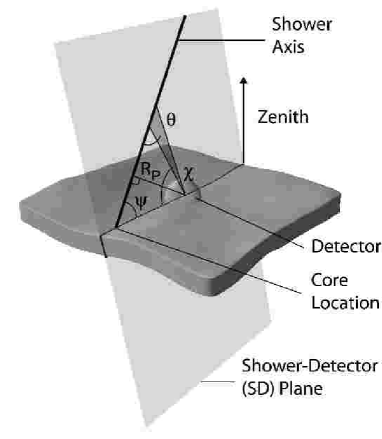
The analysis described in the previous section does not take into account the experimental angular resolution. Accommodating the angular resolution is important to the overall integrity of this analysis because the HiRes-I monocular data contains very asymmetric errors in arrival direction determination. For a monocular air fluorescence detector, angular resolution consists of two components, the error, in the estimation of the plane of reconstruction and the error, , in the determination of the angle, , within the plane of reconstruction. Figure 2 illustrates how this geometry would appear with a particular plane of reconstruction and a particular value for . Intuitively, we can see that the plane of reconstruction can be determined quite accurately. However, the value of is more difficult to determine because it is dependent on the precise results of the profile constraint fit [9, 10]. In general, is dependent upon the observed angular track length of the event in question. This is because longer track lengths enable a better determination of the plane of reconstruction. Typically, the value of is . The value of is dependent upon the cosmic ray energy. This is due to the fact the larger showers provide better defined profiles for the reconstruction program. Typically, the value of is .
 |
In order to accommodate the HiRes-I monocular angular resolution, it is necessary to revise the method we use to construct the dipole function. Instead of considering each event as a single arrival direction, we will consider each event to be an elliptical, two-dimensional Gaussian distribution of points with the two Gaussian parameters, and , being defined by the parameters that describe the angular resolution. Figure 3 shows how entire sets of events with these error parameters appear when projected on a density plot using a Hammer-Aitoff projection and equatorial coordinates.
(a)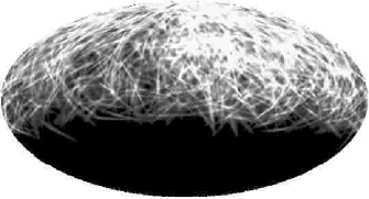
|
(b)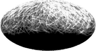
|
(c)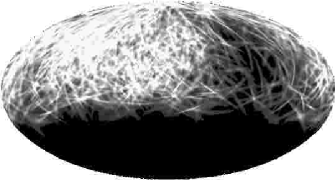
|
(d)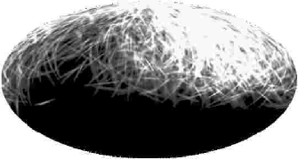
|
In order to account for angular resolution in the construction of the dipole function, we add an additional step. Instead of simply calculating the opening angle between the arrival direction of the event and the center of the dipole for the preferred arrival direction, we do so separately for each of the points in the Gaussian distribution that describes each event’s arrival direction. By choosing a sufficiently large value for and a sufficiently small bin width, , we can then construct the dipole function as a smooth curve. Examples of the dipole function are shown in figure 4 for each of the four event sets in figure 3.
(a)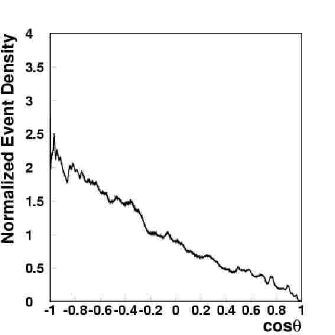
|
(b)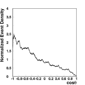
|
(c)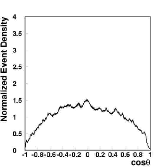
|
(d)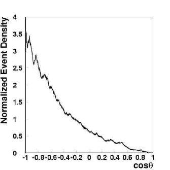
|
The next logical step would be to attempt to normalize the dipole function of the real data with respect to aperture and exposure and then to calculate the slope, , and the -intercept, . However, this program would run into a major complication. Because the Gaussian distributions that are used to approximate the individual event arrival directions can overlap into a large number of bins, the individual data points in the dipole function are highly correlated. This makes it impossible to apply either the -fit or a bootstrap method to estimate the error in the values of and —and thus the error in —for the normalized dipole function. Another approach needs to be developed.
The method that we propose is to compare the value of for the dipole function of the real data sample with that of a large number of similar-sized simulated data samples with a discrete spectrum of -values. We can then show how varies with respect to for different dipole source models.
5 Simulating the HiRes Aperture and Exposure
In creating simulated data sets, we employed a library of simulated events generated by our Monte Carlo shower simulation program and then reconstructed using the profile-constraint reconstruction program. This library of events possesses the spectrum and composition reported by the stereo Fly’s Eye experiment[11, 12]. A total of simulated events were reconstructed with energies greater than eV.
Once a library of simulated events was created, we then turned to the task of creating simulated data sets that accurately reflected the exposure of the HiRes-I monocular data set. In general, the apertures of air-fluorescence detectors are complicated; we need to assign times to individual Monte Carlo events that accurately reflect the distribution of times seen in the actual data.
By parsing through the raw HiRes-I data, we assemble a database of detector run-periods. We then randomly assign a time from these periods to each simulated event for a simulated event set. We also apply a further correction to account for the effect of non-functioning detector units (mirrors). This is achieved by excluding mirror events corresponding to periods in which a particular mirror was out of commission.
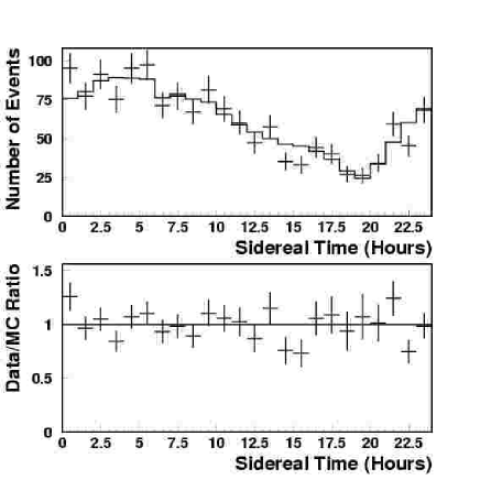
In figure 5 we can see the results of this mirror-by-mirror correction by comparing the sidereal time distributions of real and simulated data sets after the correction is applied. We see excellent agreement in this plot ().
 |
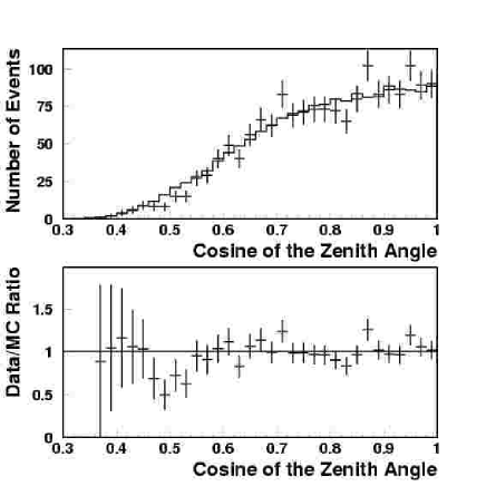
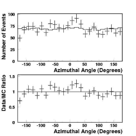
We also checked to see if the Monte Carlo shower simulation routine was accurately modeling the efficiency of the HiRes-I detector with respect to zenith and azimuth angles. In figures 6 and 7, we compare the distributions of zenith and azimuth angles for the real data and the simulated data set that has been assigned random times and filtered through our mirror-by-mirror correction. There is again very good agreement between the simulation and the data.
 |
 |
6 Results
For each of the three dipole source models considered we used the following procedure to measure the parameter:
-
1.
We calculated the value of for the dipole function of the real data sample.
-
2.
We created a total of 20,000 simulated data samples, 1000 each for 0.1 increments of from -1.0 to 1.0, each with the same number of events as the actual data. In figure 8 we can see that the distribution of values for each -value generated conforms well to a Gaussian distribution.
-
3.
We constructed curves corresponding to the mean and standard deviation of of the dipole function for each value of .
-
4.
We determined the preferred value of and the 90% confidence interval of for each dipole source model by referring to the intersections of the 90% confidence interval curves with the actual value of for the dipole function of the real data.
(a)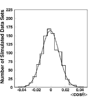
|
(b)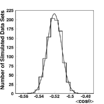
|
The results for all three dipole source models are shown in figure 9. In each case, the nominal values of and the 90% confidence levels only deviated marginally from the values obtained without considering angular resolution. The results are given in column 2 of table 1.
(a)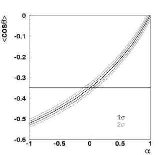
|
(b)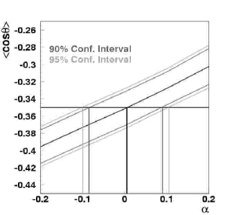
|
(c)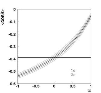
|
(d)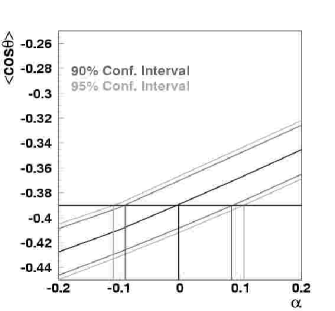
|
(e)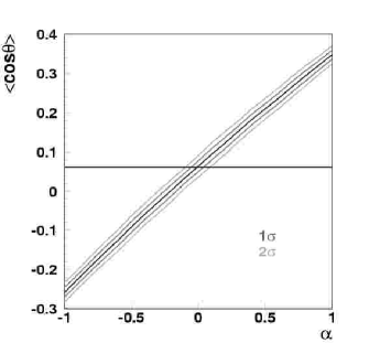
|
(f)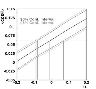
|
7 Potential Sources of Systematic Error in the Estimation of
There are two principal potential sources of systematic error in the determination of with HiRes-I monocular data. The first lies in the estimation of the angular resolution. If the error in arrival direction estimation was being underestimated or overestimated, it could lead to an improper evaluation of the confidence intervals for . In order to study the effect of angular resolution on our determination of , we repeated our analysis of the galactic dipole model twice. In the first case, we increased the estimated angular resolution parameters for both the real and simulated data sets by 33%. In the second case, we decreased the angular resolution parameters for both types of data sets by 25%. In both cases, the width of the 90% confidence interval for changed by less than 0.010 and the nominal value of remained unchanged. The results suggest that the determination of is largely independent of the angular resolution—at least for the plausible range of values that one could adopt for the angular resolution parameters.
The second issue of concern is the uncertainty in the determination of atmospheric clarity. Because hourly atmospheric observations are not available for the entire HiRes-I monocular data set, we have relied upon the use of an average atmospheric profile for the reconstruction of our data [13]. Different atmospheric conditions can influence how the profile constraint reconstruction routine interprets an observed shower profile and thus can lead to slightly divergent determinations of an event’s arrival direction. Unfortunately, we do not have large libraries of simulated data with differing atmospheric parameters used in the generation and reconstruction of events. However, we do have the real data reconstructed with a full range of atmospheric parameters. By considering the value of over the error space of atmospheric parameters, we can establish the degree of systematic uncertainty that is contributed to the determination of by atmospheric variability. We saw that in the most extreme case, the nominal value of shifted by less than . There was no broadening in the 90% confidence interval.
8 Using the Information Dimension, , as an Independent Check
The information dimension, [14, 15], is a measure of the overall heterogeneity of a data sample. The smaller the value of , the more heterogeneous the sample is. A basic formula for calculating is:
| (4) |
where is the total number of declinational bins (with a range of values between 354 to 360) and:
| (5) |
with being the number of counts in a particular latitudinal bin, being the average bin count over the entire sample and being the area of that particular latitudinal bin. A detailed description of this method can be found in reference [7].
While the measurement of is not necessarily the most sensitive tool available, it allows one to rule out any number of potential anisotropic source models with a single measurement. The general scheme that we followed is similar to what we used in the case of the dipole function.
-
1.
We calculated the value of for the real data sample.
-
2.
We created a total of 20,000 simulated data samples, 1000 each for 0.1 increments of from -1.0 to 1.0. In figure 10 we can see that distribution of values for each -value is Gaussian.
-
3.
We constructed a curve consisting of the mean and standard deviation of for each value of .
-
4.
We then ascertained the preferred value of and the 90% confidence interval for each dipole source model by referring the intersections of the 90% confidence interval curves with the actual value of for the real data.
(a)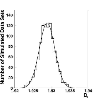
|
(b)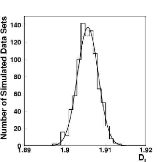
|
The results for all three dipole source models are shown in figure 11.
(a)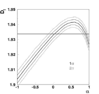
|
(b)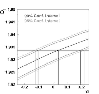
|
(c)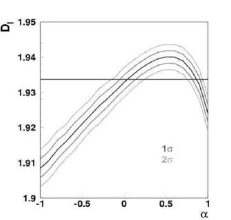
|
(d)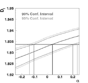
|
(e)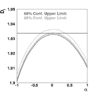
|
(f)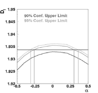
|
The determination of for both methods are compared in Table 1. The 90% confidence intervals for the determination via the use of are substantially larger. This is to be expected because the value of is a single number that contains no a priori preference for a specific source model. Furthermore, in two cases there is a second solution to that is excluded by considering the results of the method. The important observation is that the results of the two methods are consistent. One advantage of the method is that we can state all three 90% confidence intervals jointly, since they are all considering only a single measurement on the real data. In the case of the method, we would have to consider a broader confidence interval for each individual model in order to have a simultaneous 90% confidence level for all three models.
| 1 | 2 | 3 | |
| determined | determined | determined | |
| SOURCE MODEL | without considering | by the value of | by the value of |
| angular resolution | |||
| Galactic | |||
| Centaurus A | |||
| M87 |
9 Conclusion
We are able to place upper limits on the value of for each of our three proposed dipole source models. However, these limits are not small enough to exclude the theoretical predictions [1, 2, 3]. Also, they do not exclude the findings of the AGASA collaboration in terms of the intensity of the dipole effect that they observed or in terms of the energy considered because the events in the dipole effect observed by the AGASA detector possessed energies below eV [4]. Since it appears that angular resolution has little impact on the measurement of and we do not appear to be systematically limited, we conclude that the driving factor in making a better determination of will simply be larger event samples. HiRes-I mono will continue to have the largest cumulative aperture of any single detector for the next three to five years, thus it will continue to serve as an ever more powerful tool for constraining dipole source models.
10 Acknowledgments
This work is supported by US NSF grants PHY 9322298, PHY 9321949, PHY 9974537, PHY 0071069, PHY 0098826, PHY 0140688, PHY 0245428, by the DOE grant FG03-92ER40732, and by the Australian Research Council. We gratefully acknowledge the contributions from the technical staffs of our home institutions. We gratefully acknowledge the contributions from the University of Utah Center for High Performance Computing. The cooperation of Colonels E. Fisher and G. Harter, the US Army and the Dugway Proving Ground staff is appreciated.
References
- [1] P. L. Biermann, E. J. Ahn, G. Medina Tanco and T. Stanev, Nucl. Phys. Proc. Suppl. 87, 417 (2000) [arXiv:astro-ph/0008063].
- [2] G. R. Farrar and T. Piran, arXiv:astro-ph/0010370.
- [3] L. A. Anchordoqui, H. Goldberg and T. J. Weiler, Phys. Rev. Lett. 87, 081101 (2001) [arXiv:astro-ph/0103043].
- [4] N. Hayashida et al. [AGASA Collaboration], arXiv:astro-ph/9906056.
- [5] D. J. Bird et al. [HIRES Collaboration], arXiv:astro-ph/9806096.
- [6] J. A. Bellido, R. W. Clay, B. R. Dawson and M. Johnston-Hollitt, Astropart. Phys. 15, 167 (2001) [arXiv:astro-ph/0009039].
- [7] B. T. Stokes, C. C. H. Jui and J. N. Matthews, arXiv:astro-ph/0307491.
- [8] P. Sommers, Astropart. Phys. 14, 271 (2001) [arXiv:astro-ph/0004016].
- [9] T. Abu-Zayyad et al. [High Resolution Fly’s Eye Collaboration], arXiv:astro-ph/0208243.
- [10] T. Abu-Zayyad et al. [High Resolution Fly’s Eye Collaboration], arXiv:astro-ph/0208301.
- [11] D. J. Bird et al. [HIRES Collaboration], Astrophys. J. 424, 491 (1994).
- [12] D. J. Bird et al. [HIRES Collaboration], Proc. of 23rd ICRC (Calgary), 2, 38 (1993).
- [13] L. R. Wiencke et al. [HIRES Collaboration], Proc. of 27th ICRC (Hamburg), 1, 635 (2001).
- [14] J. Balatoni and A. Reyni, Publ. Math. Inst. Hung. Acad. Sci. 1, 9 (1959).
- [15] A. H. Nayfeh and B. Balachandran, Applied Nonlinear Dynamics: Analytical, Computational, and Experimental Methods (Wiley, New York, 1995) pp. 545-547.