Mass and redshift dependence of dark halo structure

Abstract

Using a combination of N-body simulations with different resolutions, we study in detail how the concentrations of cold dark matter (CDM) halos depend on halo mass at different redshifts. We confirm that halo concentrations at the present time depend strongly on halo mass, but our results also show marked differences from the predictions of some early empirical models. Our main result is that the mass dependence of the concentrations becomes weaker at higher redshifts, and at $z\gtrsim 3$ halos of mass greater than $10^{11}{h^{-1}M_{\odot}}$ all have a similar median concentration, $c\sim 3.5$. While the median concentrations of low-mass halos grow significantly with time, those of massive halos change only little with redshifts. These results are quantitatively in good agreement with the empirical model proposed by Zhao et al. which shows that halos in the early fast accretion phase all have similar concentrations.

1 Introduction

High-resolution $N$-body simulations have shown that the density profiles of cold dark matter (CDM) halos can be described reasonably well by a universal form,

$$\rho(r)=\frac{4\rho_{s}}{(r/r_{s})\left(1+r/r_{s}\right)^{2}}\,,$$ (1)

where $r_{s}$ is a characteristic “inner” radius, and $\rho_{s}$ is the density at $r_{s}$ (Navarro, Frenk and White 1996, 1997; NFW hereafter), although there is still debate about the exact value of the inner slope (e.g. Fukushige & Makino 1997, 2003; Moore et al. 1998; Jing & Suto 2000). For a halo of radius $R$, this profile is characterized by the concentration parameter $c=R/r_{s}$, which is found to be dependent on halo mass (smaller halos have, on average, higher concentrations). NFW developed a simple model to account for this mass dependence. The NFW model for the mass dependence of $c$ was later found to be inconsistent with results obtained from a simulation of the concordance low-density CDM model (LCDM) at high redshift (Bullock et al., B01 hereafter). B01 found that $c$ is proportional to the cosmic scale factor $a$ for a given halo mass. Based on this, B01 and Eke et al. (2001; E01 hereafter) proposed new empirical prescriptions to predict $c$ as a function of redshift and halo mass.

It must be noticed, however, that all these prescriptions only give the mean concentration of all halos of a given mass at a given redshift. Since the density profiles are found to vary significantly from one halo to another even for a given halo mass (Jing 2000; B01), it is important to have a recipe to predict $c$ for individual halos. Jing has examined the density profiles for halos in different dynamical states, and found that the halo density profiles are closely related to the halo formation history. The connection between halo concentration and halo formation history was explored further by Wechsler et al. (2002; W02). Assuming that $c=4.1$ at their defined “formation redshift” and $c\propto a$, W02 found that their model prediction for $c$ is in good agreement with their simulation results for the LCDM model.

In a recent paper, Zhao et al. (2003; hereafter ZMJB) found that, for a given halo, there is a tight correlation between the inner scale radius $r_{s}$ and the mass within it, $M_{s}$, for all its main progenitors, and that this correlation can be used to predict the concentration of a dark halo at any time without making any ad hoc assumption about the form of the mass accretion history. The ZMJB model predicts that the evolution of $c$ of individual halos are not just a function of $a$ (such as $c\propto a$ as W02 assumed), but tightly connected to their mass growth rate: the faster the mass grow, the slower the $c$ increase.

In this Letter we use a combination of high-resolution simulations of different boxsizes to directly explore the halo structures for a wide range of halo mass in a wide range of redshifts. This allows us to study in detail how halo concentration depends on halo mass at various redshifts, and to test the accuracy of the various empirical models mentioned above. We will show that at high redshift the simulated mass dependence of $c$ is much different from some previous results, and is quantitatively in good agreement with ZMJB prediction.

2 Simulation results

The cosmological simulations used in this paper are generated with a parallel-vectorized Particle-Particle/Particle-Mesh code (see Jing & Suto 2002). The concordance CDM model with the density parameter $\Omega_{0}=0.3$ and the cosmological constant $\lambda_{0}=0.7$ is considered. The linear power spectrum has the shape parameter $\Gamma=\Omega_{0}h=0.20$ and the amplitude $\sigma_{8}=0.9$, where $h$ is the Hubble constant in $100\,{\rm{km\,s^{-1}}}\hbox{\rm Mpc}^{-1}$, and $\sigma_{8}$ is the rms top-hat density fluctuation within a sphere of radius $8\,h^{-1}{\rm{Mpc}}$ at the present time. We use $256^{3}$ particles for the simulation of boxsize $L=25\,h^{-1}{\rm{Mpc}}$, and $512^{3}$ particles for the other two simulations of $L=100$ and $300\,h^{-1}{\rm{Mpc}}$ (Table 1). The simulations with $L=25\,h^{-1}{\rm{Mpc}}$ and $100\,h^{-1}{\rm{Mpc}}$ have been evolved by 5000 time steps with a force softening length $\eta$ (the diameter of the S2 shaped particles, Hockney & Eastwood 1981) equal to $2.5h^{-1}{\rm kpc}$ and $10h^{-1}{\rm kpc}$, respectively. As a result, there are many halos with more than $3000$ particles in these simulations, and these halos are resolved similarly to or better than the individual halo simulations in early studies of the density profiles (e.g. NFW). It has been shown that the resolution at this level is sufficient for determining the concentration parameter (Jing 2000; E01), though it may not be good enough for addressing the issues with regard to the slope of the density profile in the central region of a halo (e.g. Fukushige & Makino 1997, 2003; Moore et al. 1998; Jing & Suto 2000). The simulation of $L=300\,h^{-1}{\rm{Mpc}}$ is a typical cosmological simulation, evolved by 1200 steps and with a force softening length of $30h^{-1}{\rm kpc}$. The halo sample constructed from these simulations is big, which is essential for accurately determining the mean halo concentration. There is a sufficient overlap in mass between the halos of different simulations, from which the resolution effect can be reliably estimated. The halos are defined according to the spherical virialization criterion (Kitayama & Suto 1996; Bryan & Norman 1998), so the radius $R$ of a halo in this paper is the virial radius $r_{\rm vir}$. The halos are identified from simulations using the potential minimum method as described in Jing & Suto (2002), and the particle with the minimum potential in each halo is chosen as the halo center. We use all halos identified this way without applying any further selection criteria.

Table 1: A summary of simulation parameters

simulation	$N_{\rm p}$	box size	$M_{\rm part}$	$\eta$	$z_{\rm initial}$
		$\,h^{-1}{\rm{Mpc}}$	${h^{-1}M_{\odot}}$	$\,h^{-1}{\rm{kpc}}$
LCDM025	$256^{3}$	25	$8.0\times 10^{7}$	2.5	72
LCDM100	$512^{3}$	100	$6.4\times 10^{8}$	10	72
LCDM300	$512^{3}$	300	$1.7\times 10^{10}$	30	36

2.1 The mass accretion history

Following ZMJB, we construct the main branch of the merger tree for each halo identified at redshift $z=0$, and work out the mass accretion history. In Figure 1, we plot the mass accretion histories for 20 randomly selected halos at each of the following mass scales: $M_{\rm vir,0}=7\times 10^{10}{h^{-1}M_{\odot}}$, $1.3\times 10^{13}{h^{-1}M_{\odot}}$, and $1.4\times 10^{15}{h^{-1}M_{\odot}}$. As in ZMJB, the mass accretion history of each halo is divided into a fast accretion phase and a slow accretion phase, and we denote the transition redshift between the two by $z_{tp}$. With the mass $M_{\rm vir}(z)$ in units of $M_{\rm vir,tp}=M_{\rm vir}(z_{\rm tp})$ and the physical virial density $\rho_{\rm vir}(z)$ in units of $\rho_{\rm vir,tp}=\rho_{\rm vir}(z_{\rm tp})$ , we found that the mass accretion history has a universal form for halos of different mass, and the mean accretion history can be accurately represented by the thick smooth line for the halo masses covered by the simulations (from $7\times 10^{10}{h^{-1}M_{\odot}}$ to $1.3\times 10^{15}{h^{-1}M_{\odot}}$). Mathematically, the average accretion history can be expressed in the form:

$${M_{\rm vir}(z)\over M_{\rm vir,tp}}={x^{0.3}\over 1-a+ax^{-1.8a}}\,,$$ (2)

where $x=\rho_{\rm vir,tp}/\rho_{\rm vir}(z)$ and $a=0.75$ ($0.42$) for the fast (slow) accretion phase. The universal mass history has interesting implications for galaxy formation and halo structure formation. Here because of the limited space, we will only discuss its implications for halo structure in §3.

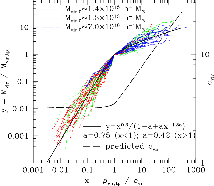
Figure 1: The mass accretion history of dark matter halos along the main branch. Twenty halos are randomly selected from the simulations at each mass indicated at the top. We use the physical density within the virialized halo $\rho_{\rm vir}(z)$ as the time variable. Both the halo mass $M_{\rm vir}(z)$ and $\rho_{\rm vir}(z)$ are scaled to their quantities at the turning point, $M_{\rm vir,tp}$ and $\rho_{\rm vir,tp}$. The scaled mass accretion history on average is well represented by Eq.(2) independent of the halo mass. The thick smooth dashed line is the prediction of ZMJB for the concentration $c_{\rm vir}$ according to the mean accretion history (the right vertical coordinate for $c_{\rm vir}$).

2.2 Halo concentrations

We select halos with more than $800$ particles at redshifts $z=0$, $1$, $2$ and $4$, and determine the concentration parameter for each of them by fitting the density profile to the NFW form (see ZMJB for the fitting procedure). The halos are grouped in mass bins of $\Delta\log_{10}M_{\rm vir}=0.2$, and the median concentration is calculated for each mass bin. The median concentrations determined this way are presented in Figure 2 for masses larger than $6.4\times 10^{10}{h^{-1}M_{\odot}}$, together with their errorbars (standard deviation among different halos in the bin divided by the square root of the halo number). Note that there is always quite a large overlap in halo mass between simulations of different boxsizes, and that the median concentrations from different simulations are in good agreement in the overlapping mass range. This agreement suggests that our results are not significantly affected by the finite numerical resolution, because for a given halo mass both the mass and force resolutions decrease with the increase of the simulation boxsize.

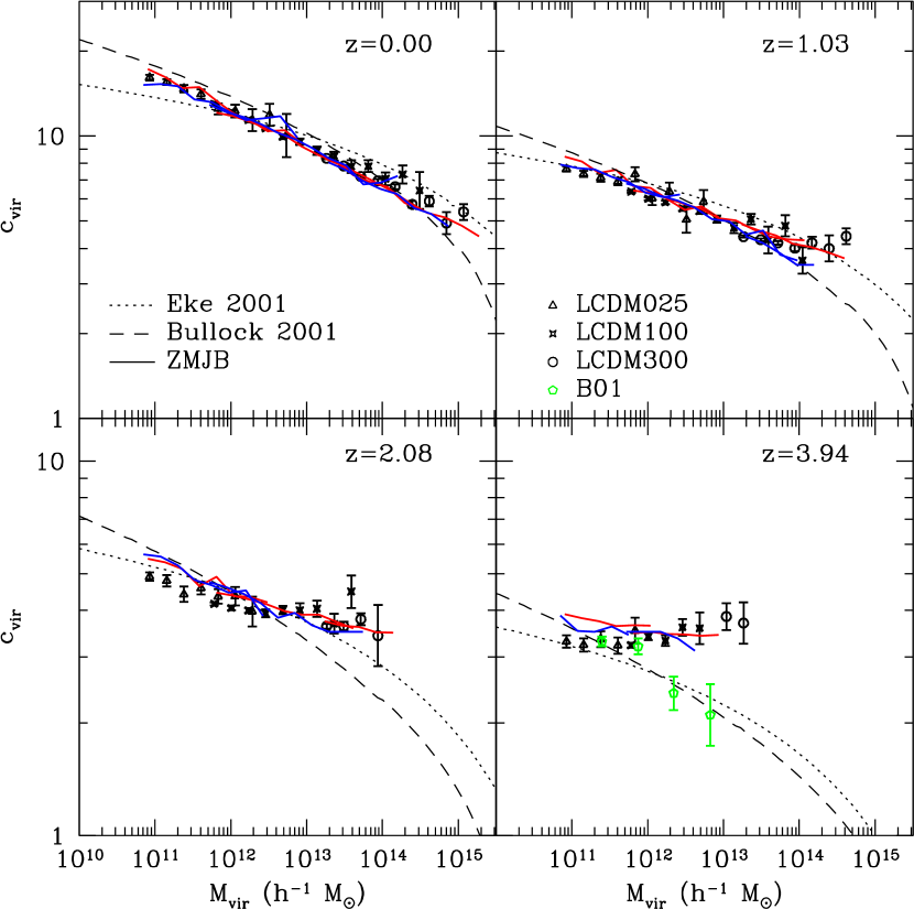
Figure 2: The median concentration of halos as a function of the halo mass. Errorbars are the standard deviation among halos of the same mass devided by square root of the halo number. The black symbols are for the results measured in the simulations, the blue and red lines are the predictions of ZMJB using the mass accretion histories from the simulations (blue) and from the PINOCCHIO model (red), and the dashed and dotted lines are the predictions of the models of Bullock et al. and Eke et al., respectively. For comparison, the simulation results of Bullock et al. for $z=4$ are plotted in the lower right panel as green pentagons.

As one can see, at low redshift, the median concentration decreases rapidly with halo mass, from $c\sim 20$ for $M_{\rm vir}\sim 10^{11}{h^{-1}M_{\odot}}$ to $c\sim 4$ for $M_{\rm vir}\sim 10^{15}{h^{-1}M_{\odot}}$. This mass dependence is similar to that found in earlier analyses (e.g. NFW; Jing & Suto 2000; B01 ). The mass dependence is weaker for halos at higher redshifts and becomes insignificant at $z\gtrsim 3$. This change in behavior is mainly due to the fact that the median concentrations of small halos decrease rapidly with increasing redshift while the concentrations of massive halos change little. Note that the decrease of $c$ with $z$ is slower at higher $z$ and there seems to be a minimum value $c\sim 3$ for the median concentration of dark halos. This is true even for a few halos at $z\sim 9$ that are not included here.

3 Comparison with empirical models

Based on results from numerical simulations, ZMJB found that the scale radius $r_{s}$ of a halo and its scale mass $M_{s}$ (i.e. the mass within $r_{s}$) are tightly correlated, with a relation well represented by a simple power law:

$${M_{s}\over M_{s,0}}=\left({r_{s}\over r_{s,0}}\right)^{3\alpha}\,,$$ (3)

where $M_{s,0}$ and $r_{s,0}$ are the scale mass and scale radius at some chosen epoch. The value of $\alpha$ is found to be $0.52$ in the slow accretion phase, and $0.64$ for the rapid accretion phase. As shown in ZMJB, this $M_{s}$-$r_{s}$ relation can be used to derive $c$ from the halo mass accretion history according to

$${[\ln(1+c)-c/(1+c)]c^{-3\alpha}\over[\ln(1+c_{0})-c_{0}/(1+c_{0})]c_{0}^{-3\alpha}}=\left[{\rho_{\rm vir}(z)\over\rho_{\rm vir,0}}\right]^{\alpha}\left[{M_{\rm vir}(z)\over M_{\rm vir,0}}\right]^{1-\alpha}\,.$$ (4)

This relation can be calibrated by fixing $c_{\rm tp}$ at $z=z_{tp}$. ZMBJ have calibrated $c_{\rm tp}$ with five high resolution halos, and adopted $c_{\rm tp}=4.0$. With our current large sample, we find $c_{\rm tp}=3.5$ to be more accurate.

With the universal mass accretion history obtained from our simulations, this recipe can be used to predict the median concentration as a function of redshift. The result is shown as the smooth dashed line in Figure 1. As one can see, the halo concentration has a value about $3.5$ in the fast accretion phase, and scales roughly as $c\propto\rho_{\rm vir}^{-1/3}(z)$ in the slow-accretion phase. This is consistent with our simulation results, that halos with masses between $10^{13}$ – $10^{14}{h^{-1}M_{\odot}}$ have median concentrations independent of $z$ at $z\gtrsim 1$. Most of these massive halos are in the fast accretion phase at these high redshifts. Note that the median concentration obtained from the simulations never drops below 3 even for the most massive halos at the highest redshift probed by our simulations, in agreement with the ZMJB model. The strong increase of $c$ with decreasing $z$ for low-mass halos at low redshift observed in the simulations is also consistent with the model prediction, because most of those halos are in their slow accretion phases.

We generate samples of mass accretion histories from the simulations, and apply the ZMJB model to predict the concentrations for each of these halos (Figure 2). The model prediction reproduces well the mass and redshift dependence of halo concentrations obtained from the simulations. The distribution of the concentrations for given halo mass and redshift is well described by the log-normal distribution with $\sigma_{\ln c}\approx 0.3$ (Jing 2000, B01). We also compute mass accretion histories using the PINOCCHIO code of Monaco et al. (2002). This code identifies dark matter halos and their merging histories by applying an ellipsoidal collapse model to an initial cosmic density field. It has been shown to be quite accurate in reproducing many properties of the halo population. All parameters are kept the same as in the simulaitons, and also we apply the ZMJB model to predict the halo concentrations. Again the agreement with our simulation results is satisfactory with an accuracy better than $10\%$ (Figure 2). In a forthcoming paper (Zhao et al., in preparation), we will show that the ZMJB prediction is valid for a wide range of cosmological models, including the SCDM model, an OCDM model, and scale-free models.

The increase of the halo concentration with decreasing redshift in the slow accretion phase is qualitatively consistent with the relation $c(M_{\rm vir},z)\propto(1+z)^{-1}$ found by B01, because $\rho_{\rm vir}(z)$ is approximately proportional to $(1+z)^{3}$. It is however important to note that the evolution we obtained is along the main branches of merger trees, while the relation $c(M_{\rm vir},z)\propto(1+z)^{-1}$ obtained by B01 is for the median concentration of a halo population of a given mass $M_{\rm vir}$. There is a marked difference of the prediction of the ZMJB model from that of B01: while ZMJB predicts that $c$ does not change in the fast accretion, B01 predicts $c\propto(1+z)^{-1}$ for a given mass.

In Figure 2, we compare our results to the predictions of the empirical models given by B01 and E01. The B01 model agrees with our simulation results well at redshift $z=0$ for $M_{\rm vir}\leq 10^{14}{h^{-1}M_{\odot}}$. Note that this is approximately the mass range that their simulation can effectively explore; their simulation uses $256^{3}$ particles in a box of $60\,h^{-1}{\rm{Mpc}}$. The B01 model also agrees with the redshift dependence of $c$ for low-mass halos, but it fails to match our simulation results at the high mass ends. The model of E01 fits our simulation data better for $z=1$ and $2$, but worse for $z=0$ than the B01 model. Since the Eke et al. model adopted a redshift-dependence of $c$ similar to that of B01 model, it also underestimates the concentration for massive halos at high redshift.

It should be pointed out that the models of B01 and E01 both match their own simulations to redshift $4$ and $2$, respectively, and so there seems to be a discrepancy among the different simulation results. Our results are consistent with the simlation results of E01 over the mass and redshift ranges probed by their simulations. Note that the very low concentrations obtained by E01 are for a warm dark matter spectrum. There is a marked difference between B01’s simulation results and ours for $z>2$; as comparison we plot in the low-right panel of Figure 2 their simulation results for $z=4$ (green pentagons). As one can see, the discrepancy between B01 and our simulation results becomes significant at $M_{\rm vir}\gtrsim 5\times 10^{12}{h^{-1}M_{\odot}}$ for this redshift. Unfortunately, the origin of this discrepancy is unknown. Our $100h^{-1}{\rm Mpc}$ box simulation has a mass resolution slightly better than their main ($60h^{-1}{\rm Mpc}$) simulation, and in terms of halo number, our sample is more than 4 times larger. Since the number density of massive halos is low at high $z$, and since halo concentration can differ substantially for halos with the same mass at the same redshift, a large sample might be crucial to get reliable results. We are confident about our results, because our halo sample is large and our simulations with different resolutions and boxsizes agree with each other very well.

As mentioned earlier, the consistency of the results obtained for different simulation boxsizes indicates that our determination of halo concentrations should not be affected significantly by the limited simulation resolution. As shown by Moore et al. (1998) and Diemand et al. (2003), the finite resolution should reduce the halo concentration. Comparing our results for different boxsizes, it appears that the resolution effect can lead to an underestimate of $c$ by $\lesssim 5\%$ at the lower halo mass end in each simulation. The slight systematic difference between the simulation results and the ZMJB model predictions may be caused by this resolution effect, and correcting for this may give a better agreement between the simulation data and model predictions. We have also examined the validity of the NFW profile for halos that are in the fast accretion phase, and found that most of these halos can be fitted by this profile (Zhao et al. in preparation).

4 Discussion and conclusions

We have studied the dependence on mass and redshift of the concentration of cold dark matter (CDM) halos in high resolution simulations, and discovered that at early times the mass dependence of halo concentrations which is pronounced at present, becomes insignificant, and at $z\gtrsim 3$ halos of mass $>10^{11}{h^{-1}M_{\odot}}$ have in the mean the same density profile with $c\sim 3.5$. Our results indicate that the median concentration of halos cannot decrease with redshift or/and halo mass to a value less than $\sim 3$. Massive cluster halos at present have higher concentrations than some previous models predicted.

The good agreement between the results of $c$ from different simulations demonstrates that the simulation resolution effect has been well controlled in our analysis.

For the mass accretion histories of halos with masses from $10^{10}$ to $10^{15}{h^{-1}M_{\odot}}$, we have found that they are well expressed by the universal function [Eq(2)].

All these results can be quantitatively matched by the empirical model of ZMJB. In that model the concentration of a halo is related to its mass accretion history through the scaling relation they found for $r_{s}$ and $M_{s}$. It predicts that all halos in the fast accretion phase have similar concentrations, regardless of their mass or their redshift . The ZMJB model reproduces our results both in the fast and the slow accretion phases. Since directly modelling halo density profiles in numerical simulations is both expensive and time consuming, the ZMJB model provides a practically useful technique for modeling internal structures of individual CDM halos.

While the model of Bullock et al. (B01) agrees with our results for halos in slow accretion, it seriously underestimates the concentration of halos in the fast accretion phase. The models of E01 have the same weakness as B01, since they all adopt a similar assumption that $c(M_{\rm vir},a)\propto a$.

The implications for galaxy formation models, and for the interpretation of observations, such as strong and weak lensing surveys, are interesting. According to our results, massive cluster halos at the present time, galactic halos at $z\sim 3$, and halos of the first collapsed objects in the universe at $z\sim 15$ (such as POP III stars) should all have about the same concentration.

References

- Bryan & Norman (1998) Bryan, G.L, & Norman, M., 1998, ApJ, 495, 80
- Bullock et al. (2001) Bullock, J. S., Kolatt, T. S., Sigad, Y., Somerville, R. S., Kravtsov, A. V., Klypin, A. A., Primack, J. R., & Dekel, A. 2001, MNRAS, 321, 559 (B01)
- Diemand et al. (2003) Diemand, J., Moore, B., Stadel, J., & Kazantzidis J. 2003, MNRAS, submitted (astro-ph/0304549)
- Eke, Navarro & Steinmetz (2001) Eke, V. R., Navarro, J.F., & Steinmetz, M. 2001, ApJ, 554, 114 (ENS)
- Fukushige & Makino (1997) Fukushige, T., & Makino, J. 1997, ApJ, 477, L9
- Fukushige & Makino (2003) Fukushige, T., & Makino, J. 2003, ApJ, 588, 674
- Hockney & Eastwood (1981) Hockney, R. W., & Eastwood, J. W. 1981, Computer Simulation Using Particles (McGraw Hill, New York)
- Jing (2000) Jing, Y. P. 2000, ApJ, 535, 30
- Jing & Suto (2000) Jing, Y. P., & Suto Y. 2000, ApJ, 529, L69
- Jing & Suto (2002) Jing, Y. P., & Suto Y. 2002, ApJ, 574, 538
- Kitayama & Suto (1996) Kitayama, T., & Suto, Y. 1996, MNRAS, 280, 638
- Monaco et al. (2002) Monaco, P., Theuns, T., Taffoni, G., Governato, F., Quinn, T., & Stadel, J. 2002, ApJ, 564, 8
- Moore et al. (1998) Moore, B., Governato, F., Quinn, T., Stadel, J., & Lake, G. 1998, ApJ, 499, L5
- Navarro, Frenk, & White (1996) Navarro, J. F., Frenk, C. S., & White, S. D. M. 1996, ApJ, 462, 563
- Navarro, Frenk, & White (1996) Navarro, J. F., Frenk, C. S., & White, S. D. M. 1997, ApJ, 490, 493
- Wechsler et al. (2002) Wechsler, R. H., Bullock, J. S., Primack, J. R., Kravtsov, A. V., & Dekel, A. 2002, ApJ, 568, 52
- Zhao et al. (2003) Zhao, D. H., Mo, H. J., Jing, Y. P., & Boerner, G. 2003, MNRAS, 339, 12 (ZMJB)