An Unsplit, Cell-Centered Godunov Method for Ideal MHD

Abstract

We present a second-order Godunov algorithm for multidimensional, ideal MHD. Our algorithm is based on the unsplit formulation of Colella (J. Comput. Phys. vol. 87, 1990), with all of the primary dependent variables centered at the same location. To properly represent the divergence-free condition of the magnetic fields, we apply a discrete projection to the intermediate values of the field at cell faces, and apply a filter to the primary dependent variables at the end of each time step. We test the method against a suite of linear and nonlinear tests to ascertain accuracy and stability of the scheme under a variety of conditions. The test suite includes rotated planar linear waves, MHD shock tube problems, low-beta flux tubes, and a magnetized rotor problem. For all of these cases, we observe that the algorithm is second-order accurate for smooth solutions, converges to the correct weak solution for problems involving shocks, and exhibits no evidence of instability or loss of accuracy due to the possible presence of non-solenoidal fields.

url]astron.berkeley.edu/$\sim$mookie/

Received 27 October 2003; accepted ***

1 Introduction

In this paper we present a new Godunov method for the equations of multidimensional ideal magnetohydrodynamics (MHD). We give results from an implementation of the unsplit, second-order method of Colella [10] for these equations. The base scheme solves the ideal MHD equations using a second-order predictor-corrector formalism. To the base scheme we add three algorithmic components, whose effects upon accuracy and stability are measured. The first component is a MAC projection [6, 19] step, which uses a Poisson solver to ensure that the cell-edge centered fields used to calculate fluxes are divergence-free to solver tolerance. This component, though commonplace in the context of incompressible Navier-Stokes simulation, is new to the MHD community. The second component is an approximate projection [2] that uses another solution of the Poisson equation to ensure that the cell-centered field is divergence-free to second-order. The last component is a filter [24] that also acts to suppress monopole sources in the cell-centered field.

The section that follows covers recent work and some of the schemes used for ideal MHD simulation. It also introduces methods for enforcing the divergence-free constraint, and introduces some issues surrounding multidimensional MHD. Section 3 introduces our basic algorithm and the extensions we have implemented. A suite of linear and nonlinear test problems will be used to determine which of our algorithmic extensions are best suited to each problem type. These tests and results are covered in Section 4. The overall purpose is to find one combination of these extensions that is well suited to all of the problems considered. This will be done through comparisons to published results and in some cases to an eight-wave MHD algorithm we have implemented. We find that a projection step is indeed required for accuracy and stability of the schemes. For the eight-wave scheme in particular, use of the MAC projection is essential to obtain correct MHD shock jumps.

2 Background

The study of numerical algorithms for magnetohydrodynamics simulations remains an active one, with no one method having become the standard. Two generic algorithms are the most widely used at present: the Method of Characteristics/Constrained Transport (MOC/CT; common in the astrophysics community) [15, 33] and shock-capturing (Godunov) methods [5, 9, 11, 12, 18, 30, 36, 39]. Each has distinct benefits and drawbacks. Codes implementing the MOC/CT algorithm are relatively simple in design, and satisfy the divergence-free constraint to machine precision. However, the method of characteristics used by the ZEUS scheme, as outlined in [33], is by construction second-order on Alfvén and advective waves, but does not address the two compressive waves of ideal MHD. Moreover, Falle [16] found that ZEUS exhibits spurious rarefaction shocks in certain 1-D MHD shock tubes for a non-isothermal equation of state. Codes implementing the shock-capturing algorithm on the other hand, while more complex, give highly accurate results even for strong shocks. They suffer from the drawback that the divergence-free constraint is only satisfied to truncation error, which can be large in the region of large jumps. In order to treat this difficulty, a variety of techniques have come into use. One such is the hybrid CT/shock-capturing scheme [5, 13, 23, 31, 36], for which the constraint is satisfied by design like in the MOC/CT case. The cost to the accuracy of the underlying shock-capturing scheme is unclear. Another approach, originally due to Brackbill and Barnes [8] and implemented by workers such as Ryu et al [30], uses a divergence cleaning step on the cell-centered fields to enforce the constraint. In a third approach, Powell and co-workers [18, 27] use a eight-wave reformulation of the ideal MHD equations originally due to Godunov [17]. Tóth [36] (hereafter T00) implements all three types of schemes, among others, using them as the basis for a comparison on a variety of 1-D and 2-D tests. More recently, Dedner et al [14] compare several hyperbolic schemes with additional waves and divergence-damping terms on the T00 tests.

The 2-D tests of T00 serve to underscore the importance of using multidimensional problems in evaluating different algorithms, since it was mainly in this context that differences between them became apparent. This is to be expected, since errors due to non-solenoidal fields will generally only show up for problems in two or more dimensions. Many shock-capturing MHD schemes use an operator-split (or dimensionally-split) formalism to treat multidimensional ideal MHD. This means that, for each spatial dimension of the scheme, the one dimensional MHD equations are applied once. Unsplit schemes, which instead use the full multidimensional version of the equations, have been implemented and shown to give results equivalent to those of split methods for hydrodynamical problems [10]. Unsplit shock-capturing schemes for multidimensional ideal MHD are relatively new, however. One of our main goals is to assess the efficacy of different approaches for enforcing the divergence-free constraint in one such unsplit scheme.

2.1 The Divergence-free Constraint

Some means must be employed to ensure that the field satisfies the divergence-free constraint, since this is only guaranteed to within truncation error in shock-capturing schemes. A dramatic example of even small errors in the divergence-free condition leading to instability is given in Section 4.1. There, small amplitude, non-propagating waves become unstable unless non-solenoidal fields are smoothed. This phenomenon can be explained in terms of a modified equation analysis, discussed in Appendix A. The possibility of incorrect field topologies, incorrect dynamics, and numerical instability motivate efforts to formulate and understand different means of supressing non-solenoidal errors in the magnetic field.

The eight-wave MHD algorithm, as implemented by Powell et al [18, 27] and others, addresses the problem by adding additional terms corresponding to monopoles to the ideal MHD equations. The resultant equations are symmetrizable, so that they are Galilean invariant and transport $\nabla\cdot\vec{B}$ [17]. The additional terms show up in two ways for shock-capturing schemes. Since they modify the 1-D MHD equations used for characteristic tracing to include an additional eighth wave that travels at the flow speed, monopoles will be advected along with the flow. Such monopoles could be carried out of the domain, or they might build up at a stagnation point. Secondly, the additional terms appear as source terms, making the system non-conservative if the divergence-free condition isn’t already satisfied.

Dedner et al [14] test a scheme that extends the eight-wave concept to damp and advect monopole sources, even at stagnation points in the flow. This is done through the magnetic analog of an artificial compressibility term, an approach that appeared earlier in the context of the Maxwell equations [24]. To the extent that the computed auxiliary field remains continuous, the scheme will remain divergence free. Any monopole sources will be advected at the fastest speed allowed under the Courant condition, and damped as they are advected. This method is very useful on unstructured grids, where solving the Poisson equation in order to project out the solenoidal component of the field is difficult.

Divergence cleaning, or Hodge projection, in shock-capturing schemes can address the problem of non-solenoidal fields in two ways. The most widely discussed [3, 8, 30, 36] involves projection of the cell-centered field onto the space of divergence-free fields. Projecting in this manner with a centered difference approximation to the divergence is consistent with the underlying cell-centered scheme. One is left with fields at the advanced time which are divergence-free to machine accuracy. Such a projection has been found to give correct field topologies in shock tube problems [30]. On the other hand, choosing to eliminate the divergence as measured in one metric does not guarantee that unphysical effects are not entering into the dynamics. An illustrative example from incompressible flow [22] where an analogous constraint on the fluid velocity, $\nabla\cdot\vec{v}=0$, occurs shows that checkerboard modes in the velocity can cause instabilities when using a centered difference to approximate the divergence. Such modes must be damped by a suitably chosen filter in order to regain stability.

Another option for cleaning of non-solenoidal fields is to project the fields at cell-edges, which are then used to calculate fluxes. In a MAC discretization [6, 19], the divergence-free constraint is enforced to within solver tolerance, which can be set as low as machine precision. We use a multigrid solver to solve the associated Poisson equation. The MAC projection has the advantage that it does not affect the conservation properties of the scheme.

2.2 Multidimensional MHD

The MHD equations in two or more dimensions are decidedly more complex to solve than in one dimension. In MHD simulations with variations along the x-axis alone, there is no change in the field along the x-axis. The divergence-free constraint is therefore trivially satisfied. Obtaining the solution to the Riemann problem upon which Godunov methods are based is also relatively straightforward in 1-D.

In multiple dimensions, we are solving the full equations of ideal MHD, which in conservation form are

$$\partial_{t}\rho+\nabla\cdot(\rho\vec{u}) = 0$$ (1)

$$\partial_{t}(\rho\vec{u})+\nabla\cdot\left[\rho\vec{u}\vec{u}+\left(P+\frac{B^{2}}{8\pi}\right)\mathbf{I}-\frac{1}{4\pi}\vec{B}\vec{B}\right] = 0$$ (2)

$$\partial_{t}(\vec{B})+\nabla\cdot\left[\vec{u}\vec{B}-\vec{B}\vec{u}\right] = 0$$ (3)

$$\partial_{t}(\rho E)+\nabla\cdot\left[\left(\rho E+P+\frac{1}{8\pi}B^{2}\right)\vec{u}-\frac{1}{4\pi}(\vec{u}\cdot\vec{B})\vec{B}\right] = 0,$$ (4)

subject to the constraint $\nabla\cdot\vec{B}=0$. Here $\rho$ is the mass density, $\rho\vec{u}$ the momentum density, $\vec{B}$ the magnetic field, and $\rho E={\textstyle\frac{1}{2}}\rho|\vec{u}|^{2}+\frac{1}{8\pi}|\vec{B}|^{2}+\frac{1}{\gamma-1}P$ the total energy density. The $\partial_{t}$ notation denotes derivatives with respect to time.

3 Equations and Algorithms

In general for hyperbolic conservation laws, the conserved variables $U$ evolve according to $\partial_{t}U+\nabla\cdot\vec{F}(U)=0$. Our code uses a second-order Godunov-type method for hyperbolic conservation laws [7]. Such volume-average schemes follow the flux of conserved quantities such as momentum into and out of each cell comprising the computational domain. Quantities are stored at cell-centers, their value at this point being the volume-average over the entire cell. During the course of a timestep, the flux of the conserved quantities at each edge of each cell is computed. Differencing these fluxes gives the update of the conserved quantity to the next time (see Figure 1).

Figure 1: Single cell of the computational domain, showing interpolated states $W^{n+{\textstyle\frac{1}{2}}}_{i,j,\pm,x}$ and $W^{n+{\textstyle\frac{1}{2}}}_{i,j,\pm,y}$, and cell-centered state $W_{i,j}$. The (Riemann) states at cell edges would lie between the interpolated states. So $W^{n+{\textstyle\frac{1}{2}}}_{i+{\textstyle\frac{1}{2}},j}$, for instance, would lie between $W^{n+{\textstyle\frac{1}{2}}}_{i,j,+,x}$ and $W^{n+{\textstyle\frac{1}{2}}}_{i+1,j,-,x}$.

More specifically, our code is based on the unsplit MHD algorithm of Colella [10]. It ostensibly tracks the evolution of the conserved density $\rho$, three components of momentum $\rho\vec{u}$, three components of magnetic field $\vec{B}$, and total energy density $\rho E$, in two spatial dimensions. These variables would then be evolved according to the ideal MHD equations (1-4). However, for simplicity and accuracy a set of primitive variables $W$ consisting of the density, velocity, field, and pressure are evolved in time:

$$W=[\rho\;u\;v\;w\;B_{x}\;B_{y}\;B_{z}\;P].$$ (5)

We will switch freely between $U$ and $W$ here depending on which is most convenient; the indices will indicate the centering of the variables. Thus $i,j$ will denote cell-centered states, $i,j,\pm$ forward- and backward-interpolations to cell-edges, and $i+{\textstyle\frac{1}{2}},j$ and $i,j+{\textstyle\frac{1}{2}}$ (Riemann) states at the edges.

The fundamental aspects of our scheme are as follows. Given the state $W^{n}_{i,j}$ at time $n$ and spatial coordinate $(x_{i},y_{j})$, we simultaneously interpolate in space and extrapolate in time to obtain the states $W^{n+{\textstyle\frac{1}{2}}}_{i,j,\pm,x}$ on the two x-boundaries of each cell $(i,j)$. The same is done for the states at the y-boundaries, $W^{n+{\textstyle\frac{1}{2}}}_{i,j,\pm,y}$. All this is done in the normal and transverse predictor steps of the algorithm. Next, the Riemann problem is solved using the $\hat{W}^{n+{\textstyle\frac{1}{2}}}_{i,j,\pm,x}$ states. These Riemann states are used to calculate fluxes at each edge of a cell in the corrector step. The fluxes are then differenced to give the update to the next timestep, $W^{n+1}_{i,j}$. We go into more detail on these steps of our scheme in Sections 3.1 through 3.4.

The additional parts of our MHD scheme consist of additional terms in the normal predictor step to ensure correct multidimensional behavior, and several steps that address the divergence-free constraint. These are also discussed in Sections 3.1 through 3.4.

3.1 Normal Predictor

The predictor computes $W^{n+{\textstyle\frac{1}{2}}}_{i,j,\pm,x}$ and $W^{n+{\textstyle\frac{1}{2}}}_{i,j,\pm,y}$ using a Taylor series expansion:

$$W^{n+{\textstyle\frac{1}{2}}}_{i,j,\pm,x}=W^{n}_{i,j}\pm\frac{\Delta x}{2}\partial_{x}W-\frac{\Delta t}{2}\mathbf{A}^{x}\partial_{x}W-\frac{\Delta t}{2}\frac{\partial U}{\partial W}\partial_{y}F^{y}.$$ (6)

Here the matrix $\mathbf{A}$ is related to the flux $F^{x}$ of of the conserved variable $U$ by $\mathbf{A}=(\partial_{U}W)(\partial_{W}F^{x})$. We give formulae for $W^{n+{\textstyle\frac{1}{2}}}_{i,j,\pm,x}$, those for $W^{n+{\textstyle\frac{1}{2}}}_{i,j,\pm,y}$ being similar. The first three terms on the right-hand side are computed in the normal predictor, and we label this intermediate result $\hat{W}^{n+{\textstyle\frac{1}{2}}}_{i,j,\pm,x}$. We now separate out the evolution of the normal field $B_{n}=B_{x}$ through the following notation:

$$\hat{W}=\left[\begin{array}[]{c}\tilde{W}\\ B_{x}\end{array}\right],\;\;\;\mathbf{A}=\left[\begin{array}[]{cc}\tilde{\mathbf{A}}&a_{B}\\ 0&0\end{array}\right].$$ (7)

The matrix $\tilde{\mathbf{A}}$ corresponds to the usual 1-D MHD equations, with its seven characteristics: forward- and backward-propagating fast, slow, and Alfvén, plus the advective wave. Second-order accuracy is achieved in part through the use of characteristic analysis to calculate second-order accurate derivatives $\partial_{x}W$ in the spatial interpolation. This characteristic interpolation is based on calculation of the eigenvalues $\lambda_{k}$ and left- and right-eigenvectors $l_{k}$ and $r_{k}$ of the matrix $\tilde{\mathbf{A}}$, giving the following expression for the interpolation of the $\tilde{W}$ variables to cell-edges:

$$\tilde{W}^{n+{\textstyle\frac{1}{2}}}_{i,j,\pm,x}=\tilde{W}^{n}_{i,j}+\frac{1}{2}\sum_{k:\lambda_{k}\gtrless 0}\left(\pm 1-\frac{\Delta t}{\Delta x}\lambda_{k}\right)\alpha_{k}r_{k}$$ (8)

$$\alpha_{k}=\left\{\begin{array}[]{ll}{\rm Min}(\alpha^{0},\alpha^{+},\alpha^{-})&{\rm if}\;\alpha^{+}\alpha^{-}\geq 0\\ 0&{\rm otherwise}\end{array}\right.$$ (11)

$$\alpha^{0}={\textstyle\frac{1}{2}}l_{k}\cdot(W^{n}_{i+1,j}-W^{n}_{i-1,j})$$ (12)

$$\alpha^{+}=2l_{k}\cdot(W^{n}_{i+1,j}-W^{n}_{i,j})$$ (13)

$$\alpha^{-}=2l_{k}\cdot(W^{n}_{i,j}-W^{n}_{i-1,j})$$ (14)

The $\alpha_{k}$ represent the strength of the k^th wave in the interpolant. The sum over $\lambda_{k}<0$ would correspond to backward-propagating waves used in the interpolation to $\tilde{W}^{n+{\textstyle\frac{1}{2}}}_{i,j,-,x}$, and similarly for $\lambda_{k}>0$ and $\tilde{W}^{n+{\textstyle\frac{1}{2}}}_{i,j,+,x}$.

A full accounting for all x-derivative terms in the 2-D MHD equations shows that $a_{B}$ is given by

$$a_{B}=-\left[0,\;\frac{B_{x}}{4\pi\rho},\;\frac{B_{y}}{4\pi\rho},\;\frac{B_{z}}{4\pi\rho},\;v,\;w,\;\frac{\vec{u}\cdot\vec{B}}{4\pi}\right]^{T}.$$ (15)

These terms are essential to the second-order accuracy of the scheme, in particular on multidimensional problems such as waves not propagating along the coordinate axes. They are incorporated into our algorithm through a simple finite differencing of the normal derivative of the normal field. The terms are added to those already present due to the characteristics-based interpolation:

$$\tilde{W}^{n+{\textstyle\frac{1}{2}}}_{i,j,\pm,x}:=\tilde{W}^{n+{\textstyle\frac{1}{2}}}_{i,j,\pm,x}-\frac{\Delta t}{2}a_{B}(\mathcal{D}^{0}_{x}B_{x}^{n})_{i,j}.$$ (16)

The $(\mathcal{D}^{0}_{x}B_{x}^{n})_{i,j}=((B_{x})^{n}_{i+1,j}-(B_{x})^{n}_{i-1,j})/(2\Delta x)$ correction term is the centered-difference approximation to $\partial_{x}B_{x}$. Note that this approximation to the derivative is not limited. The need for such correction terms in an unsplit scheme for multidimensional MHD was not addressed in C90. It was first noted by Stone [34] during an examination of the accuracy of an unsplit Godunov scheme on advected flux rings.

3.2 Transverse Predictor

The last term in the evolution equation (6) is included via the transverse predictor. The basic idea is to approximate transverse derivatives (in this case in the y-direction) using a 1-D Godunov method. We take the states calculated in the normal predictor, $\hat{W}^{n+{\textstyle\frac{1}{2}}}_{i,j,\pm,y}$, and first use them to solve the Riemann problem at each y-boundary in the domain. The resulting Riemann states $U^{n+{\textstyle\frac{1}{2}}}_{i,j+{\textstyle\frac{1}{2}}}$ are subsequently used to calculate the fluxes needed for the last term in equation 6. In more formal terms,

$$U^{n+{\textstyle\frac{1}{2}}}_{i,j+{\textstyle\frac{1}{2}}}=\mathcal{R}\left(\hat{W}^{n+{\textstyle\frac{1}{2}}}_{i,j,+,y}\,,\;\hat{W}^{n+{\textstyle\frac{1}{2}}}_{i,j+1,-,y}\right)$$ (17)

$$F^{y,n+{\textstyle\frac{1}{2}}}_{i,j+{\textstyle\frac{1}{2}}}=F^{y}\left(U^{n+{\textstyle\frac{1}{2}}}_{i,j+{\textstyle\frac{1}{2}}}\right).$$ (18)

Here $\mathcal{R}(\cdot,\cdot)$ denotes the Riemann problem solution using the two states on either side of an edge as input; see Section 3.4. It is then a straightforward matter to use these fluxes to calculate a finite-difference approximation to $\partial_{y}F^{y}$, and thereby complete the calculation of the edge-centered states.

3.3 Corrector

The corrector first calculates fluxes at all cell-edges using another Riemann problem solve. At this stage, we have the first-order accurate approximation to the interpolated states $W^{n+{\textstyle\frac{1}{2}}}_{i,j,\pm,\cdot}$ from the predictor in hand. The Riemann solver takes these states and returns a single state for each cell-edge, $U^{n+{\textstyle\frac{1}{2}}}_{i+{\textstyle\frac{1}{2}},j}$ and $U^{n+{\textstyle\frac{1}{2}}}_{i,j+{\textstyle\frac{1}{2}}}$. For instance,

$$U^{n+{\textstyle\frac{1}{2}}}_{i+{\textstyle\frac{1}{2}},j}=\mathcal{R}\left(W^{n+{\textstyle\frac{1}{2}}}_{i,j,+,x}\,,\;W^{n+{\textstyle\frac{1}{2}}}_{i+1,j,-,x}\right).$$ (19)

The formula for $U^{n+{\textstyle\frac{1}{2}}}_{i,j+{\textstyle\frac{1}{2}}}$ is similar. See Section 3.4 for more details on the Riemann problem solution.

The states at cell-edges are not guaranteed to be divergence-free. We modify the C90 algorithm to enforce the divergence-free condition for the Riemann problem states. These Riemann states have a non-solenoidal component that we treat through a MAC projection, earlier used in the context of incompressible fluid computations [6]. The edge-centered fields $(\vec{B}^{*})^{n+{\textstyle\frac{1}{2}}}_{i+{\textstyle\frac{1}{2}},j}$ and $(\vec{B}^{*})^{n+{\textstyle\frac{1}{2}}}_{i,j+{\textstyle\frac{1}{2}}}$ are used to calculate a cell-centered monopole charge density $q_{M}=\nabla\cdot\vec{B}^{*}$, and a Poisson solver is in turn used to find the scalar field $\phi$ implied by this monopole charge density distribution. The scalar field satisfies the following relations, in which $\mathcal{D}^{\pm}_{x}$ correspond to the forward- and backward-difference approximations to the derivative $\frac{\partial}{\partial x}$, and similarly for $\mathcal{D}^{\pm}_{y}$:

$$(q_{M})_{i,j} = \mathcal{D}^{-}_{x}(B^{*}_{x})_{i+{\textstyle\frac{1}{2}},j}+\mathcal{D}^{-}_{y}(B^{*}_{y})_{i,j+{\textstyle\frac{1}{2}}}$$ (20)

$$\left[\mathcal{D}^{+}_{x}\mathcal{D}^{-}_{x}+\mathcal{D}^{+}_{y}\mathcal{D}^{-}_{y}\right]\phi_{i,j} = (q_{M})_{i,j}.$$ (21)

The correction to the field is calculated from $\phi$ as follows:

$$(B_{x})_{i+{\textstyle\frac{1}{2}},j} = (B^{*}_{x})_{i+{\textstyle\frac{1}{2}},j}-\mathcal{D}^{+}_{x}\phi_{i,j}$$ (23)

$$(B_{y})_{i+{\textstyle\frac{1}{2}},j} = (B^{*}_{y})_{i+{\textstyle\frac{1}{2}},j}-{\textstyle\frac{1}{2}}\left[\mathcal{D}^{0}_{y}\phi_{i+1,j}+\mathcal{D}^{0}_{y}\phi_{i,j}\right]$$ (24)

$$(B_{x})_{i,j+{\textstyle\frac{1}{2}}} = (B^{*}_{x})_{i,j+{\textstyle\frac{1}{2}}}-{\textstyle\frac{1}{2}}\left[\mathcal{D}^{0}_{x}\phi_{i,j+1}+\mathcal{D}^{0}_{x}\phi_{i,j}\right]$$ (25)

$$(B_{y})_{i,j+{\textstyle\frac{1}{2}}} = (B^{*}_{y})_{i,j+{\textstyle\frac{1}{2}}}-\mathcal{D}^{+}_{y}\phi_{i,j}$$ (26)

With this correction to the magnetic field of the Riemann states, the $L^{1}$ norm of the MAC monopole density is reduced from its initial value by a user-settable multiplicative factor, in our case $10^{-12}$.

The algorithm now proceeds to calculate the fluxes associated with the Riemann states. These fluxes are then differenced to give the update to the next time $U^{n+1}_{i,j}$:

$$F^{x,n+{\textstyle\frac{1}{2}}}_{i+{\textstyle\frac{1}{2}},j}=F^{x}\left(U^{n+{\textstyle\frac{1}{2}}}_{i+{\textstyle\frac{1}{2}},j}\right)$$ (27)

$$U^{n+1}_{i,j}=U^{n}_{i,j}-\Delta t\,\mathcal{D}^{-}_{x}F^{x,n+{\textstyle\frac{1}{2}}}_{i+{\textstyle\frac{1}{2}},j}-\Delta t\,\mathcal{D}^{-}_{y}F^{y,n+{\textstyle\frac{1}{2}}}_{i,j+{\textstyle\frac{1}{2}}}$$ (28)

After the update to $t^{n+1}$, we are left with a cell-centered field $\vec{B}^{*,n+1}_{i,j}$ that is no longer divergence-free by a centered-difference divergence metric. To what extent, if any, this is a problem depends on the physical problem being considered, and will be addressed later.

For those cases where a reduction of the divergence is required, two algorithmic extensions have been implemented. The first follows from noting that it is desirable to have a diffusive term of the form (see [24, 14]):

$$\frac{\partial(\nabla\cdot\vec{B})}{\partial t}=\eta\nabla^{2}(\nabla\cdot\vec{B})$$ (29)

act on the divergence of $\vec{B}$. This may be rewritten to eliminate a spatial derivative by pulling out a divergence operator, giving

$$\frac{\partial\vec{B}}{\partial t}=\eta\nabla(\nabla\cdot\vec{B})$$ (30)

A simple, single-step filter may be derived [26] as a finite-difference approximation of equation 30:

$$B_{x}:=B_{x}+\eta\Delta t\,(\mathcal{D}^{+}_{x}\mathcal{D}^{-}_{x}B_{x}+\mathcal{D}^{0}_{x}\mathcal{D}^{0}_{y}B_{y})$$ (31)

$$B_{y}:=B_{y}+\eta\Delta t\,(\mathcal{D}^{0}_{x}\mathcal{D}^{0}_{y}B_{x}+\mathcal{D}^{+}_{y}\mathcal{D}^{-}_{y}B_{y})$$ (32)

The advantage of this choice of discretization of Equation 30 lies in its effective damping of checkerboard modes; see [28] for analysis and comparison of different filtering schemes.

In order to choose a value for $\eta$ we use Fourier stability analysis, giving a stability condition for the scheme in equations 31 and 32 of $\Delta t\leq\frac{2(\Delta x)^{2}}{5\eta}$. Since $\Delta t$ is set by the Courant condition, we are able to derive a condition on $\eta$, giving the maximum amount of diffusion of the monopole sources possible, given our timestep and grid spacing:

$$\eta=C\frac{(\Delta x)^{2}}{\Delta t}$$ (33)

with $C\leq\frac{2}{5}$. A stronger condition, $C\leq\frac{1}{5}$, will always damp monopole modes. This formulation will both decrease the cell-centered divergence and damp checkerboard modes. The filtering is always used when an approximate projection is performed.

The numerical effect of the filter can be modified through the parameter $C$. We found, through the nonlinear tests outlined in Section 4, that values in the range $10^{-2}-10^{-1}$ worked best. We note here that we chose to apply the filter to the conserved variables $U^{n+1}$, so that the changed magnetic field causes no change in the total energy. Any addition (subtraction) of magnetic energy shows up as a decrease (increase) in the internal energy.

The second means for treating non-solenoidal cell-centered fields is an approximate projection, in which the cell-centered divergence is used to calculate a monopole charge density $q_{M}=\mathcal{D}^{0}_{x}B^{*}_{x}+\mathcal{D}^{0}_{y}B^{*}_{y}$. Note that the multigrid Poisson solver uses the finite-difference operator $\mathcal{D}^{+}\mathcal{D}^{-}$, not $\mathcal{D}^{0}\mathcal{D}^{0}$, for the Laplacian $\nabla^{2}$. The resulting solution is not discretely divergence-free, as it would be if we used the operator $\mathcal{D}^{0}\mathcal{D}^{0}$ [2], but instead second-order accurate. However, the extension of exact solvers to adaptive meshes is extremely complicated [20], whereas the approximate projection used here is straightforward to extend to AMR [25]. We note moreover that use of a centered-difference measure of divergence leaves unchanged unphysical checkerboard modes [22, 26]. An extensive analysis of approximate projections is given in [1].

The Poisson solve yields the scalar field $\phi$ satisfying equation 21. We difference $\phi$ as follows to give the corrected field:

$$B^{n+1}_{x}=B^{*,n+1}_{x}-\mathcal{D}^{0}_{x}\phi_{i,j}$$ (34)

$$B^{n+1}_{y}=B^{*,n+1}_{y}-\mathcal{D}^{0}_{y}\phi_{i,j}$$ (35)

We find in our tests that an approximate projection does not have a significant impact on the quality of our results when used in conjunction with a MAC projection. Given the significant computational expense of using both, we advise against such a scheme.

3.4 Riemann Solver

We solve the Riemann problem for ideal MHD using a linearized solver [35]. It employs characteristic analysis, like that of the normal predictor of Section 3.1, to solve for the states at cell edges. In this case, eigenvalues $\lambda_{k}$ and eigenvectors $l_{k}$ and $r_{k}$ are calculated using the arithmetic average of the states to the left and right of the edge. (Call this the base state.) For example, the solution to the Riemann problem at $x_{i+{\textstyle\frac{1}{2}}}$, $W^{RP}_{i+{\textstyle\frac{1}{2}}}$, is built from the appropriately directed jumps across waves as follows:

$$W^{RP}=\left\{\begin{array}[]{rl}{\textstyle\frac{1}{2}}\left(W^{R}-\sum_{k,\lambda_{k}>0}\alpha_{k}r_{k}+W^{L}+\sum_{k,\lambda_{k}<0}\alpha_{k}r_{k}\right),&\textrm{ if }|u|\leq\epsilon_{v}\\ W^{L}+\sum_{k,\lambda_{k}<0}\alpha_{k}r_{k},&\textrm{ if }u<-\epsilon_{v}\\ W^{R}-\sum_{k,\lambda_{k}>0}\alpha_{k}r_{k},&\textrm{ if }u>\epsilon_{v}\end{array}\right.$$ (36)

Here $|u|$ is the advective velocity (along $\hat{e}_{x}$ in this case) of the base state. The constant $\epsilon_{v}$ is chosen to be $10^{-14}$ times the largest characteristic speed $\lambda_{k}$. Note the averaged solution used for small advective speeds. This ensures that advective velocities on the order of machine precision, whose sign is random, do not cause asymmetries in the Riemann problem solution. Finally, note that in order to maintain consistency, the longitudinal component of the magnetic field in the solution (in this case $B^{RP}_{x}$) is assigned the value of the longitudinal magnetic field of the base state, ${\textstyle\frac{1}{2}}(B^{L}_{x}+B^{R}_{x})$.

For strongly nonlinear problems, it sometimes happens that the CFL condition is not sufficient to keep a scheme stable. Ordinarily, we use a simple minimum of timesteps implied by the one-dimensional CFL condition. If accelerations are large, velocities can grow such that in one timestep the pressure or density becomes negative. In order to dynamically adjust to such situations, we implement a scheme that checks for negative pressures or densities in the cell-centered states, $W^{n+1}_{i,j}$, after the corrector step. If one is encountered, that timestep is restarted with the CFL number lowered by a factor of two from its nominal value, down to a minimum of one-eighth of the initial CFL number. Once the code has proceeded for several timesteps without again encountering negative values, the CFL number is raised by a factor of two, eventually reaching its initial value. In practice, negative values are encountered only rarely, so that the average CFL number over the course of a run is close to the nominal value. Note that even if the CFL ramps quickly back up to the nominal value, the timestep is never allowed to increase by more than 10% in one iteration. In this way, the effect of an increase in CFL number is in fact spread over several iterations. Note that the average CFL number remains above 0.4 in all tests of Section 4.

4 Numerical Tests

In this section, we compare the behavior of the code on a variety of linear and nonlinear problems. Both seven- and eight-wave MHD codes were used. The code implementing the eight-wave MHD algorithm also uses a predictor-corrector formalism. The characteristic analysis performed in the predictor steps uses an eighth wave carrying changes in the normal field at the advection velocity, in addition to the seven waves of ideal MHD. As a result, in equation 7 of Section 3.1, the $(2,2)$ entry of $\mathbf{A}$ is equal to the advective speed $u$ and not zero. The terms needed for second-order accuracy in ideal MHD (equation 15) are accounted for in this case, so that $a_{B}=0$. The eight-wave algorithm also adds a source term,

$$S=-\left[0,\;\frac{B_{x}}{4\pi},\;\frac{B_{y}}{4\pi},\;\frac{B_{z}}{4\pi},\;u,\;v,\;w,\;\frac{\vec{u}\cdot\vec{B}}{4\pi}\right]^{T}(\nabla\cdot\vec{B}),$$ (37)

to the right-hand side of the MHD equations 1-4. The source term is calculated in the transverse predictor and corrector steps. It is added to the updated states along with the differenced fluxes. We note, however, that performing a MAC projection guarantees that $\nabla\cdot\vec{B}=0$ for the edge-centered states, and as a result the source term calculated in the corrector is numerically zero in this case. This implies that only with a MAC projection is the scheme conservative and satisfies the jump relations. The source term in the transverse predictor, while generally small, is not numerically zero.

For both MHD implementations, different variations on the base algorithm were tested. In what follows, codes with conservative filtering are labeled with ’CF’. An ’AP’ denotes codes with an approximate projection; it is always accompanied by conservative filtering, in order to suppress checkerboard modes. Those codes utilizing a MAC projection are labeled with ’MAC’. So, for example, a MAC projection code with filter is labeled ’MAC+CF’.

4.1 Simple Linearized MHD Waves

We tested the performance of the code on all four varieties (advective, fast, slow, and Alfvén) of linearized MHD waves. These tests comprised waves propagating along x- and y-axes (wavenumbers $\vec{n}=(1,0)$ and $\vec{n}=(0,1)$), along with waves at slopes of 1:1 ($\vec{n}=(1,1)$) and 2:1 ($\vec{n}=(2,1)$). The simulation domain had length $L=1$ in both dimensions, and the boundaries in all cases were periodic. The Alfvén waves used $\rho_{0}=1$, $\vec{u}_{0}=0$, $\vec{B}_{0}=B_{0}\hat{b}=\sqrt{4\pi}\hat{b}$ with unit vector $\hat{b}=(\frac{1}{\sqrt{2}},\frac{1}{\sqrt{2}})$, and $P_{0}=1$. The perturbation $\delta W$ is

$$\delta W=\left[\begin{array}[]{c}0\\ 0\\ 0\\ -c_{A}\\ 0\\ 0\\ B_{0}\\ 0\end{array}\right]\delta_{\rm pert}\sin\left(\vec{k}\cdot\vec{x}\right),\;\;\textrm{with}\;\;\vec{k}=2\pi\vec{n},$$ (38)

where $\vec{n}$ is the aforementioned vector of integers chosen so as to be consistent with the periodic boundaries. The Alfvén speed $c_{A}=B_{0}/\sqrt{4\pi\rho_{0}}=1$.

Fast and slow wave expressions are somewhat more complicated. In this case, $\hat{b}$ lies at 45 degrees from the unit wavevector $\hat{k}$, all other aspects of the unperturbed state remaining unchanged from the Alfvén case. The perturbation is

$$\delta W=\left[\begin{array}[]{c}\rho_{0}\\ \frac{\sqrt{2}c_{F/S}^{2}\hat{b}_{y}-a^{2}\hat{n}_{y}}{c_{F/S}}\\ \frac{a^{2}\hat{n}_{x}-\sqrt{2}c_{F/S}^{2}\hat{b}_{x}}{c_{F/S}}\\ 0\\ -\sqrt{2}B_{0}\frac{c_{F/S}^{2}-a^{2}}{c_{A}^{2}}\hat{n}_{y}\\ \sqrt{2}B_{0}\frac{c_{F/S}^{2}-a^{2}}{c_{A}^{2}}\hat{n}_{x}\\ \rho_{0}a^{2}\end{array}\right]\delta_{\rm pert}\sin\left(\vec{k}\cdot\vec{x}\right)$$ (46)

$$a^{2}=\frac{\gamma P_{0}}{\rho_{0}}$$ (47)

$$c_{F/S}^{2}=\frac{1}{2}\left(a^{2}+c_{A}^{2}\pm\sqrt{c_{A}^{4}+a^{4}}\right)\;\;\textrm{corresponding to fast/slow speeds}$$ (48)

$$\hat{n}=(\hat{n}_{x},\,\hat{n}_{y})=\frac{\vec{n}}{\mid\vec{n}\mid}$$ (49)

All tests gave results consistent with second order accuracy, although waves at 2:1 showed slightly smaller ($\geq 1.8$, versus 2.0) rates of convergence in some components. The modifications suggested by Stone were essential in obtaining second-order convergence for the 1:1 and 2:1 slope tests, increasing the convergence rates from first- to second-order for waves propagating along the diagonal. An example of the convergence rates for small amplitude fast waves is given in Table 1.

Component	Without correction	With correction
$\rho$	0.977	2.03
$v_{x}$	1.40	2.03
$v_{y}$	1.15	2.02
$B_{x}$	1.60	2.01
$B_{y}$	1.57	2.02
$P$	0.977	2.03

Table 1: Convergence rates by component for fast waves ($\delta_{\rm pert}=10^{-5}$) propagating at 45 degrees, for seven-wave MHD code without and with corrections suggested by Stone [34].

A more stringent test of the code is to advect the linearized waves so that their profile remains stationary. In these tests, the background state has a non-zero velocity equal to the wavespeed:

$$\textrm{Alfv\'{e}n:}\;\;\vec{u}_{0}=-c_{A}\hat{n}$$ (50)

$$\textrm{Fast/Slow:}\;\;\vec{u}_{0}=-c_{F/S}\hat{n}$$ (51)

An analysis of the eigenstructure of MHD shows (Appendix A) that such waves should cause trouble for the seven-wave MHD codes that do not suppress non-solenoidal fields. Errors generated in this case are not advected away, causing difficulty in the case that they are not diffused or otherwise dealt with. We find that the seven-wave MHD algorithm without the application of any projection or filter is unstable for low amplitude ($\delta_{\rm pert}=10^{-4}$) fast waves with $\hat{n}$ at 2:1 slope. The instability starts as a high frequency oscillation in the field parallel to $\vec{n}$. It grows with time and spreads to the other components, causing a low order of convergence even at early times. Once the oscillations reach a certain level, the solution becomes unstable. The oscillations are almost completely absent, and the code stable, using a MAC projection. Adding filtering of the field further reduces the errors. A code including filtering but no MAC projection, and one with approximate projection and filtering both stabilize the scheme. We conclude that either projection or filtering is essential to stability for this class of problems.

4.2 Decay of Linearized MHD Waves

The equations of ideal MHD neglect the effects of viscosity and electrical resistivity. Numerical dissipation, however, can affect the solution in ways that mirror these physical effects. Following Ryu, Jones, and Frank [30] (hereafter RJF95), we measure the decay of Alfvén, fast, and slow waves, and use the implied physical resistivity as a measure of the numerical resistivity of our ideal MHD scheme.

We use exactly the same set-up as RJF95, with Alfvén, fast, and slow waves propagating at a 1:1 slope and wavelength of $\sqrt{2}$ times the length of one side of the computational domain. The decay of these waves was measured by fitting a decaying exponential to a measure of the wave strength,

$$\varepsilon=\sum_{i,j}l_{k}\cdot(\delta W)_{i,j},$$ (52)

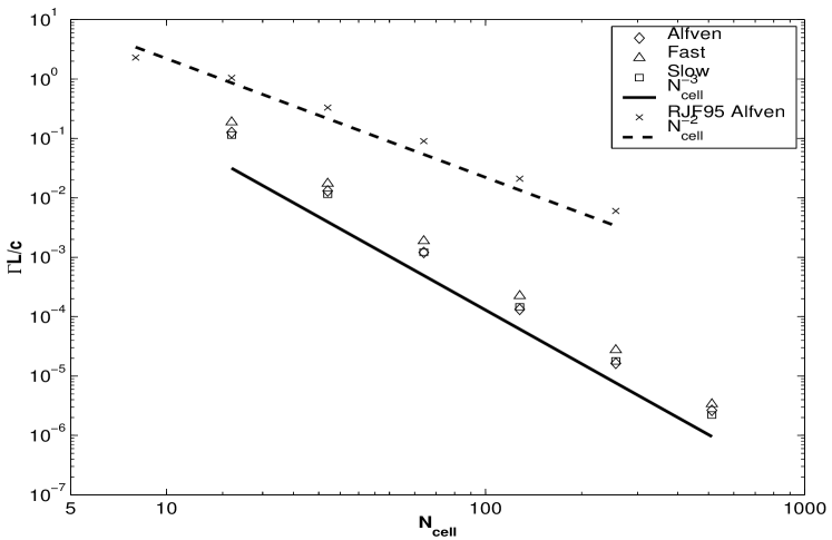
where $(\delta W)_{i,j}=W_{i,j}-W_{0}$ is the perturbation in the primitive variables. $l_{k}$ is the left-eigenvector associated with the mode in question, evaluated at $W_{0}$, the unperturbed state. Figure 2 shows the dependence of the decay rate on resolution for runs with number of cells per dimension $N=$16, 32, 64, 128, 256, and 512. Comparison with Figure 4 of RJF95 reveals a much smaller decay rate for our unsplit method. Furthermore, we find that the decay rate varies according to the power law $\Gamma\propto N^{-3}$, not $N^{-2}$. The former is consistent with second-order accuracy, since the truncation errors have the following form:

$$\tau=C_{2}(\Delta x)^{2}\frac{\partial^{3}U}{\partial x^{3}}+C_{3}(\Delta x)^{3}\frac{\partial^{4}U}{\partial x^{4}}+\mathcal{O}(\Delta x^{4}).$$ (53)

We see here that the second-order error term is proportional to $\frac{\partial^{3}U}{\partial x^{3}}$, which is dispersive in nature. The third-order term is the first error term that is dissipative. As a result, we expect the dissipation to decrease as $\Delta x^{3}$, or $N^{-3}$. We have no good explanation for the $\mathcal{O}(\Delta x^{2})$ decay law observed in RJF95, aside from the possible effects of artificial viscosity.

Figure 2: Normalized damping rate versus resolution for the decay of Alfvén, fast, and slow modes propagating at a 1:1 slope. The calculations were done at resolutions of $16\times 16$, $32\times 32$, etc. up to $512\times 512$.

4.3 MHD Shock Tube

The second test is the MHD shock tube problem from Ryu, Jones, and Frank [30]. The solution consists of two fast shocks, one slow shock, one slow rarefaction, and a contact discontinuity. We have run the problem in two orientations: (1) with the shock velocity aligned with the x-axis of the computational domain (referred to below as 1-D), and (2) with this velocity inclined at a 2:1 slope. The latter configuration follows the 2-D shock tube test case from T00. It was chosen in order to test the multidimensional behavior of the code, meanwhile ensuring there were no serendipitous cancellations of errors, as might be the case in a $45^{\circ}$ inclined case. In runs of a 1-D tube at $R_{512}$ (ie. 512 cells per linear dimension) on a domain of size $L=1$ to a time of $t=0.08$, we are able to reproduce the results given in Table VI of Dai & Woodward [11] (hereafter DW94) with errors of $\leq 0.12\%$. These results are independent of the type of filter used and whether an approximate projection was performed. Both the seven- and eight-wave codes give exactly the same result. When combined with an observed first-order convergence rate, they give us great confidence in the performance of both codes on 1-D shock tube problems.

The inclined version of this shock tube problem was run on grids of size $2N\times N$, with $N=64$, 128, and 256. Unlike in the aligned shock tube, in this case divergence cleaning is required. Since the natural boundary conditions for the problem would be tedious to implement in our multigrid solver, we chose instead to embed the physical domain within a larger one, four times its size. The data in the region outside of the original one is filled using the natural symmetry of the problem. The Poisson equation is then solved on this enlarged domain, using homogeneous Neumann boundary conditions. We have verified that the field in the original domain is clean to within the tolerances used previously.

We compared the results from the inclined shock tube with coarsened versions of a $R_{4096}$ 1-D shock tube results by first taking cuts of the data that included all cells lying along a line at 2:1 slope ($\alpha=26.57^{\circ}$). Then, all velocities and fields in the cut were rotated by $-\alpha$. A check using the initial conditions showed that such a cut of the inclined initial conditions matched perfectly with the 1-D shock tube ICs outside of the jump region. (In the jump region, the inclined ICs were slightly different due to the volume averaging performed in producing them. This leads the initial jump to be spread over two zones instead of one.) Note that we chose the grid spacing for the inclined runs to be a factor of $\sqrt{5}$ smaller than the 1-D grid spacing, so that the shock covers the same distance in physical space in a given time. The domain was therefore of length $L=1$ in the direction of shock propagation, and the final time $t=0.08$, in both the aligned and inclined shock runs.

Figure 3: MHD shock tube comparison by component. The 1-D shock tube (line) is used as a basis for comparison with 2-D shock tube runs with same effective resolution. The jumps in normal field $B_{n}$ are expected, and the size of the jumps is similar to that published in Tóth 2000.

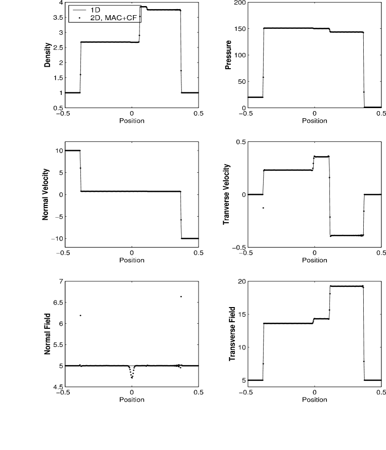
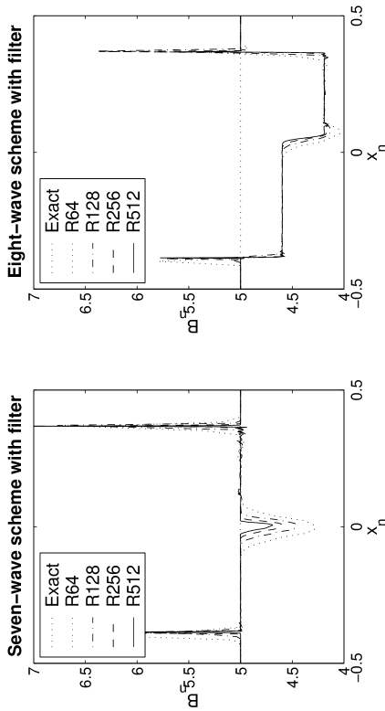
Figure 3 shows results for the inclined shock tube overlaid on the (coarsened) aligned result. They compare a $R_{256}$ 1-D run with a $N=256$ 2-D run that has equivalent effective grid spacing. The ideal MHD codes shown give fractional errors with an $L^{1}$ norm of 3% or less, averaged over all components. Errors in the normal component of the field are relatively large, however. As illustrated here and by Figure 11 in T00, shock-capturing codes generally produce unphysical variation in the normal component of the magnetic field inside the shock transition layer in non-grid-aligned shock tube problems such as this. More generally, such codes exhibit non-monotonic behavior inside the shock structure, so that Riemann invariants are not exactly preserved there [38]. Importantly, despite errors in $B_{n}$ inside the jump region, the jump relations are still satisfied outside of it. This is clearly illustrated in Figure 4, where we see the normal field for seven- and eight-wave schemes with filtering. Note in particular that while the eight-wave scheme converges to an answer, it does not give the correct shock structure.

Figure 4: Normal field results for MHD shock tube problem. Resolutions from $R_{64}$ to $R_{512}$ are shown. Note the incorrect shock structure in the eight-wave result.

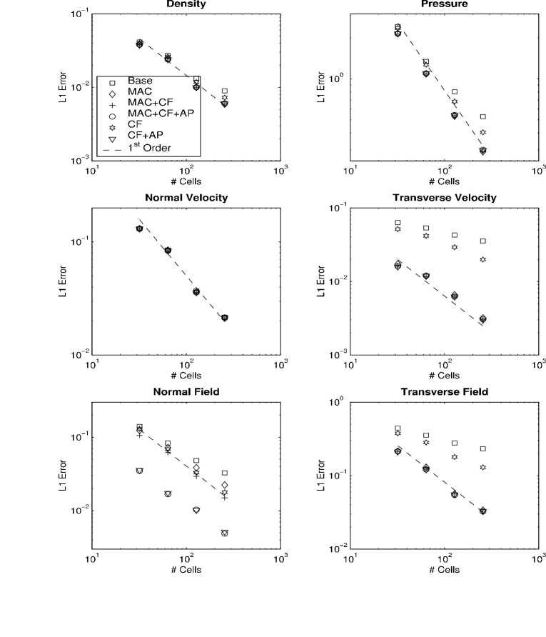
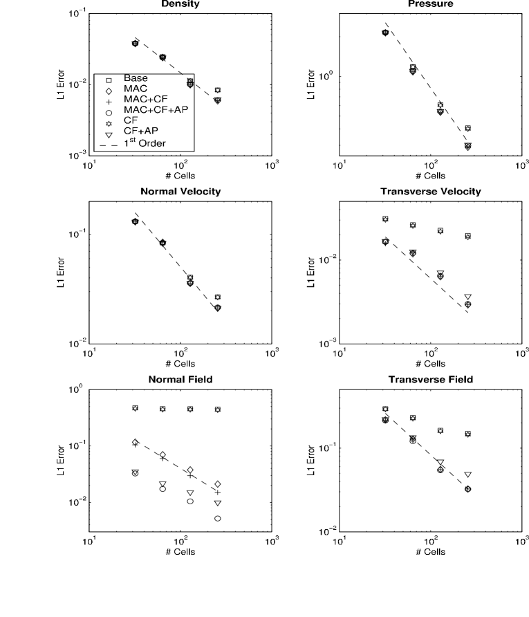
Figures 6 and 7 show plots of the $L^{1}$ norm of the error versus resolution for the 2-D shock tube runs. We first note that neither the seven- nor eight-wave base code converges at first order. This is most evident in the errors in the transverse velocity and transverse field. The same plots indicate filtering alone is not sufficient to produce reasonable convergence rates. A MAC projection step added to either scheme produces much improved results (label ’MAC’ in the figures), and the further addition of a filtering step gives first-order convergence in all components (label ’MAC+CF’). The use of an approximate projection (labels ’CF+AP’ and ’MAC+CF+AP’) produces decreased error in the normal field, indicating a more accurate solution at given resolution. However, no improvement in the convergence rates or errors in the other five components is observed. When averaged over all components, the decrease in error observed with an approximate projection is still noticeable, though less so than indicated by considering the normal field alone.

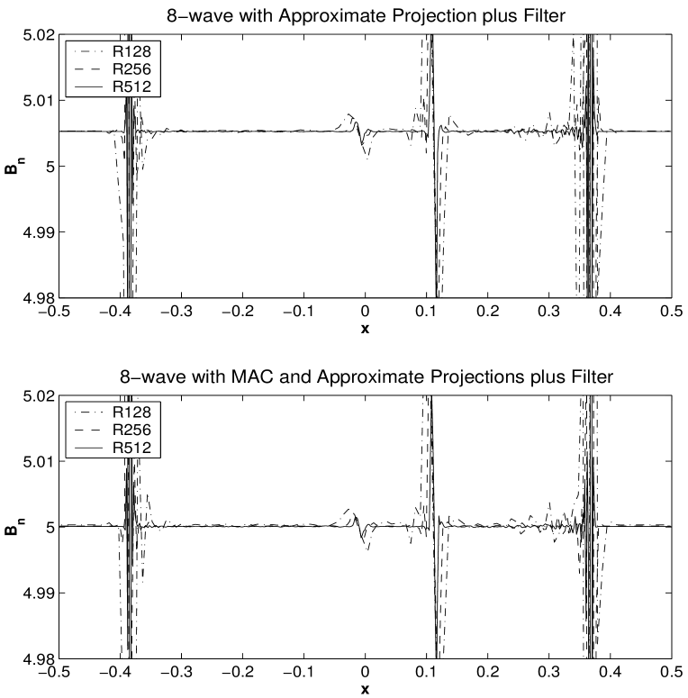
While the results for seven- and eight-wave codes with a MAC projection step are very similar, this picture changes somewhat when the MAC projection is replaced with an approximate projection (label ’CF+AP’). The seven-wave code gives identical results whether or not a MAC projection is used with the approximate projection and filter. The eight-wave code still exhibits smaller errors when an approximate projection is utilized. However, convergence of the errors for the eight-wave code with approximate projection alone stalls at higher resolution. The reason for this behavior becomes more clear upon closer inspection of the normal field, plotted in Figure 5. The normal field converges to an answer that is 0.1% above the expected value. This error, while masked by the larger errors at the jumps at lower resolution, becomes significant at higher resolution and consequently hampers convergence. This error is observed to grow steadily over time.

Figure 5: Normal component of the field for eight-wave codes with (bottom) and without (top) a MAC projection step. In these results for the inclined shock tube, a cut along the shock propagation direction is shown. The eight-wave code with the MAC projection converges to the correct answer, $B_{normal}=5$. Without the MAC projection, the code converges to an incorrect value for the normal field, about 0.1% higher than expected.

Figure 6: $L^{1}$ norm of error versus resolution (number of cells per dimension) for 2-D MHD shock tube run with variants of the seven-wave code. The dashed line is a fiducial showing first-order fall-off of errors. Note that some manner of projection step is required for first-order convergence.

Figure 7: $L^{1}$ norm of error versus resolution (number of cells per dimension) for 2-D MHD shock tube run with eight-wave codes. The dashed line is a fiducial showing first-order fall-off of errors.

4.4 Magnetized Flux Tube

This problem involves a high-field, low gas pressure region bounded on both sides by a high-gas pressure, zero-field region. The physical domain is of length $L_{x}=L_{y}=1$ on both sides. The base state has the entire 2-D domain in pressure balance. The boundaries between magnetized and unmagnetized regions are discontinuous and lie along $x=\pm 0.2$. In both regions, $\rho=1$, $\vec{u}=0$ and $B_{x}=B_{z}=0$ initially. In the magnetized region, $x\in[-0.2,0.2]$, $B_{y}=\sqrt{80\pi}$ and $P=1$. Outside of this, $B_{y}=0$ and $P=11$. To the background state is added a sinusoidal perturbation upon the x-velocity whose amplitude is $\delta_{\rm pert}=0.01$ times the Alfvén speed, and covers the entire domain:

$$\delta u=\delta_{\rm pert}c_{A}\sin\left(2\pi y\right)\;\;\textrm{and}\;\;\delta\vec{B}=\delta\rho=\delta P=\delta v=\delta w=0$$ (54)

The Alfvén speed in this case is $c_{A}=B_{0}/\sqrt{4\pi\rho}=\sqrt{20}$. The strong discontinuity in the field is expected to cause problems for algorithms that do not suppress non-solenoidal fields. In particular, at the stagnation points where the perturbation velocity is zero, truncation errors leading to non-solenoidal fields can build up and cause numerical schemes to go unstable. This is in fact what we find for base schemes run without a projection step. Non-solenoidal fields build up at these stagnation points, causing the production of spurious velocities and triggering numerical instabilities.

Figure 8: Grid-aligned (top) and inclined (bottom) flux tube initial conditions. Vectors indicate the perturbation velocity field; it is constant along lines parallel to the vectors. There are two regions: one magnetized, the other not. The entire domain is initially in total (magnetic plus thermal) pressure balance. The velocity perturbation at 1% of the Alfvén speed is applied to the entire domain, causing the tube and surrounding unmagnetized medium to oscillate.

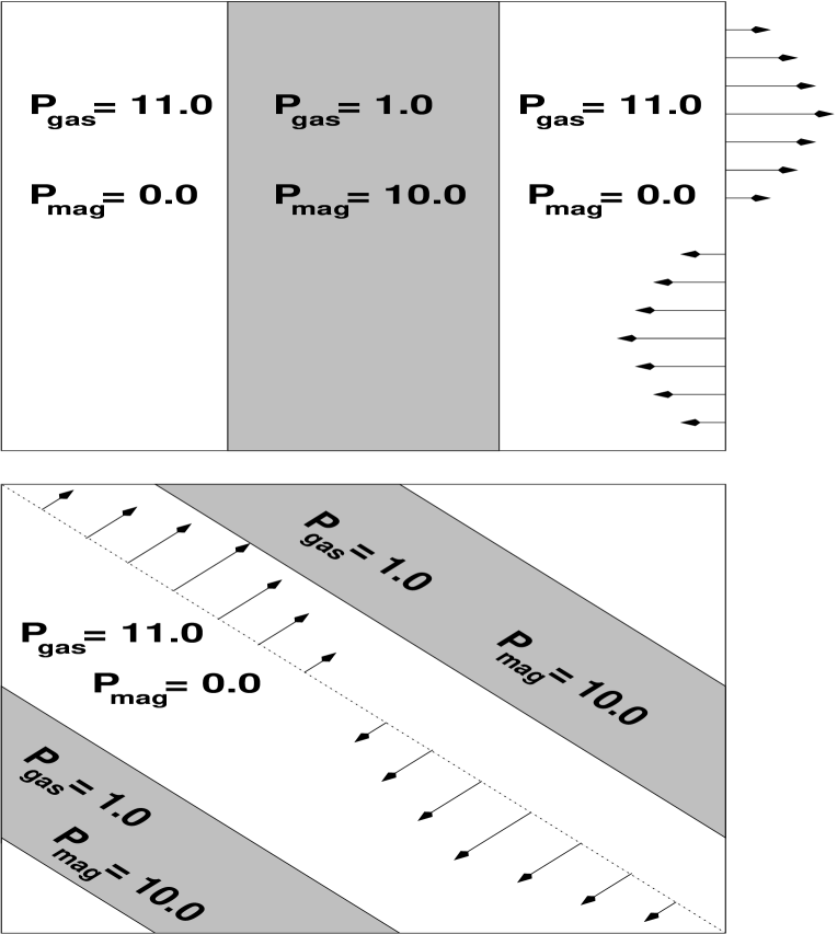
Figure 8 shows the initial conditions for the flux tube problem. The perturbation plucks the field. After an initial transient at start-up, the perturbation develops into a standing wave in the magnetized region. The unmagnetized region sloshes back and forth from one side of the flux tube to the other, owing to the periodic boundary conditions. We expect the initial velocity perturbation to cause standing Alfvénic waves in the magnetized region and, because of the slightly different oscillation frequencies of the two regions, compressive waves at the boundaries of the tube. The change in the internal energy tracks the compressive waves. The problem was run to a time $t=6.0$, corresponding to about 60 Alfvén crossings of the short dimension of the tube. This was enough time for the problem to exhibit stable periodic behavior and subsequently evolve for many periods of this oscillation.

Figure 9: Grid-aligned flux tube results at $R_{512}$. We use the $L^{1}$ norm of $\nabla\cdot\vec{B}$, plus total energies, to follow the evolution. Energies are normalized to their initial values. All quantities are plotted in units of the Alfvén crossing time, $t_{a}=1/c_{a}=0.2236$. Despite their different means of suppressing monopoles, the codes performed very similarly on this test.

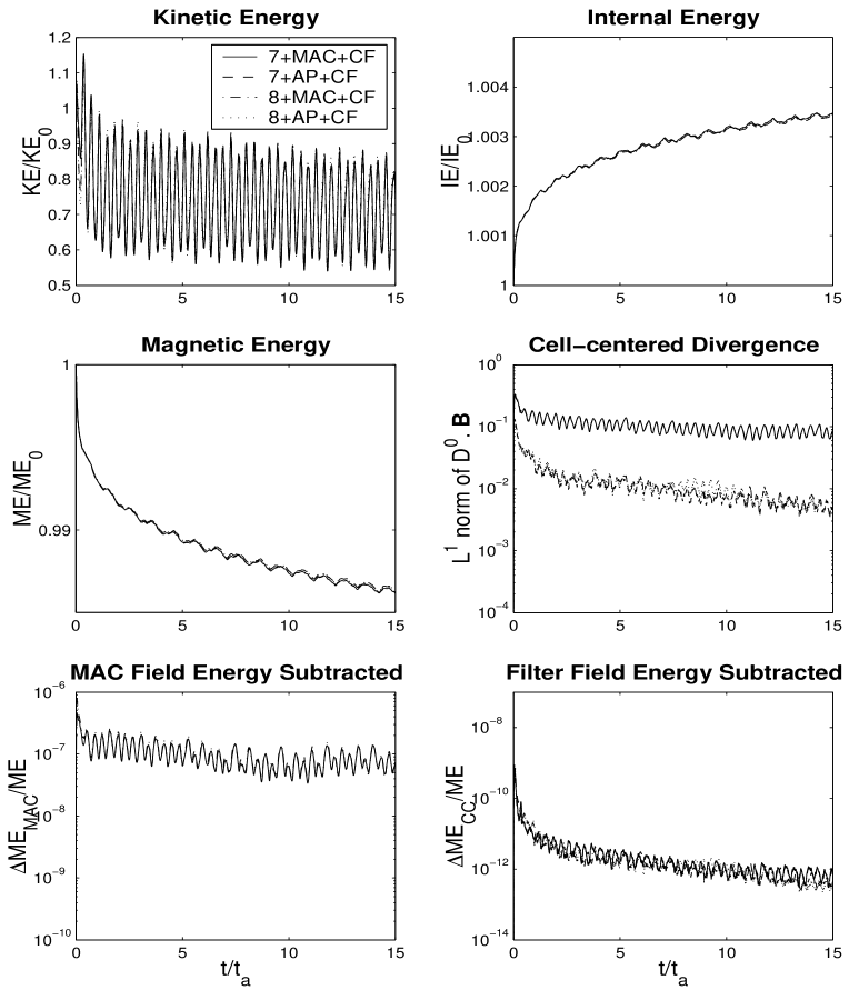
In this case we tested both seven- and eight-wave codes, but only with either a MAC projection and filter, or an approximate projection and filter. This is justified by the sub-par performance of the other variants on the inclined shock tube problem. These four versions of the code performed almost identically on this test, as evidenced by Figure 9. There, we plot global quantities such as kinetic and magnetic energy and $L^{1}$ norm of the monopole density. Note that the cell-centered divergence of the field is smaller for the approximate projection, though the dynamics remain the same.

4.5 Inclined Flux Tube

A second version of the flux tube problem, in which it is inclined at an angle of 45 degrees with respect to the original, is better at differentiating between the algorithms. It constitutes a strong test of the robustness and stability of the codes.

The size of the domain was $L_{x}=L_{y}=\sqrt{2}$, and both magnetized and unmagnetized regions have the same physical extent as in the aligned case. In both regions, we have $\rho=1$, $\vec{u}=0$ and $B_{z}=0$ initially. In the magnetized region, $B_{x}=-\sqrt{40\pi}$, $B_{y}=\sqrt{40\pi}$, and $P=1$. In the unmagnetized region, $P=11$ and $B_{x}=B_{y}=0$. The perturbation is again applied to the entire domain, and has strength $\delta_{\rm pert}=0.01$:

$$\delta u=\delta_{\rm pert}\frac{c_{A}}{\sqrt{2}}\sin\left(2\pi\frac{-x+y}{\sqrt{2}}\right)$$ (55)

$$\delta v=\delta_{\rm pert}\frac{c_{A}}{\sqrt{2}}\sin\left(2\pi\frac{-x+y}{\sqrt{2}}\right)$$ (56)

$$\delta\vec{B}=\delta\rho=\delta P=\delta w=0$$ (57)

One effect of rotating the flux tube is the addition of a numerical perturbation, or gridding effect. The volume-averaging required for producing the initial conditions creates a region of intermediate pressure and field between the fully magnetized and unmagnetized regions. The total pressure in this intermediate region was kept the same as elsewhere in the domain. The physical extent, and presumably physical effects, of this transition region become smaller as the resolution is increased. The second effect of our rotation is that the physical domain was somewhat larger. As mentioned above, this was done in order to keep the physical width of the magnetized and unmagnetized regions the same as for the aligned flux tube. The result is a factor of $\sqrt{2}$ mismatch between the grid spacing in the aligned and inclined flux tube runs.

We expect many qualitative similarities between the aligned and inclined flux tube results. The characteristics of the start-up transients are somewhat different, due in part to the gridding effects. The slightly different grid spacing also means that slightly higher resolution is required to obtain comparable results. Indeed, these tests were run at resolutions ranging by factors of two from $R_{128}$ to $R_{1024}$, a factor of two higher than for the aligned case.

Figure 10: Inclined flux tube results for one eight-wave (“8+MAC+CF”) and two seven-wave (“7+AP+CF” and “7+MAC+CF”) codes. The results for the different codes are also labeled with ’A’, ’B’, and ’C’, respectively. Since a MAC projection is not used in 7+AP+CF (’B’), no field energy is subtracted and it does not appear in the graph at lower-left. Note the relative size of increases in the kinetic energy of the codes, with smaller kinetic energies indicating stable oscillations. The eight-wave code with approximate projection and filter (“8+AP+CF”) was run on this problem as well, but became unstable.

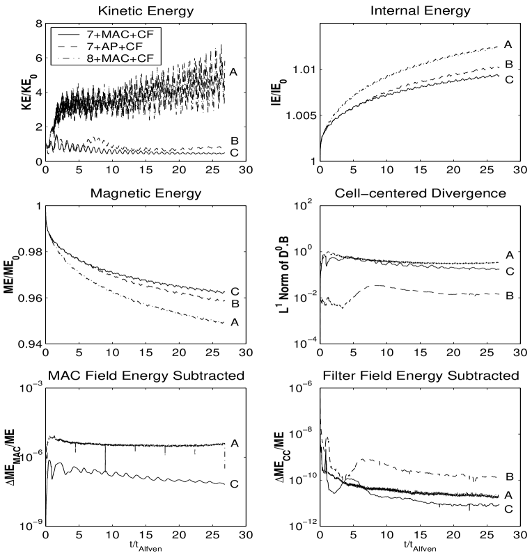
We again chose to run only those codes that showed close to first-order convergence for the inclined shock tube on this problem: seven- and eight-wave codes with either MAC projection and filter, or approximate projection and conservative filter. There was very little difference between the two seven-wave codes. The difference between seven- and eight-wave codes was more noticeable. The eight-wave codes both experienced large increases in kinetic energy, indicating that the magnetized tube was no longer in equilibrium. The size of this increase was largest ($\sim 10^{3}\rm{KE}_{\rm initial}$) for the eight-wave code with approximate projection, which also experienced substantial deviations from energy conservation. The size of these kinetic energy jumps decreased with resolution.

Figure 11: Inclined flux tube results for 256, 512, and 1024 cells in each direction. These results used the 7-wave MHD code with filtering and a coefficient of 0.1. The quantities shown are the same as in Figure 9.

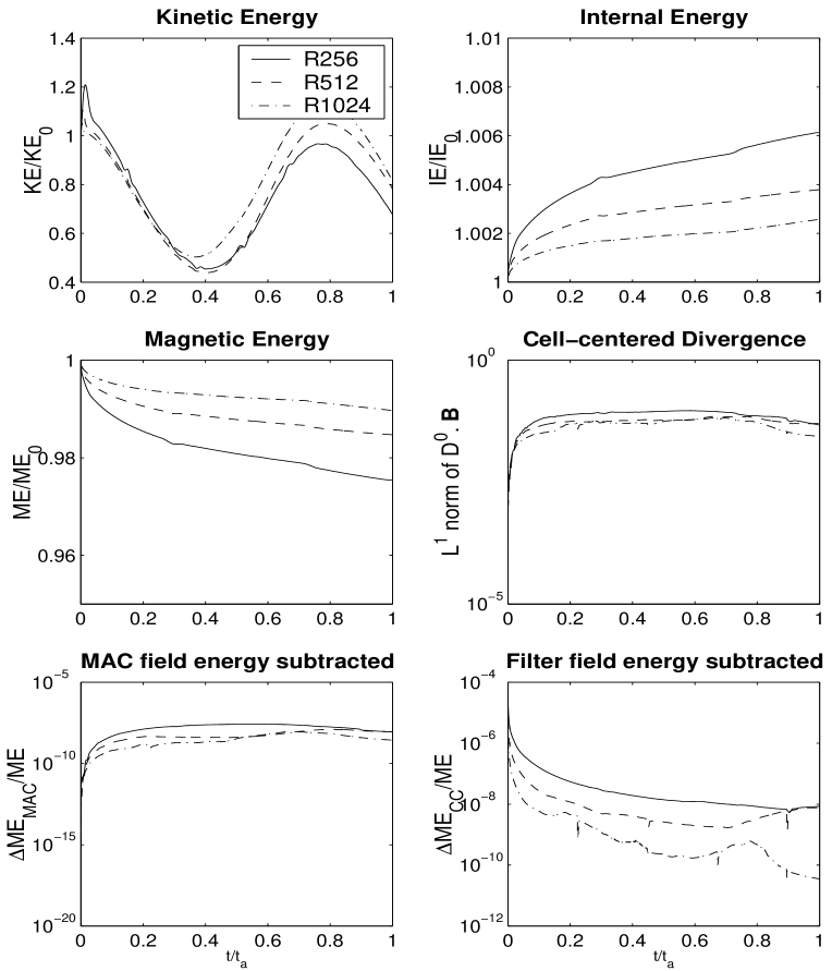
Figure 11 shows a resolution study of the inclined flux tube, with global quantities plotted out to $t=1$. (This is about 5 Alfvén crossing times; a shorter time was chosen in order to show more detail. All codes that were stable to this time were also stable out to $t=6$.) The plots include kinetic, internal, and magnetic energies, all scaled to their initial values. We also show the $L^{1}$ norm of cell-centered measure of the divergence, $D^{0}\cdot\vec{B}$, along with the magnetic energy change due to the MAC projection and filtering steps. First, note that the internal and magnetic energies appear to be converging, while convergence of the kinetic energy is not so clear. This result can be attributed to the large difference in the size of these quantities; the initial kinetic energy is $\sim 10^{5}$ times smaller than the initial internal energy, and $\sim 10^{4}$ times smaller than the initial magnetic energy. Thus, small errors in either of these quantities can appear as sizeable changes in the kinetic energy. We note in particular that increases in the kinetic energy seem to correlate with increases in the fraction of the magnetic energy subtracted in either the filter or the MAC projection.

The expected qualitative similarities between aligned and inclined flux tube results are present, such as oscillations in kinetic and magnetic energy of similar magnitudes. The size of the oscillations in the $L^{1}$ norm of $v_{t}$ and $v_{n}$ were also found to be very similar. However, substantial differences are also present. Comparing Figures 10 and 9, we note that the transient rise in kinetic energy early in the simulation begins later for the inclined tube than for the 1-D tube. In fact, the rise begins later and has smaller amplitude as resolution is increased, a fact that we attribute in part to the decrease in physical extent of the transition region.

Figure 12: Rotor problem results reproducing Figure 18 from T00. The plot has the same number of contours and these contours lie between the same limits. A slightly expanded domain was used ($x,y\in[-0.64,0.64]$) in order to preserve the same grid spacing.

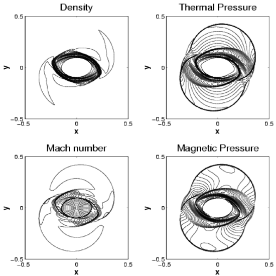
As a final test of the nonlinear behavior of the code, we reproduce the first MHD rotor problem outlined in T00, earlier performed by Balsara and Spicer [5]. This problem constitutes a central, high-density ($\rho=10.0$) region surrounded by a low-density medium. The central region is given a constant angular velocity. The entire domain is threaded by an initially constant field, $\vec{B}=5.0\hat{e}_{x}$. The rotation winds the magnetic field, sending Alfvén waves propagating into the surrounding medium.

This test was run using both seven-wave codes (MAC+CF and AP+CF) and one eight-wave variant (MAC+CF). We see no negative pressures in any of the code variants, and obtain first-order convergence (errors decreasing as the grid spacing to the 0.95 power, as averaged over all variables) using the seven-wave codes, and the eight-wave code with a MAC projection. A reproduction of Figure 18 from T00 is given in Figure 12. Note the steeper gradient in Mach number in comparison to the T00 result; we do not see the peaks therein attributed to pressure undershoots.

5 Conclusions

We have presented an unsplit method for ideal MHD which, when combined with projection and filtering steps, shows no effects of non-solenoidal fields, while retaining the co-location of all physical quantites at cell-centers. The latter point is important because such a uniform centering makes it easier to extend the scheme to adaptive meshes, and has the advantage of using a well-understood Godunov method for time integration. These are in contrast to the Constrained Transport (CT) approach, where staggered grids add additional software complexity. Furthermore, it is not obvious how to discretize diffusion operators to include non-ideal MHD effects on staggered grids. Lastly, we add that the effective advection scheme for the magnetic field components is not of the standard type, and it is unclear what its properties are in the presence of under-resolved gradients.

The complexity and cost of the scheme relative to others is an important consideration. Our scheme requires three characteristic analysis steps plus twelve Riemann solution steps in 3-D. This is comparable to the six characteristic analysis and six Riemann solution steps required in a two-step Runge-Kutta scheme. The computational cost of projection is not insignificant, and adds additional software complexity. On a single grid and a single processor, the cost of the projection when computed using FFTs is a small fraction of the overall cost of the computation (less than 200 floating-point operations per cell in 3D). Current research on analysis-based solvers for Poisson’s equation [21, 4] have the potential to make the cost of this remain less than that of the hyperbolic calculation, on both adaptive grids and on parallel processors.

The Hodge projection of fields either at cell-edges (MAC projection) or cell-centers (in our case via an approximate projection) was found to be essential to accuracy and stability. The MAC projection was essential for accuracy of the eight-wave code in the presence of discontinuities. The seven-wave code results on the inclined shock tube were less sensitive to the type of projection used. The inclined flux tube results painted essentially the same picture, though the seven-wave MAC projected result was somewhat more robust.

Use of a filter alone on linear problems reduces computational cost and does not affect accuracy. We find that both filter and projection are required on strongly nonlinear problems such as the inclined flux tube. Also essential to the accuracy of the scheme are the modifications suggested by Stone – linear waves not propagating along coordinate-axis directions are not second-order accurate without it.

We found that in determining the accuracy of our code, both measuring the rate of convergence on nonlinear problems and comparing absolute magnitude of the error were required. Significant differences were found between the convergence rates even of individual primitive variables. These data can be crucial in choosing between different algorithmic variants of a base code. We encourage future authors to incorporate convergence testing, taking care to calculate errors in each variable separately, of simple nonlinear problems such as the shock tubes run here into their test suites.

Overall the ideal MHD code with a projection, either MAC or approximate, and a filter performed best on the suite of tests presented. Filtering of the magnetic field was important to code stability in the nonlinear problems, and accuracy in the deficient wave problems.

The magnetized, perturbed flux tube constitutes a strong test of the stability of our schemes. The combination of a stationary discontinuity, low ratio of thermal to magnetic pressure (beta), and imposed perturbation caused significant problems for the base unsplit code without projection or filter. With a suitably chosen value of the filtering coefficient, the filter helped stability and worked to decrease the magnitude of a centered-difference measure of the divergence of the field.

6 Acknowledgements

The authors would like to thank Jim Stone for pointing out the missing multidimensional MHD terms.

The research of Robert K. Crockett was supported in part by A Division at Lawrence Livermore National Laboratory.

The research of Christopher F. McKee was supported in part by NSF grant AST-0098365.

Work at the Lawrence Berkeley National Laboratory is sponsored by the US Department of Energy Applied Mathematical Sciences program under contract DE-AC03-76SF00098 and by the NASA Earth and Space Sciences Computational Technologies Program under interagency agreement number S-44830-X.

The research of Richard I. Klein was supported in part by a NASA ATP grant NAG5-12042. Both Richard I. Klein and Robert T. Fisher are supported under the auspices of the US Department of Energy at the Lawrence Livermore National Laboratory under contract W-7405-ENG-48.

Appendix A Appendix A: Divergence Constraints, Modified Equation Analysis, and Eigenvector Deficiencies

In this section, we will present a heuristic analysis of the effect of numerical errors in the divergence-free constraint on the stability of finite-difference methods for the ideal MHD equations. Our starting point will be the modified equation approach to analyzing the effect of truncation error on solution error. For any finite difference method, the modified equation is given by the original system of PDEs, with forcing terms given by the truncation error. In the present setting, the modified equation takes the following form:

$$\partial_{t}U^{Mod}+\nabla\cdot\vec{F}(U^{Mod})=\tau_{U}(U^{Mod})$$ (58)

$$\nabla\cdot\vec{B}^{Mod}=\tau_{D}(U^{Mod}).$$ (59)

Here $\tau_{U}$ is the usual truncation error for the numerical method obtained from applying the difference operator to a solution to the differential equation evaluated on the grid. The equation for the evolution of $\tau_{D}$ is obtained by taking the divergence of the modified equation for the evolution of $U^{Mod}$,

$$\partial_{t}\tau_{D}=\nabla\cdot\tau_{B}.$$ (60)

The truncation error forcing terms mimic the effect of numerical error on the computed solution. Specifically, we expect $U^{Mod}$, the solution to the modified equation, to satisfy $||U^{\Delta x}-U^{Mod}||=\mathcal{O}(\Delta x^{p+1})$, where $U^{\Delta x}$, the solution obtained from the $p^{\rm th}$-order scheme on a grid with spacing $\Delta x$, satisfies $||U^{\Delta x}-U||=\mathcal{O}(\Delta x^{p})$.

In particular, for MHD, the effect of numerical error can be understood in terms of the truncation-error forcing in the modified equation causing the solution to violate the divergence-free constraint. Without that constraint being satisfied, the remaining ideal MHD equations can exhibit eigenvector deficiencies in the linearized-coefficient matrix $\mathbf{A}$, leading to anomalous loss of regularity and ill-posedness. In the numerical simulation, this translates into loss of accuracy and possibly instability of the underlying difference method.

To see this, we consider the case of a small-amplitude wave corresponding to one of the eigenmodes of $\mathbf{A}$ (see Equation 8):

$$W(\vec{x},\,t)=W_{0}+\alpha(x-\lambda_{k}t)r_{k}$$ (61)

$$\mathbf{A}_{0}r_{k}=\lambda_{k}r_{k}\;\;r_{k}=(\tilde{r}_{k},\,0)^{T}.$$ (62)

Then $W(\vec{x},\,t)$ satisfies the MHD equations up to terms of $\mathcal{O}(\alpha^{2})$.

Without loss of generality, we take the direction of propagation to be in the x-direction in 3-D. However, we allow our computational spatial grid to have an arbitrary orientation in space. In that case, the modified equation corresponding to our numerical solution to the PDE in primitive variables $W$ is given by (see Equation 7)

$$\partial_{t}W^{Mod}+\mathbf{A}_{0}\partial_{x}W^{Mod}=\tau_{W}$$ (63)

$$W^{Mod}=(\tilde{W}^{Mod},\,B_{x}^{Mod}).$$ (64)

If we define the new variable $\alpha^{Mod}=l_{k}\cdot(\tilde{W}^{Mod}-\tilde{W}_{0})$, the modified equation dynamics can be reduced to the following system of two equations:

$$\partial_{t}\alpha^{Mod}+\lambda_{k}\partial_{x}\alpha^{Mod}+(l_{k}\cdot a_{B})\partial_{x}B_{x}^{Mod}=l_{k}\cdot\tilde{\tau}$$ (65)

$$\partial_{t}B_{x}^{Mod}=\tau_{B}$$ (66)

In the system here, if one of the computational spatial grid coordinate axes is aligned with $\hat{x}$, $\tau_{B}\equiv 0$. However, if the direction of propagation is not aligned with one of the computational coordinates, then in general $\tau_{B}\neq 0$. If $l_{k}\cdot a_{B}\neq 0$ and $\lambda=0$, then the left-hand side of 65-66 is an example of a first-order system with an eigenvector deficiency. Such systems have an obvious loss of spatial regularity: $\alpha^{Mod}$ grows like the derivative of $\tau_{B}$. This is in contrast to the behavior of well-posed hyperbolic systems, in which the solution has the same spatial regularity as the forcing. In other words, since regularity implies that there are as many derivatives in the solution as in the forcing term, discontinuous forcing of a hyperbolic system leaves the problem ill-posed. Discontinuity in $\tau_{B}$ implies that $\alpha^{Mod}$ can grow without bound, owing to its dependence on the derivative of $\tau_{B}$.

In terms of a numerical method, we expect that the presence of such terms would lead to either an anomalous loss of accuracy or numerical instability. In the latter case, the forcing of $\alpha^{Mod}$ in 65 takes the form of a finite difference operator applied to $B_{x}^{Mod}$, whose spatial variation is due entirely to $\tau_{B}$. If $\tau_{B}$ fails to be smooth, either because of lack of smoothness in the initial data or in the finite difference formulae (eg. limiters), such lack of smoothness is immediately amplified.

This discussion also provides an explanation for the behavior of the method described here. The use of the MAC projection and the filter does not eliminate the truncation error terms that lead to the eigenvector deficiency, but regularizes it by smoothing. For example, the application of the filter in the plane-wave example corresponded to adding a diffusion term to the equation for $B_{x}^{Mod}$,

$$\partial_{t}B_{x}^{Mod}=\tau_{B}+\eta\partial_{x}^{2}B_{x}^{Mod},$$ (67)

with $\eta=\mathcal{O}(\Delta x)$. The use of the filter alone is sufficient to stabilize the small-amplitude plane wave solution in Section 4.1, and in that case leads to a second-order accurate result. The MAC projection performs a more drastic smoothing, but only on the intermediate form of $B_{x}^{Mod}$ used to compute $\partial_{x}B_{x}^{Mod}$ in equation 65.

References

- [1] A. S. Almgren, J. B. Bell, and W. Y. Crutchfield, Approximate Projection Methods: Part I. Inviscid Analysis, SIAM J. Sci. Comput. 22(4) (2000) 1139-59.
- [2] A. S. Almgren, J. B. Bell, and W. Szymczak, A numerical Method for the Incompressible Navier-Stokes Equations Based on an Approximate Projection, SIAM J. Sci. Comput. 17 (1996) 358.
- [3] D. S. Balsara, Total Variation Diminishing Scheme for Adiabatic and Isothermal Magnetohydrodynamics, Astrophys. J. Suppl. 116 (1998) 133.
- [4] G. Balls and P. Colella, A Finite Difference Domain Decomposition Method Using Local Corrections for the Solution of Poisson’s Equation, J. Comput. Phys. 180 (2002) 25-53.
- [5] D. S. Balsara and D.S. Spicer, A Staggered Mesh Algorithm Using High Order Godunov Fluxes to Ensure Solenoidal Magnetic Fields in Magnetohydrodynamic Simulations, J. Comput. Phys. 149 (1999) 270.
- [6] J. B. Bell, P. Colella, and L. H. Howell, An Efficient Second-Order Projection Method for Viscous Incompressible Flow, in AIAA 10th Computational Fluid Dynamics Conference Proceedings, June 1991, 360.
- [7] J. B. Bell, P. Colella, and J. A. Trangenstein, Higher Order Godunov Methods for General Systems of Conservation Laws, J. Comput. Phys. 82 (1989) 362.
- [8] J. U. Brackbill and D. C. Barnes, The Effect of Nonzero div(B) on the Numerical Solution of the Magnetohydrodynamic Equations, J. Comp. Phys. 35 (1980) 426.
- [9] M. Brio and C.C. Wu. An Upwind Differencing Scheme for the Equations of Ideal Magnetohydrodynamics. J. Comp. Phys. 75 (1988), 400.
- [10] P. Colella, Multidimensional Upwind Methods for Hyperbolic Conservation Laws, J. Comput. Phys. 87 (1990) 171.
- [11] W. Dai and P. R. Woodward, An Approximate Riemann Solver for Ideal Magnetohydrodynamics, J. Comput. Phys. 111 (1994) 354.
- [12] W. Dai and P. R. Woodward, Extension of the Piecewise Parabolic Method to Multidimensional Ideal Magnetohydrodynamics. J. Comput. Phys. 115 (1994), 485.
- [13] W. Dai and P. R. Woodward, A Simple Finite Difference Scheme for Multidimensional Magnetohydrodynamical Equations, J. Comput. Phys. 142 (1998), 331.
- [14] A. Dedner, F. Kemm, D. Kröner, C.-D. Munz, T. Schnitzer, and M. Wesenberg, Hyperbolic Divergence Cleaning for the MHD Equations, J. Comp. Phys 175 (2002) 645.
- [15] C. R. Evans and J. F. Hawley, Simulation of Magnetohydrodynamic Flows: A Constrained Transport Method, Astrophys. J. 332 (1988) 659.
- [16] S. A. Falle, Rarefaction Shocks, Shock Errors, and Low Order of Accuracy in ZEUS, Astrophys. J. 577 (2002), L123.
- [17] S. K. Godunov, The Symmetric Form of Magnetohydrodynamics Equation, Numer. Methods Mech. Contin. Media 1 (1972) 26.
- [18] T. I. Gombosi, K. G. Powell, and D. L. DeZeeuw, Axisymmetric Modeling of Cometary Mass Loading of an Adaptively Refined Grid: MHD Results, J. Geophys. Res. 99 (1994) 21, 525.
- [19] F. Harlow and J. Welch, Numerical Calculation of Time-Dependent Viscous Incompressible Flow of Fluids with Free Surfaces, Physics of Fluids 8 (1965) 2182.
- [20] L. H. Howell and J. B. Bell, An Adaptive-Mesh Projection Method for Viscous Incompressible Flow, SIAM J. Sci. Comp. 18 (1997), 996-1013.
- [21] J. F. Huang and L. Greengard, A Fast Direct Solver for Elliptic Partial Differential Equations on Adaptively Refined Meshes, SIAM Journal on Scientific Computing. 21(4) (2000) 1551-1566.
- [22] M. F. Lai, A Projection Method for Reacting Flow in the Zero Mach Number Limit, Ph.D. Thesis, UC Berkeley 1993.
- [23] Londrillo, P. and Del Zanna, L., High-Order Upwind Schemes for Multidimensional Magnetohydrodynamics, Astrophys. J. 530 (2000), 508.
- [24] B. Marder, A Method for Incorporating Gauss’ Law into Electromagnetic PIC Codes, J. Comput. Phys. 68 (1987) 48.
- [25] D. F. Martin and P. Colella, A Cell-centered Adaptive Projection Method for the Incompressible Euler equations, J. Comput. Phys. 163(2) (2000), 271-312.
- [26] Miller, G. H. and Colella, P. A High-Order Eulerian Godunov Method for Elastic-Plastic Flow in Solids, J. Comput. Phys. 167 (2001) 131.
- [27] K. G. Powell, P. L. Roe, T. J. Linde, T. I. Gombosi, D. L. De Zeeuw, A Solution-Adaptive Upwind Scheme for Ideal Magnetohydrodynamics, J. Comput. Phys. 154 (1999), 284.
- [28] W. J. Rider, Filtering Non-solenoidal Modes in Numerical Solutions of Incompressible Flows. IJNMF 28, 789.
- [29] P. L. Roe and D. S. Balsara, Notes on the Eigensystem of MHD, SIAM J. Appl. Math. 56 (1996) 57.
- [30] D. Ryu, T. W. Jones, and A. Frank, Numerical Magnetohydrodynamics in Astrophysics: Algorithm and Tests for Multidimensional Flow. Astrophys. J 452 (1995) 785.
- [31] D. Ryu, F. Miniati, T. W. Jones, and A. Frank. A Divergence-free Upwind Code for Multidimensional Magnetohydrodynamic Flows, Astrophys. J. 509 (1998) 244.
- [32] F. Shu. The Physics of Astrophysics: Gas Dynamics. University Science Books (1992).
- [33] J. M. Stone and M. L. Norman, ZEUS2D: A Radiation Magnetohydrodynamics Code for Astrophysical Flows in Two Space Dimensions. II The Magnetohydrodynamic Algorithms and Tests, Astrophys. J. Suppl. 80 (1992) 791.
- [34] T. A. Gardiner and J. Stone, An Unsplit Godunov method for Ideal MHD via Constrained Transport, preprint, April 2004, submitted to J. Comput. Phys.
- [35] E.F. Toro, Riemann Solvers and Numerical Methods for Fluid Dynamics : A Practical Introduction. Springer-Verlag (1999).
- [36] G. Tóth, The div(B) Constraint in Shock-Capturing Magnetohydrodynamics Codes. J. Comp. Phys. 161 (2000) 605.
- [37] G. Tóth, Conservative and Orthogonal Discretization of the Lorentz Force. J. Comp. Phys. 182 (2002) 346.
- [38] P. R. Woodward, Piecewise Parabolic Methods for Astrophysical Fluid Dynamics, in Astrophysical Radiation Hydrodynamics, K.-H. Winkler and M. Norman, eds. Reidel (1986) 245.
- [39] A. L. Zachary, A. Malagoli, and P. Colella, A Higher-order Godunov Method for Multidimensional Ideal Magnetohydrodynamics, SIAM J. Sci. Comput. 15 (1994) 263.
- [40] A. L. Zachary and P. Colella, A Higher-order Godunov Method for the Equations of Ideal Magnetohydrodynamics, J. Comput. Phys. 99 (1992) 341.