Cluster Masses Accounting for Structure along the Line of Sight

Abstract

Weak gravitational lensing of background galaxies by foreground clusters offers an excellent opportunity to measure cluster masses directly without using gas as a probe. One source of noise which seems difficult to avoid is large scale structure along the line of sight. Here I show that, by using standard map-making techniques, one can minimize the deleterious effects of this noise. The resulting uncertainties on cluster masses are significantly smaller than when large scale structure is not properly accounted for, although still larger than if it was absent altogether.

Introduction. Clusters of galaxies are powerful cosmological probes cluster . In particular, the number density of clusters as a function of mass and redshift depends sensitively on the cosmological growth function which in turn depends on the matter density and properties of the dark energy wang . Indeed, it is conceivable that we will learn as much about dark energy from clusters as from supernovae haiman .

While redshifts of clusters are relatively easy to obtain, cluster masses are much harder to pin down. A cluster mass can be estimated from optical richness or from its temperature, measured either in the X-ray or with radio observations of the Sunyaev-Zel’dovich distortion of the cosmic microwave background. However, the scatter around any of these indicators is large scatter and depends on complicated physics, such as radiative transfer, star and galaxy formation, cooling, accretion, and feedback mechanisms. In principle, gravitational lensing bartel allows for a more direct mass determination, since the distortions of background galaxies are sensitive only to the mass along the line of sight, not to the gas. In practice, there are many hurdles to overcome, most of which involve the observations themselves.

There is one systematic that affects lensing determinations of clusters that cannot be cured with better instruments or seeing. Large scale structure along the line of sight can be mistaken as being part of the cluster los . As Hoekstra hoekstra has shown, the uncertainties caused by this noise can significantly impair our ability to estimate cluster masses. Since cluster abundances depend sensitively on their masses, this uncertainty clouds the possiblity of learning about dark energy from clusters.

Here I show that one can partially offset the deleterious effects of large scale structure by accounting for it in cluster mass estimates. To demonstrate how this works, I will focus on a single cluster at redshift $0.3$ with a Navarro, Frenk, and White (NFW) profile nfw . The mass enclosed within a radius within which the average density is $200$ times as large as the critical density, $M_{200}$, will be set to $1.4\times 10^{15}M_{\odot}$ and the concentration $c$ to $4.64$. I will assume we have ellipticities for thirty background galaxies per square arcminute, all at redshift one. These parameters will allow us to compare with the results of Ref. hoekstra .

Effects of Large scale structure. To get a feel for some numbers, the shear due to this cluster has magnitude equal to $0.02$ at an angular distance $10^{\prime}$ away from the center. In a one square arcminute pixel with thirty background galaxies, the rms noise due to the galaxy uncertainties is $0.25/\sqrt{30}=0.046$, significantly larger than the signal. The rms noise due to large scale structure is of order $0.02$ for a standard $\Lambda$CDM model. Adding the two sources of noise in quadrature leads to a ten percent increase in the noise due to large scale structure. Hoekstra hoekstra however showed that the situation is not that simple. Since the signal to noise in each pixel is small, it is necessary to average over many pixels with the same signal, in this radially symmetric case, over azimuthal angle at fixed radius.

If we average over all pixels in an annulus of width $1^{\prime}$ at radius of $10^{\prime}$, then the shape noise gets reduced by a factor of $N_{p}^{-1/2}$ where $N_{p}$ is the number of pixels, approximately equal to $20\pi$. The shape noise contribution to this angular average then should be of order $0.046/(20\pi)^{1/2}\simeq 0.006$, significantly smaller than the signal. If the noise due to large scale structure was completely independent from one pixel to the next, then it too would be reduced by the same factor, and would have an rms amplitude of $0.0025$. Figure 1 shows that shape noise does behave as expected, but the noise due to large scale structure is larger than anticipated by more than a factor of two. Apparently, large scale structure produces a signal (noise) which is correlated over many pixels. The number of independent pixels then is much smaller than $20\pi$, and the contamination of the cluster signal from large scale structure is much more severe than one might naively estimate. As shown in Figure 1, the situation rapidly gets worse at larger angles, so Hoekstra argued that measurements beyond $15^{\prime}$ were useless for determining the cluster mass profile: the noise from large scale structure overwhlems the useful information in such measurements.

Figure 1: Azimuthally averaged tangential shear gamt . Also shown is the rms noise due to uncertainty in background galaxy shapes and due to large scale structure.

The above hand-waving argument suggests a possible solution. Since the large scale structure signal is correlated over $\sim 4^{\prime}$, why not make use of this correlation in the radial direction as well? That is, when averaging over the azimuthal shear, one implicitly discards all information about the combined radial/azimuthal structure of the shear. A circular blob of shear with diameter $4^{\prime}$ due to large scale structure might be easily detected before the angular averaging and then subtracted off. If we first average over angles, we lose much of our power to identify and account for the shear due to large scale structure.

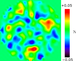
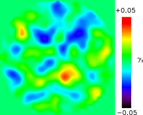
Figure 2: Top panel: Tangential shear $\gamma_{t}$ due to a realization of shape noise; Middle panel: $\gamma_{t}$ from large scale structure in a single realization. The noise emanating from large scale structure is much more coherent than that due to the uncertainty in galaxy shapes. Note especially the swath of negative $\gamma_{t}$ in the bottom panel extending from lower left to upper right. Bottom Panel: The same two realizations smoothed over azimuthal angle. There is no longer any clear distinction between the two sources of noise.

This is illustrated in Fig. 2, where a realization of each source of noise is shown in the top two panels. The noise from large scale structure is manifestly more coherent, extending over larger scales than is the shape noise. Just as clearly, this distinction disappears (bottom panel) if one averages over azimuthal angle.

In order to retain the information necessary to distinguish large scale structure shear from cluster shear, we need to start from the full shear field, $\gamma_{i}(\vec{\theta}_{a})$, where $i=1,2$ labels the two components of the symmetric, traceless shear tensor. Assuming that the shear induced by large scale structure is Gaussian, the likelihood of obtaining the data is

$${\cal L}={[2\pi]^{-N_{p}}\over\det(N)^{1/2}}\exp\left\{-\frac{1}{2}\big{(}\gamma_{\alpha}-\gamma_{\alpha}^{\rm cl}\big{)}[N^{-1}]_{\alpha\beta}\big{(}\gamma_{\beta}-\gamma_{\beta}^{\rm cl}\big{)}\right\}$$ (1)

where the index $\alpha$ includes both pixel position ($a$) and shear component ($i$) so ranges from 1 to $2N_{p}$, with $N_{p}$ now the total number of pixels for which we have ellipticities. The noise matrix $N$ is the sum of the covariance due to shape noise and to large scale structure,

$$N\equiv C^{\rm shape}+C^{\rm lss}.$$ (2)

From this starting point, there are a number of directions one can take. Here I pursue two: (i) using the likelihood function and the Fisher matrix derived from it to project uncertainties on the two parameters characterizing the NFW profile and (ii) compressing the information in the likelihood function into a mass estimator which is optimal in the sense that it retains all the relevant information. In both cases, we can compare the results with what one would obtain without accounting for large scale structure.

Parametric Fitting.

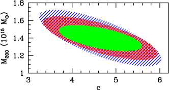
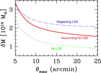
Figure 3: Top panel: Projected 1-sigma errors on $M_{200}$ and concentration from ellipticities within $20^{\prime}$ of the cluster assuming $30$ background galaxies per square arcminute, all at redshift 1. Inner ellipse assumes there is no contribution from large scale structure. Outer ellipse shows the increase in errors once large scale structure is included. Middle ellipse also includes large scale structure, but here the parameters are determined directly from the likelihood function, instead of from $\langle\gamma_{t}\rangle$. Bottom panel: Errors on the mass of the cluster as a function of the maximum angle out to which ellipticities of background galaxies are measured.

Let’s assume that the cluster we are studying has an NFW profile and ask how well we can determine the parameters characterizing this profile. The Fisher matrix,

$$F_{ij}\equiv-{\partial^{2}{\cal L}\over\partial p_{i}\partial p_{j}}={\partial\gamma^{\rm cl}_{\alpha}\over\partial p_{i}}[N^{-1}]_{\alpha\beta}{\partial\gamma^{\rm cl}_{\beta}\over\partial p_{j}},$$ (3)

quantifies the errors on these parameters $p_{1}(M_{200})$ and $p_{2}(c)$ from a lensing survey. We will consider the errors on $M_{200}$ and $c$ in three cases: (i) no large scale structure, $N=C^{\rm shape}$; (ii) including and accounting for large scale structure $N=C^{\rm shape}+C^{\rm lss}$; and (iii) large scale structure present, but parameters determined from the azimuthally averages tangential sheargamt , $\langle\gamma_{t}\rangle$. In this last case, the data points $\gamma_{\alpha}$ in equation [3] are replaced by $\langle\gamma_{t}\rangle$ in different radial bins and the noise matrix $N_{\langle\gamma_{t}\rangle}$ consists of the shape noise per pixel reduced by the number of pixels in the azimuthal average and the azimuthally averaged large scale structure covariance matrix. Incidentally, if no large scale structure is present (i), then using all the pixels is not necessary: $\langle\gamma_{t}\rangle$ maintains all the relevant information.

The top panel of Figure 3 shows the projected errors from a survey which measures background galaxies within $20^{\prime}$ of the cluster center. The difference between the inner and outer ellipse reinforces the point emphasized by Hoekstra hoekstra , that the noise due to large scale structure degrades the parameter determination by a factor of order two if not properly accounted for. The middle ellipse shows though that the situation is not quite this dire. If one works from the likelihood function directly and does not azimuthally average, the effects of large scale structure can be minimized.

The bottom panel of Fig. 3 shows the error on $M_{200}$ (after marginalizing over the concentration) in these three cases as a function of the maximum distance out to which data is available. Here we can see that the optimal estimator (i.e. not azimuthally averaging) reduces the deleterious effects of large scale structure by roughly $50\%$ at least on large scales. This realization has practical implications: is it worthwhile taking data far from the cluster center or does the noise due to large scale structure make such data irrelevant when it comes to determining the cluster mass? Figure 3 shows that going out to $25^{\prime}$ leads to a fifteen percent smaller error on $M_{200}$ as compared with $\theta_{\rm max}=15^{\prime}$. While this is not quite as large as the $18\%$ gain if there was no large scale structure, it is much larger than five percent gain if large scale structure is not accounted for.

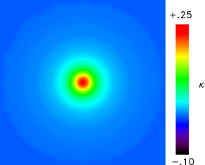
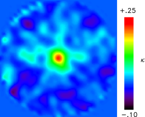
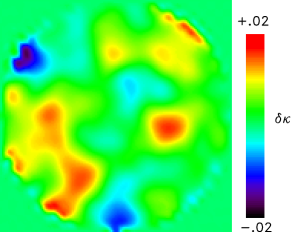
Figure 4: Convergence of the cluster smoothed with a $1^{\prime}$ Gaussian. Top panel: Input profile ; Middle panel: profile recovered from simulated ellipticities accounting for large scale structure. Bottom panel: The difference between the LSS estimator and the estimator which neglects LSS.

Mapmaking. One can also try to obtain information about the mass distribution in a cluster by inverting directly without assuming any particular profile. Since Kaiser and Squires first introduced this idea squireskaiser , many groups have worked to develop new techniques accounting for real world complications schneider . Here I simply want to discuss a way to improve an estimator by accounting for large scale structure. So, I will focus on one particular estimator hukeet , the so-called optimal estimator, used recently to make maps in CMB experiments mc . Although the maps made from this estimator are not particularly pretty, they do retain all the information stored in the likelihood function. Thus, they are very useful for quantitative analysis and they can be massaged in a number of ways (which I will not discuss here) to produce more realistic pictures. The main point is to see how much we can learn in the face of noise due to large scale structure.

The shear due to a cluster is linearly related to the convergance

$$\gamma^{\rm cl}_{\alpha}=K_{\alpha a}\kappa_{a}$$ (4)

where the index $a$ ranges over all pixels for which we are fitting the surface density. This presumably will be of order $N_{p}$ (but it does not have to be exactly equal to it, for we may choose to estimate the density in a coarser grid than the measured ellipticities). The kernel is

$$K_{\alpha a}=-{A\over\pi|\theta_{\alpha}-\theta_{a}|^{2}}\cases{\cos(2\phi)&$i=1$\cr-\sin(2\phi)&$i=2$}$$ (5)

where $\phi$ is the angle between the $x$-axis and the vector $\theta_{\alpha}-\theta_{a}$, and $A$ is the area of a pixel.

The measured shear is a combination of this signal, shape noise, and projections from large scale structure:$\gamma_{\alpha}=\gamma^{\rm cl}_{\alpha}+\gamma^{\rm shape}_{\alpha}+\gamma^{\rm lss}_{\alpha}.$ The latter two contributions have mean zero and a total covariance matrix $N$. Then the minimum variance estimator for the convergence is

$$\hat{\kappa}=C_{N}K^{t}N^{-1}\gamma$$ (6)

with mean equal to $\kappa^{\rm cl}$ and covariance matrix

$$C_{N}\equiv\left(K^{t}N^{-1}K\right)^{-1}.$$ (7)

Figure 4 shows the convergance of the cluster, along with the reconstruction accounting for large scale structure. Each of these was obtained from a pixelized set of ellipticities out to a radius of $15^{\prime}$ which included the signal due to the cluster, shape noise, and large scale structure. Fig. 2 shows the two noise sources. The map in the middle of Fig. 4 was obtained with the minimum variance estimate of equation [6].

The bottom panel of Fig. 4 shows the difference between a map which accounts for large scale structure and one that does not (i.e., one in which $N$ was set to $C^{\rm shape}$). Note especially that the minimum variance estimator obtains greater densities along a swath extending from the lower left to upper right. A comparison with the top panel shows that the minimum variance estimator more accurately reproduces the density. It does this by properly accounting for large scale structure. The estimator which neglects LSS treats the negative $\gamma_{t}$ swath from lower left to upper right in Fig. 2 as produced by the cluster. Thus, the total $\gamma_{t}$ it ascribes to the cluster is smaller than it should be. The result is an underprediction of the density along this swath. The minimum variance estimator avoids this pitfall.

How much does the variance go up when one uses the estimator which neglects large scale structure?

Figure 5: Uncertainty in the mass enclosed in an annulus of radius $\theta$ and width $1^{\prime}$ from estimators compared with the uncertainty in the absence of large scale structure. Dashed curve uses the equivalent of equation [6], without accounting for large scale structure.

Fig. 5 shows the errors on the mass within an annulus of radius $\theta$ compared with the errors if there was no large scale structure. As in the parametric estimation, we see that the minimum variance estimator more accurately determines the cluster mass. While the errors are larger than if there had been no large scale structure, they are significantly smaller than one gets when neglecting large scale structure.

This work is supported by the DOE, by NASA grant NAG5-10842, and by NSF Grant PHY-0079251. I am grateful to H. Hoekstra, C. Keeton, E. Rozo, and M. White for helpful comments.

References

- (1) J. P. Henry, Astrophys. J. 489, L1 (1997) ; P. T. P. Viana, and A. R. Liddle, Monthly Notices of Royal Astronomical Society 303, 535 (1999); T. H. Reiprich and H. Bohringer, Astrophys. J. 567, 716 (2002) ; V. R. Eke, S. Cole, and C. S. Frenk, Monthly Notices of Royal Astronomical Society 282, 263 (1996); N. A. Bahcall and X. Fan, Astrophys. J. 504, 1 (1998)
- (2) L. Wang and P. J. Steinhardt, Astrophys. J. 508, 483 (1998)
- (3) Z. Haiman, J. J. Mohr, and G. P. Holder, Astrophys. J. 553, 545 (2001)
- (4) In the case of optical richness, see, e.g., the theoretical investigations in M. P. van Haarlem, C. S. Frenk, and S. D. M. White, Monthly Notices of Royal Astronomical Society 287, 817 (1997); K. Reblinsky and M. Bartelmann, Astron. & Astrophys. 345, 1 (1999) ; M. White and C. S. Kochanek, Astrophys. J. 574, 24 (2002)
- (5) For a review see M. Bartelmann and P. Schneider, Physics Reports 340, 291 (2001). An incomplete list of weak lensing mass determinations is: J. A. Tyson, R. A. Wenk, and F. Valdes, Astrophys. J. 349, L1 (1990) ; Th. Erben et al., Astron. & Astrophys. 355, 23 (2000) ; D. Clowe et al., Astrophys. J. 539, 540 (2000) ; P. J. Marshall et al., Monthly Notices of Royal Astronomical Society 335, 1037 (2002).
- (6) C. A. Metzler, M. White, and C. Loken, Astrophys. J. 547, 560 (2001) ; M. White, L. van Waerbeke, and J. Mackey, Astrophys. J. 575, 640 (2002)
- (7) H. Hoekstra, Astron. & Astrophys. 370, 743 (2001) , Monthly Notices of Royal Astronomical Society 339, 1155 (2003)
- (8) J. F. Navarro, C. S. Frenk, and S. D. M. White, Monthly Notices of Royal Astronomical Society 275, 720 (1995), Astrophys. J. 490, 493 (1997)
- (9) where is the azumthal angle makes with a fixed -axis.
- (10) N. Kaiser and G. Squires, Astrophys. J. 404, 441 (1993) ; G. Squires and N. Kaiser, Astrophys. J. 473, 65 (1996) .
- (11) See, e.g., P. Schneider, astro-ph/0306465
- (12) W. Hu and C. R. Keeton, Phys. Rev. D 66, 063506 (2002)
- (13) See, e.g., S. Dodelson, Modern Cosmology (Academic Press, San Diego, 2003)