Abstract

We discuss a new mechanism which allows domain walls produced during the primordial electroweak phase transition. We show that the effective surface tension of these domain walls can be made vanishingly small due to a peculiar magnetic condensation induced by fermion zero modes localized on the wall. We find that in the perfect gas approximation the domain wall network behaves like a radiation gas. We consider the recent high-red shift supernova data and we find that the corresponding Hubble diagram is compatible with the presence in the Universe of a ideal gas of ferromagnetic domain walls. We show that our domain wall gas induces a completely negligible contribution to the large-scale anisotropy of the microwave background radiation.

1. Introduction

A considerable amount of interest has emerged in the physics of topological defects produced during cosmological phase transitions [1]. Indeed, even in a perfectly homogeneous continuous phase transition, defects will form if the transition proceeds sufficiently faster than the relaxation time of the order parameter [2, 3, 4, 5]. In such a non-equilibrium transition, the low temperature phase starts to form, due to quantum fluctuations, simultaneously and independently in many parts of the system. Subsequently, these regions grow together to form the broken-symmetry phase. When different causally disconnected regions meet, the order parameter does not generally match and a domain structure is formed.
In the standard electroweak phase transition the neutral Higgs field is the order parameter which is expected to undergo a continuum phase transition or a crossover [6, 7]. In the case in which the phase transition is induced by the Higgs sector of the Standard Model, the defects are domain walls across which the field flips from one minimum to the other. The defect density is then related to the domain size and the dynamics of the domain walls is governed by the surface tension $\sigma$. The existence of the domain walls, however, is still questionable. It was pointed out by Zel’dovich, Kobazarev and Okun [8] that the gravitational effects of just one such wall stretched across the universe would introduce a large anisotropy into the relic blackbody radiation. For this reason the existence of such walls was excluded. Quite recently, however, it has been suggested [9, 10] that the effective surface tension of the domain walls can be made vanishingly small due to a peculiar magnetic condensation induced by fermion zero modes localized on the wall. As a consequence, the domain wall acquires a non zero magnetic field perpendicular to the wall, and it becomes almost invisible as far as gravitational effects are concerned. In a similar way, even for the bubble walls, which are relevant in the case of first order phase transitions, it has been suggested [11] that strong magnetic fields may be produced as a consequence of non vanishing spatial gradients of the classical value of the Higgs field.
It is worthwhile to stress that in the realistic case where the domain wall interacts with the plasma, the magnetic field penetrates into the plasma over a distance of the order of the penetration length, which at the epoch of the electroweak phase transition is about an order of magnitude greater than the wall thickness. This means that fermions which scatter on the wall feel an almost constant magnetic field over a spatial region much greater than the wall thickness.
In this paper we consider thin domain walls eventually produced during the primordial electroweak phase transition. We focus on domain walls where the magnetic condensation induced by fermion zero modes leads to ferromagnetic domain walls (in the following FDW). Obviously, ferromagnetic domain walls are not topological stable. However, FDWs are characterized by the vanishing of the effective surface tension. As a consequence FDWs are dynamically stable structures, due to a huge energy barrier against spontaneous decays, which could have survived until today.
The plan of the paper is as follows. In Section II we consider FDW in the thin wall approximation and discuss the general properties of the associated energy-momentum tensor. In Section III we evaluate the energy momentum tensor contributions due to positive energy fermions captured by the domain wall. In Section IV we discuss the equation of state of a domain-wall network in the ideal gas approximation. In Section V we discuss the gravitational properties of the ideal gas of FDWs. Section VI is devoted to the analysis of the temperature anisotropy on the Cosmic Microwave Background Radiation induced by the ferromagnetic domain wall network. Finally, we summarize our results in Section VII. Some technical details are relegated in the Appendix.

2. The energy-momentum tensor of a FDW

Topologically stable kinks are ensured when the vacuum manifold ${\cal M}$, the space of all accessible vacua of the theory, is disconnected, i.e. $\pi_{0}({\cal M})$ is nontrivial.
We shall consider a simplified model in which the kink is a infinitely static domain wall in the $(x,y)$ plane in a flat space-time. That is we assume that the vacuum manifold consists of just two disconnected components and restrict ourselves to one spatial dimension. In our model the scalar sector that give rise to a planar wall is given by a real scalar field with density Lagrangian,

$${\cal L}_{\phi}=\frac{1}{2}\,\partial^{\mu}{\phi}\,\partial_{\mu}{\phi}\,-V(|\phi|,T).$$ (2.1)

Lagrangian (2.1) has an exact $Z_{2}$ symmetry corresponding to the discrete transformation $\phi\rightarrow-\phi$. At zero temperature the $Z_{2}$ symmetry is spontaneously broken, with $\phi$ acquiring a vacuum expectation of order $v$. In the tree approximation, the set of vacuum states is $\langle\,\phi\,\rangle^{2}=v^{2}$ so that $\pi_{0}({\cal M})\neq 0$. Then, if we apply boundary conditions that the vacuum at $-\infty$ lie in $-v$ and that at $+\infty$ lie in $+v$, by continuity there must exists a region in which the scalar field is out of the vacuum. This region is a domain wall. If we take the potential at zero temperature as $V(\phi)=\frac{\lambda}{4}({\phi}^{2}-v^{2})^{2}$, it is easy to see that the classical equation of motion admits the solution describing the transition layer between two regions with different values of $\langle\,\phi\,\rangle$,

$$\phi(z)=v\,\tanh(z/\Delta),$$ (2.2)

where $\Delta=\sqrt{2}\lambda^{-1/2}\,v^{-1}$ is the thickness of the wall.
The energy-momentum tensor for the $\phi$-kink (2.2) is,

$$T_{(\phi)\;\nu}^{\mu}=\alpha(z)\,\sigma_{\phi}\;diag\,(1,1,1,0),$$ (2.3)

$$\alpha(z)=\frac{3}{4\Delta}\,[\,\cosh{(z/{\Delta})}]^{-4},$$ (2.4)

where

$$\sigma_{\phi}=\int_{-\infty}^{+\infty}dz\,T_{(\phi)\;0}^{0}=\frac{2\sqrt{2}}{3}\lambda^{1/2}v^{3}$$ (2.5)

is the surface energy density associated with the scalar field. In the thin wall approximation, i.e. $\Delta\rightarrow 0$, $\alpha(z)$ reduces to a $\delta$-function. Unless the symmetry breaking scale $v$ is very small, surface density energy of the kink is extremely large and implies that cosmological domain walls would have an enormous impact on the homogeneity of the Universe. A stringent constraint on the wall tension $\sigma_{\phi}$ for a $Z_{2}$-wall can be derived from the isotropy of the microwave background. If the interaction of walls with matter is negligible, then there will be a few walls stretching across the present horizon. They introduce a fluctuation in the temperature of the microwave background of order $\delta T/T\sim G_{N}\,\sigma_{\phi}\,t_{0}$, where $t_{0}$ is the present time. Observations constrain $\delta T/T\,<\,10^{-5}$, and thus models predicting topologically stable domain walls with $v\,>\,1\;MeV$ should be ruled out.
On the other hand, we are interested in domain walls formed during the electroweak phase transition by the Kibble-Zurek mechanism [2, 3, 4, 5]. Even these domain walls are approximately accounted for by Eq. (2.2), so that the energy-momentum tensor is given by Eq. (2.3). Since $v\,\sim\,10^{2}\;GeV$, it is widely believed that there must be some provision for the elimination of these defects which indeed are not topological stable. However, quite recently it has been suggested that the effective surface tension of the domain wall can be made vanishingly small due to a peculiar magnetic condensation induced by fermion zero modes localized on the wall. As a consequence the domain wall acquires a non zero magnetic field perpendicular to the wall. This mechanism is able to make these defects almost dynamical stable. Indeed, FDWs are protected against decay by a huge energy barrier.
In general, for a FWD the magnetic field vanishes in the regions where the scalar condensate is constant. So that, the magnetic field can be different from zero only in the regions where the scalar condensate varies, $i.e.$ in a region of the order of the wall thickness. However, it is worthwhile to stress that in the realistic case where the domain wall interacts with the plasma, the magnetic field penetrates into the plasma over a distance of the order of the penetration length which at the time of electroweak phase transition is about an order of magnitude greater than the wall thickness. This means that fermions interacting with the wall feel an almost constant magnetic field over a spatial region much greater than the wall thickness. So that as concern the interaction of fermions with FWDs, we can assume that the magnetic field is almost constant.
For completeness, let us briefly review the generation of ferromagnetic domain walls at the electroweak phase transition [9]. After the electroweak spontaneous symmetry breaking the unique long range gauge field is the electromagnetic field $A_{\mu}$. In our scheme the real scalar field is the physical Higgs field, so that $A_{\mu}$ does not couple directly to $\phi$. The electromagnetic Lagrangian is:

$${\cal L}_{em}=-\frac{1}{4}F_{\mu\nu}\,F^{\mu\nu}.$$ (2.6)

We are interested in the case of an external magnetic field $B$ (localized on the wall at $z=0$) directed along the $z$-direction,

$$A_{\mu}=(0,0,-Bx,0),$$ (2.7)

where without loss of generality we may consider $B>0$. Assuming that the magnetic field $B$ is localized on the wall, we can write,

$$T_{(B)\;\nu}^{\mu}(z)=\beta(z)\,\sigma_{B}\;diag\,(1,-1,-1,0),$$ (2.8)

where

$$\sigma_{B}=\int_{-\infty}^{+\infty}\!dz\,T_{(B)\;0}^{0}=\Delta\frac{B^{2}}{2}$$ (2.9)

is the surface energy density associated with the magnetic field if $B$ is sizable over a distance $z\sim\Delta$, and $\beta(z)$ is a localization function of $B$ on the wall. In the thin wall approximation we expect that $\beta(z)$ reduces to a $\delta$-function.
Next we consider a four dimensional massless Dirac fermion coupled to the scalar field through the Yukawa coupling, and in presence of the homogeneous background magnetic field (2.7). The Dirac fermion $\psi$ is described by the Lagrangian:

$${\cal L}_{\psi}={\bar{\psi}}(i\,/\!\!\!\partial-e\;/\!\!\!\!\!\>\!A-g_{Y}\,\phi)\,\psi$$ (2.10)

where we consider $e>0$. In presence of the kink (2.2) the Dirac equation,

$$(i\,/\!\!\!\partial-e\;/\!\!\!\!\!\>\!A-g_{Y}\,\phi)\,\psi=0,$$ (2.11)

admits solutions localized on the wall [9]. Using the following representation of the Dirac algebra,

$$\alpha=0,1,2\,:\;\gamma\,^{\alpha}=\left(\begin{array}[]{cc}\stackrel{{\scriptstyle\sim}}{{\gamma}}\!\!\,^{\alpha}&0\\ 0&-\stackrel{{\scriptstyle\sim}}{{\gamma}}\!\!\,^{\alpha}\end{array}\right)\!,\;\;\;\;\gamma\,^{3}=\left(\begin{array}[]{cc}0&i\\ i&0\end{array}\right)\!,$$ (2.12)

with

$$\stackrel{{\scriptstyle\sim}}{{\gamma}}\!\!\,^{0}=\sigma_{3},\;\;\stackrel{{\scriptstyle\sim}}{{\gamma}}\!\!\,^{1}=i\,\sigma_{1},\;\;\stackrel{{\scriptstyle\sim}}{{\gamma}}\!\!\,^{2}=i\,\sigma_{2},$$ (2.13)

where $\sigma_{i}$ are the usual Pauli matrices, we find for the localized modes [9],

$$\psi(x,y,z,t)=\frac{1}{\sqrt{2}}\,\omega(z)\left(\begin{array}[]{c}\rho(x,y,t)\\ \rho(x,y,t)\end{array}\right),$$ (2.14)

$$\omega(z)=N\,[\,\cosh{(z/{\Delta})}]^{-\xi\Delta},$$ (2.15)

where $\xi=g_{Y}\,v$ is the mass which the fermion acquires in the broken phase, $\rho(x,y,t)$ is a Pauli spinor that satisfies the $(2+1)$-dimensional massless Dirac equation in a constant external magnetic field, and $N$ is a normalization constant given by

$$N=\left[\>\int_{-\infty}^{+\infty}\!\!dz\,\omega^{2}(z)\right]^{-1/2}\!=\>\left[\Delta\,\mbox{B}(\xi\,\Delta,1/2)\right]^{-1/2},$$ (2.16)

B$(x\,,y)$ being the Euler Beta function.
Let us consider the energy-momentum tensor of the four dimensional massless Dirac fermion, $T^{\mu}_{(\psi)\,\nu}$. It is straightforward to show that the non-zero components are given by:

$$T^{\alpha}_{(\psi)\,\beta}=i\,\omega^{2}(z)\rho^{{\dagger}}\stackrel{{\scriptstyle\sim}}{{\gamma}}\!\!\,^{0}\stackrel{{\scriptstyle\sim}}{{\gamma}}\!\!\,^{\alpha}\,\partial_{\beta}\rho,$$ (2.17)

$$T^{\alpha}_{(\psi)\,3}=-i\,g_{Y}\,\phi(z)\omega^{2}(z)\rho^{{\dagger}}\stackrel{{\scriptstyle\sim}}{{\gamma}}\!\!\,^{0}\stackrel{{\scriptstyle\sim}}{{\gamma}}\!\!\,^{\alpha}\rho.$$ (2.18)

In the thin-wall approximation $\omega^{2}(z)$ reduces to a $\delta$-function so that $T^{\alpha}_{(\psi)\,3}$ goes to zero. Therefore the tensor reduces to:

$$T_{(\psi)\;\nu}^{\,\mu}(x,y,z)=\delta(z)\,\left(\begin{array}[]{cc}T_{(\rho)\;\beta}^{\,\alpha}(x,y)&\;\;0\\ \\ 0&\;\;0\end{array}\right),$$ (2.19)

where $T_{(\rho)\beta}^{\,\alpha}=i\rho^{\dagger}\stackrel{{\scriptstyle\sim}}{{\gamma}}\!\!^{0}\stackrel{{\scriptstyle\sim}}{{\gamma}}\!\!^{\alpha}\partial_{\beta}\rho$ is the energy-momentum tensor for a $(2+1)$-dimensional massless Dirac fermion coupled to the magnetic field.
The resulting energy-momentum tensor of the wall is given by

$$T_{(w)\;\nu}^{\mu}=T_{(\phi)\;\nu}^{\mu}+T_{(B)\;\nu}^{\mu}+T_{(\psi)\;\nu}^{\mu}.$$ (2.20)

¿From Eq. (2.19) we see that the $(3+1)$-dimensional tensor $T^{\mu}_{(\psi)\,\nu}$ is obtained by evaluating $T_{(\rho)\beta}^{\,\alpha}$ which corresponds to $(2+1)$-dimensional Dirac fermions localized on the wall.
It is known since long time that in $(2+1)$-dimensional QED in presence of un external homogeneous background magnetic field with massless Dirac fermions it is energetically favorable the spontaneous generation of a negative mass term [12]. So we are lead to consider the following effective $(2+1)$-dimensional Dirac equation:

$$(i\stackrel{{\scriptstyle\sim}}{{\gamma}}\!\!^{\alpha}\partial_{\alpha}-e\stackrel{{\scriptstyle\sim}}{{\gamma}}\!\!^{\alpha}A_{\,\alpha}-m)\,\rho(x,y,t)=0.$$ (2.21)

Taking $\rho(x,y,t)=e^{-iEt}\,\rho(x,y)$ we get [12]

$$E=+E_{n}\,:\;\;\;\rho_{n,p}^{(+)}=\left(\frac{E_{n}+m}{2E_{n}}\right)^{1/2}\frac{e^{ipy}}{\sqrt{2\pi}}\;e^{-\zeta^{2}/2}\,\left(\begin{array}[]{c}N_{n}\,H_{n}(\zeta)\\ \\ -\frac{(E_{n}^{2}-m^{2})^{1/2}}{E_{n}+m}\,N_{n-1}\,H_{n-1}(\zeta)\end{array}\right)\!,$$ (2.22)

$$E=-E_{n}\,:\;\;\;\rho_{n,p}^{(-)}=\left(\frac{E_{n}-m}{2E_{n}}\right)^{1/2}\frac{e^{ipy}}{\sqrt{2\pi}}\;e^{-\zeta^{2}/2}\,\left(\begin{array}[]{c}N_{n}\,H_{n}(\zeta)\\ \\ \frac{(E_{n}^{2}-m^{2})^{1/2}}{E_{n}+m}\,N_{n-1}\,H_{n-1}(\zeta)\end{array}\right)\!,$$ (2.23)

$$E=E_{0}=m\,:\;\;\;\rho_{0,p}=N_{0}\,\frac{e^{ipy}}{\sqrt{2\pi}}\;e^{-\zeta^{2}/2}\,\left(\begin{array}[]{c}1\\ 0\end{array}\right)\!,$$ (2.24)

where

$$E_{n}\!\! = \!\!\sqrt{2neB+m^{2}}\;,$$ (2.25)

$$\zeta\!\! = \!\!\sqrt{eB}\left(x-\frac{p}{eB}\right),$$ (2.26)

$$N_{n}\!\! = \!\!\left(\frac{eB}{\pi}\right)^{1/4}\frac{1}{\sqrt{2^{n}\,n!}}\,,$$ (2.27)

with $n=1,2,...$, and $H_{n}(x)$ are Hermite polynomials. The normalization is

$$\int\!\!\ d^{2}x\;\rho_{n,p}^{(\pm)\;{\dagger}}({\bf x})\,\rho_{n^{\prime},p^{\prime}}^{(\pm)}({\bf x})=\delta(p-p\,^{\prime})\,\delta_{nn^{\prime}}\,.$$ (2.28)

It is convenient to expand the fermion field operator $\rho$ in terms of $\rho_{n,p}^{(+)}$ and $\rho_{n,p}^{(-)}$. In other words, we adopt the so-called Furry’s representation. For negative mass term we have:

$$\rho\;=\;\sum_{n=0}^{\infty}\int_{-\infty}^{+\infty}\!\!dp\;a_{n\,p}\,\rho_{n,p}^{(+)}\;+\;\sum_{n=1}^{\infty}\int_{-\infty}^{+\infty}\!\!dp\;b_{n\,p}^{\dagger}\,\rho_{n,p}^{(-)}\;.$$ (2.29)

We observe that in the case of negative mass the positive solutions have eigenvalues $+E_{n}$ with $n\geq 1$ and the negative ones $-E_{n}$ with $n\geq 0$. In the expansion of $\rho$ we associate particle operators to positive energy solutions and antiparticle operators to negative energy solutions. These operators satisfy the standard anticommutation relations,

$$\{a_{n\,p}\;,a_{n^{\prime}\,p^{\prime}}^{\dagger}\}=\{b_{n\,p}\;,b_{n^{\prime}\,p^{\prime}}^{\dagger}\}=\delta_{n\,n^{\prime}}\,\delta(p-p\,^{\prime}),$$ (2.30)

others anticommutators being zero. The energy-momentum tensor operator is

$$T_{(\rho)\;\beta}^{\,\alpha}=i\,\rho^{\dagger}\,\stackrel{{\scriptstyle\sim}}{{\gamma}}\!\!\,^{0}\stackrel{{\scriptstyle\sim}}{{\gamma}}\!\!\,^{\alpha}\,\partial_{\beta}\;\rho.$$ (2.31)

We need the surface density of the vacuum expectation value of energy-momentum tensor operator defined as:

$$\langle\,T_{(\rho)\;\beta}^{\,\alpha}\,\rangle=\frac{1}{A}\int d^{2}\,x\,\frac{\langle 0|\,T_{(\rho)\;\beta}^{\,\alpha}\,|0\rangle}{\langle 0|0\rangle}\,,$$ (2.32)

where $A$ is the area of the wall and $|0\rangle$ is the fermion vacuum. In the Furry’s representation $\langle\,T_{(\rho)\;\beta}^{\,\alpha}\,\rangle$ reads

$$\langle\,T_{(\rho)\;\beta}^{\,\alpha}\,\rangle=\frac{1}{A}\int\!d^{2}x\,\sum_{n=0}^{\infty}\,\int_{-\infty}^{+\infty}\!\!dp\;\rho_{n,p}^{(-)\,\dagger}\;i\stackrel{{\scriptstyle\sim}}{{\gamma}}\!\!\,^{0}\stackrel{{\scriptstyle\sim}}{{\gamma}}\!\!\,^{\alpha}\,\partial_{\beta}\;\rho_{n,p}^{(-)}\;.$$ (2.33)

for the negative mass theory. Inserting Eqs. (2.23) and (2.24) into Eq. (2.33), it is straightforward to obtain

$$\sigma_{\rho}\! \equiv \!\langle\,T_{(\rho)\;0}^{\,0}\,\rangle\;=\;-\frac{eB}{2\pi}\sum_{n=0}^{\infty}E_{n},$$ (2.34)

$$-p_{\rho}\! \equiv \!\langle\,T_{(\rho)\;1}^{\,1}\,\rangle\;=\;\langle\,T_{\rho\;2}^{\,2}\,\rangle\;=\;\frac{{(eB)}^{2}}{2\pi}\sum_{n=0}^{\infty}\frac{n}{E_{n}}\,,$$ (2.35)

while all other $\langle\,T_{(\rho)\;\beta}^{\,\alpha}\,\rangle$ are equal to zero. Therefore, the energy-momentum tensor is:

$$\langle\,T_{(\rho)\;\beta}^{\,\alpha}\,\rangle=diag\,(\sigma_{\rho},-p_{\rho},-p_{\rho}),$$ (2.36)

where $\sigma_{\rho}\,$ and $\,p_{\rho}$ are the surface density energy and pressure of the fermionic condensate, respectively. It easy to show that the following relation

$$p_{\rho}=B\frac{\partial\sigma_{\rho}}{\partial B}-\sigma_{\rho}$$ (2.37)

holds. We shall consider the “effective” energy-momentum tensor defined as:

$$\langle\,T_{(\rho)\;\beta}^{\alpha}\,\rangle_{eff}\,=\,\langle\,T_{(\rho)\;\beta}^{\alpha}\,\rangle_{B}\;-\langle\,T_{(\rho)\;\beta}^{\alpha}\,\rangle_{B=0}\,.$$ (2.38)

By using the integral representation

$$\sqrt{a}=-\int_{0}^{\infty}\!\frac{ds}{\sqrt{\pi s}}\frac{d}{ds}\,e^{-as},$$ (2.39)

introducing the dimensionless variable $\,\eta=eB/{m^{2}}\,$ and the function

$$g(\eta)=\int_{0}^{\infty}\!\frac{ds}{\sqrt{\pi s}}\frac{d}{ds}\,e^{-s/{\eta}}\left[\frac{1}{1-e^{-2s}}-\frac{1}{2s}\right]\!,$$ (2.40)

we cast Eq. (2.38) into

$$\sigma_{\rho}^{eff}\! \equiv \!\langle\,T_{(\rho)\;0}^{0}\,\rangle_{eff}\;=\;\delta(z)\,\frac{(eB)^{3/2}}{2\pi}\,g(\eta),$$ (2.41)

$$-p_{\rho}^{eff}\! \equiv \!\langle\,T_{(\rho)\;1}^{1}\,\rangle_{eff}\;=\;\langle\,T_{(\rho)\;2}^{2}\,\rangle_{eff}\;=\;-\delta(z)\,\frac{(eB)^{3/2}}{2\pi}\,\left[\frac{1}{2}\,g(\eta)+\eta\,\frac{\partial g(\eta)}{\partial\eta}\right]\!.$$ (2.42)

Taking into account Eqs. (2.20), (2.41), (2.42), the final expression of the effective energy-momentum tensor of a thin FDW is:

$$\langle\,T_{(w)\;\nu}^{\mu}\,\rangle=\delta(z)\,diag\left(\,\sigma_{w}\,,\,-p_{w}\,,\,-p_{w}\,,0\right),$$ (2.43)

where

$$\sigma_{w}\!\! = \!\!\sigma_{\phi}+\sigma_{B}+\sigma_{\rho}^{eff},$$ (2.44)

$$p_{w}\!\! = \!\!-\sigma_{\phi}+\sigma_{B}+p_{\rho}^{eff}.$$ (2.45)

We are interested on the value of $\langle T^{\mu}_{(w)\,\nu}\rangle$ for the magnetic field $B^{*}$ that minimizes the energy density $\sigma_{w}$. As shown in Ref. [9] the magnetic field $B^{*}$ can be approximated by:

$$B^{*}=\frac{e|m|^{2}}{4\pi}\frac{1}{|m|\Delta+\frac{e^{2}}{12\pi}}\;.$$ (2.46)

Moreover the stability condition

$$\sigma_{w}=0$$ (2.47)

gives in turns the value of $|m^{*}|$. Equation (2.47) assures that our ferromagnetic domain walls have a vanishing effective surface tension. Moreover, it is remarkable that Eq. (2.47) implies:

$$p_{w}(B^{*},|m|^{*})=0\;.$$ (2.48)

Note that Eq. (2.48) is an exact consequence of the stability condition Eq. (2.47) and does not rely on the approximate expression for $B^{*}$ given by Eq. (2.46). By using the standard values $v\simeq 250\!$ GeV, $\alpha_{QED}=e^{2}/4\pi\simeq 1/137$ and assuming $\lambda\simeq 0.5$ we obtain from Eqs. (2.46) and (2.47) the following value of the magnetic field [9],

$$B^{*}\simeq 5.0\;10^{24}\,\mbox{Gauss}.$$ (2.49)

Interestingly enough, such a value of the magnetic field at the primordial electroweak phase transition could be relevant for the generation of the primordial magnetic field [13].
It is worthwhile to stress that Eqs. (2.47) and (2.48) imply that our ferromagnetic domain walls are almost invisible as concern the gravitational effects. However, as already discussed, in the realistic case where the domain wall interacts with the plasma, the magnetic field penetrates into the plasma over a distance of the order of the penetration length $\lambda$ which is about an order of magnitude greater than $\Delta$. It follows that the above estimate of the induced magnetic field at the electroweak scale $B^{*}$ is reduced by a factor $\sqrt{\frac{\Delta}{\lambda}}\,\sim\,0.3$ which is still of cosmological interest [14]. Moreover, on the ferromagnetic domain walls there are also positive energy states. As a consequence fermions incident on the wall with an energy equal to the empty states can be trapped on the wall giving a non trivial contribution to the energy-momentum tensor. Thus, in order to investigate the gravitational properties of the ferromagnetic domain walls it is important to take care of these contributions to the energy-momentum tensor.

3. The energy-momentum tensor of a massive FDW

On the wall there are also available positive energy bounded states. Therefore when incident fermions have the same energy as the allowed bounded states on the wall, they could be captured. In this case, the fermions bounded to the ferromagnetic domain wall do contribute to the energy-momentum tensor of the wall. In the following we shall refer to FDW bounded with positive-energy fermions as massive FDW. In this Section we calculate the energy-momentum tensor of massive FWDs.
To discuss the localized solutions with positive energy we rewrite Eq. (2.11) as:

$$(i\,/\!\!\!\partial-e\;/\!\!\!\!\!\>\!A-\xi\,g)\,\psi(x,y,z,t)=0,$$ (3.1)

where $\xi=g_{Y}\,v$, $\,g(z)=\tanh(\frac{z}{\Delta})$ and $\psi(x,y,z,t)$ is the wave function of the fermion eventually captured by the FDW and having positive energy corresponding to a allowed bound state on the wall. For reader convenience we relegate in the Appendix the details of our calculations. As shown in the Appendix, the wave functions of the localized fermionic modes are given by:

$$\psi^{1}_{+e} = N\,A_{n}\,e^{-\frac{\xi^{2}}{2}+i\,p_{y}\,y-i\,E\,t}(\cosh\frac{z}{\Delta})^{-\xi\,\Delta}\,[H_{n}\,E\,u^{1}_{+}+2\,n\,\sqrt{|eB|}\,H_{n-1}\,u^{2}_{+}\,],$$ (3.2)

$$\psi^{2}_{+e} = N\,A_{n-1}\,e^{-\frac{\xi^{2}}{2}+i\,p_{y}\,y-i\,E\,t}(\cosh\frac{z}{\Delta})^{-\xi\,\Delta}\,[H_{n-1}\,E\,u^{2}_{+}+\sqrt{|eB|}\,H_{n}\,u^{1}_{+}\,],$$ (3.3)

$$\psi^{1}_{-e} = N\,A_{n-1}\,e^{-\frac{\xi^{2}}{2}+i\,p_{y}\,y-i\,E\,t}(\cosh\frac{z}{\Delta})^{-\xi\,\Delta}\,[H_{n-1}\,E\,u^{1}_{+}-\sqrt{|eB|}\,H_{n}\,u^{2}_{+}\,],$$ (3.4)

$$\psi^{2}_{-e} = N\,A_{n}\,e^{-\frac{\xi^{2}}{2}+i\,p_{y}\,y-i\,E\,t}(\cosh\frac{z}{\Delta})^{-\xi\,\Delta}\,[H_{n}\,E\,u^{2}_{+}-2\,n\,\sqrt{|eB|}\,H_{n-1}\,u^{1}_{+}\,],$$ (3.5)

where $N$ is the normalization constant evaluated in the Appendix, and

$$E_{n}=\sqrt{2\,n\,|e|\,B},\,\,\,\,\,\,\,n=1,2,...$$ (3.6)

The wave functions (3.2), (3.3) correspond to fermions, while (3.4), (3.5) to antifermions. Note that fermions have spin parallel to the magnetic field, while antifermions have spin antiparallel to the magnetic field.
In a previous paper [15] we investigated the scattering of fermions off walls in presence of a constant magnetic field . In particular, we discussed fermion states corresponding to solutions of Dirac equation (2.11) which are localized on the domain wall. We found that there is total reflection for fermions with parallel and antiparallel spin at energies $E_{n}^{2}\,-\,\xi^{2}=2\,n\,|e|\,B$ and $E_{n}^{2}\,-\,\xi^{2}=2\,(n+1)\,|e|\,B$, respectively. Note that the difference is due to the fermion mass term $\xi$ which, indeed, vanishes on the wall where the system is in the symmetric phase. ¿From the physical point of view, we see that fermions with asymptotically positive kinetic energy equal to $\sqrt{2\,n\,|e|\,B}$ for parallel spin, and $\sqrt{2\,(n+1)\,|e|\,B}$ for antiparallel spin, can be indeed trapped on the domain wall. As a consequence, we see that ferromagnetic domain walls immersed into the primordial plasma are able to capture fermions by filling the Landau levels up to $n\,=\,N_{max}$. Obviously, $N_{max}$ depends on the plasma temperature $T$, for we must have $E_{n}\;\lesssim\;T$. In our case, the temperature at the electroweak phase transition is of the order of $10^{2}\;GeV$. Taking into account Eqs. (2.49) and (3.6) we get $N_{max}\;\backsimeq\;1$.
Let us indicate with $|w\rangle$ the generic massive FDW, namely a ferromagnetic domain wall filled with fermions ($+e$) and antifermions ($-e$), with “spin up” ($s=1$) and “spin down” ($s=2$) respectively, up to Landau level $N_{max}$ . Thus, the expectation value of the energy-momentum tensor on the state $|w\rangle$ is:

$$\langle T^{\mu}_{(\Psi)\,\nu}\rangle=\frac{1}{A}\int d^{2}x\,\frac{\langle\,w|T^{\mu}_{(\psi)\,\nu}|w\,\rangle}{\langle w|w\rangle}\,,$$ (3.7)

where

$$T^{\mu}_{(\Psi)\,\nu}=i\,{\bar{\Psi}}\gamma^{\mu}\partial_{\nu}\Psi\;.$$ (3.8)

To evaluate $\langle T^{\mu}_{(\Psi)\,\nu}\rangle$ we expand the fermionic operator $\Psi$ in terms of the states (3.2)-(3.5) as follows

$$\Psi=\sum_{n_{s}}\sum_{s}\int dp_{y}\,[\,a(u_{s},p_{y},s)\,\psi_{+e}^{s,n_{s},p_{y}}+b^{{\dagger}}(u_{s},p_{y},s)\,\psi^{s,n_{s},p_{y}}_{-e}\,].$$ (3.9)

In the thin wall approximation we find,

$$\langle T^{\mu}_{(\Psi)\,\nu}(z)\rangle=\delta(z)\,\sigma_{\Psi}\,diag(1,-1/2,-1/2,0),$$ (3.10)

where

$$\sigma_{\Psi}=\int d\,z\,\langle T^{0}_{(\Psi)\,0}(z)\rangle=\frac{2\,|e\,B^{*}|^{3/2}}{\pi}\,\sum_{n=1}^{N_{max}}\sqrt{n}\;\backsimeq\;\frac{2\,|e\,B^{*}|^{3/2}}{\pi}\,.$$ (3.11)

Taking into account the value of $B^{*}$ given in Eq. (2.49), we see that Eq. (3.11) implies that $\sigma_{\Psi}$ is comparable to $\sigma_{\phi}$ given by Eq. (2.5), so that massive FDWs could display important gravitational effects which, eventually, could be in contrast with observations. Indeed, the cosmological electroweak phase transition should lead to a network of domain walls. However, solving for the cosmic evolution of a domain-wall network is quite involved. Nevertheless some essential features can studied by considering the dynamic of the domain-wall network in the ideal gas approximation [17].

4. Ideal gas of FDWs

In this Section we shall follow quite closely the analysis of Ref. [17] to calculate the equation of state for a ideal gas of massive ferromagnetic domain walls.
Let us consider a perfect gas of walls moving with velocity $v$ in a box of volume $V\;\gg\;\xi$, where $\xi$ is a typical distance between walls. The perfect gas approximation amounts to neglect any dissipative effects due to the interaction of the walls. We first consider a planar wall in the $x-y$ plane. Because of the symmetry, the energy-momentum tensor will be a function only of $z$. Following Ref. [17] we find that the average energy-momentum tensor of the wall gas is:

$$\langle T^{\mu\nu}_{(w)}\rangle\sim\frac{1}{\langle L\rangle}\int\!dz\;T^{\mu\nu}_{(w)}(z)\equiv\frac{1}{\langle L\rangle}W^{\mu\nu}.$$ (4.1)

where $T^{\mu\nu}_{(w)}$ is given by Eqs. (3.10) and (3.11) for massive FDWs, and $\langle L\rangle$ is the average wall separation. If the walls are moving with average velocity $v$ in the $+\,\hat{z}$ direction, we can obtain the energy-momentum tensor by boosting $W^{\mu\nu}$ in $z$-direction. Repeating the procedure for walls moving in the $-\,\hat{z}$, $\pm\,\hat{x}$, $\pm\,\hat{y}$ directions and averaging over the walls, we see that the average energy-momentum tensor for an ideal gas of massive FDWs is diagonal. Moreover, we have:

$$\rho_{w} \!\!\equiv\!\! \langle T^{00}_{(w)}\rangle=\frac{\sigma_{w}}{\langle L\rangle}\gamma^{2},$$ (4.2)

$$p_{w} \!\!\equiv\!\! \langle T^{11}_{(w)}\rangle=\langle T^{22}_{(w)}\rangle=\langle T^{33}_{(w)}\rangle=\frac{1}{3}\,\rho_{w}\,,$$ (4.3)

where $\gamma=\left(1-v^{2}\right)^{-1/2}$ is the Lorentz factor and $v$ is the mean velocity of a wall. In Eq. (4.2) $\sigma_{w}$, the surface energy density for a massive FDW, is given by Eq. (3.11). From Eq. (4.3) we see that the equation of state for a ideal gas of massive FDWs does not depend on the wall velocity and coincides with the equation of state of a radiation gas.

It is clear that in the more realistic case in which the walls interact with the primordial plasma the equation of state for a gas of massive FDWs is expected to be more stiff than that of a radiation gas. Writing the pressure as $p_{w}=\alpha\rho_{w}$ we expect that $\alpha<1/3$ in the primordial Universe (say before the time of structure formation). On the other hand, at the present time the dissipative effects due to the interaction of the walls can be safely neglected and then the perfect gas approximation holds.

In the following we shall work in the ideal case of non-interacting walls since we will concentrate on physical process occurred at relatively recent times (i.e. after the beginning of structure formation).

5. Large scale gravitational properties

In a recent paper we investigated the gravitational properties of thin planar massive ferromagnetic domain walls in the weak field approximation [18]. In order to understand the cosmological implications of FDWs we must consider the standard model of the Universe which is based upon the Friedmann-Robertson-Walker cosmological model [17]. The Friedmann-Lemaitre equations for the expansions parameter $R$ are:

$$\frac{{\stackrel{{\scriptstyle\cdot}}{{R}}}{\,{}^{2}}}{R^{2}}+\frac{k}{R^{2}}=\frac{8\pi G_{N}}{3}\,\rho_{tot}\,+\,\frac{\Lambda}{3},$$ (5.1)

$$2\frac{\stackrel{{\scriptstyle\cdot\cdot}}{{R}}}{R}+\frac{{\stackrel{{\scriptstyle\cdot}}{{R}}}{\,{}^{2}}}{R^{2}}+\frac{k}{R^{2}}=-8\pi G_{N}\,p_{tot}\;+\;\Lambda\;,$$ (5.2)

where $\stackrel{{\scriptstyle\cdot}}{{R}}=dR/dt$ is the derivative respect to the cosmic time $t$, $k$ is the curvature constant ( $k$ equals to $-1,\,0,\,+1$ for a Universe which is respectively open, flat, and closed), and $\Lambda$ is the cosmological constant. Equation (5.1) tells us that there are three competing terms which drive the expansion: a term of energy (matter and radiation), the cosmological constant, and a curvature term. Recent observations on temperature anisotropy of the cosmic microwave background [19, 20, 21] strongly indicate that the Universe geometry is very close to flat. So that, in the following we assume $k\,=\,0$. We are interested in the matter-dominated Universe where the radiation energy density and the matter pressure are negligible. Allowing for a FDW gas with density $\rho_{w}$ and pressure $p_{w}$ related by the equation of state Eq. (4.3), the Friedmann-Lemaitre equations become:

$$H^{2}\;=\;\frac{8\pi G_{N}}{3}\,(\rho_{m}\,+\,\rho_{w})\,+\,\frac{\Lambda}{3},$$ (5.3)

$$2\frac{\stackrel{{\scriptstyle\cdot\cdot}}{{R}}}{R}+\;H^{2}\;=\;-8\pi G_{N}\,p_{w}\;+\;\Lambda\;,$$ (5.4)

where

$$H\;=\;\frac{\stackrel{{\scriptstyle\cdot}}{{R}}}{R}$$ (5.5)

is the Hubble parameter. By introducing the following $\Omega$-functions:

$$\Omega_{m} \!\!\equiv\!\! \frac{\rho_{m}}{\rho_{c}}\,,$$ (5.6)

$$\Omega_{w} \!\!\equiv\!\! \frac{\rho_{w}}{\rho_{c}}\,,$$ (5.7)

$$\Omega_{\Lambda} \!\!\equiv\!\! \frac{\Lambda}{3H^{2}},$$ (5.8)

where $\rho_{c}\equiv 3H^{2}/8\pi G_{N}$ is the critical density, we cast Eq. (5.3) in the form:

$$\Omega_{m}+\Omega_{w}+\Omega_{\Lambda}=1.$$ (5.9)

By defining the following dimensionless variables:

$$\tau \!\!\equiv\!\! t/t_{0}\,,$$ (5.10)

$$r \!\!\equiv\!\! R/R_{0}\,,$$ (5.11)

where the index $0$ refers to the present time, and using Eq. (4.3), the equation of state for the ideal gas of FDW, we write Eq. (5.4) in the form:

$$\left(\frac{dr}{d\tau}\right)\;=\;t_{0}H_{0}\,\left[\Omega_{m0}\,r^{-1}\,+\,\Omega_{w0}\,r^{-2}\,+\,\Omega_{\Lambda 0}\,r^{2}\right]^{1/2}\;.$$ (5.12)

In Figure 1 we compare the expansion parameter as a function of time for three different models. We have fixed $\Omega_{m0}=0.3$ and consider ($\Omega_{\Lambda 0}=0.0$ , $\Omega_{w}=0.7$) , ($\Omega_{\Lambda 0}=0.7$ , $\Omega_{w0}=0.0$) and ($\Omega_{\Lambda 0}=0.6$ , $\Omega_{w0}=0.1$). In the first case $R$ behaves quite similar to the Einstein-de Sitter model. The standard cosmological model corresponds to $\Omega_{m0}=0.3$, $\Omega_{\Lambda 0}=0.7$. From Fig. 1 we see that the three models are almost identical up to the present epoch ( $t\,H_{0}\,\lesssim\,1.7$). To discriminate among models we compare the Friedman-Robertson-Walker magnitude-redshift relation with the combined low and high redshift supernova dataset. To this end, we recall that the luminosity-distance is:

$$D_{L}(z)=\left(\frac{{\cal L}}{4\pi{\cal F}}\right)^{\!\!1/2}\!\!\!\!\!\!,$$ (5.13)

where $z$ is the redshift relative to the present epoch, ${\cal L}$ is the intrinsic luminosity of the source, and ${\cal F}$ the observed flux. Setting $d_{L}(z)\equiv H_{0}D_{L}(z)$, for Friedmann-Lemaitre models it is well known that:

$$d_{L}(z) \!\!=\!\! (1+z)\frac{1}{\sqrt{-\Omega_{k0}}}\sin\left(\sqrt{-\Omega_{k0}}\,\int_{0}^{z}\!\frac{dz^{\prime}}{H(z^{\prime})/H_{0}}\right)\;\;\;\mbox{if $\Omega_{k0}<0$},$$ (5.14)

$$d_{L}(z) \!\!=\!\! (1+z)\int_{0}^{z}\!\frac{dz^{\prime}}{H(z^{\prime})/H_{0}}\;\;\;\;\;\;\;\;\;\;\;\;\;\;\;\;\;\;\;\>\;\;\;\;\;\;\;\;\;\;\;\;\;\;\;\;\;\;\;\mbox{if $\Omega_{k0}=0$},$$ (5.15)

$$d_{L}(z) \!\!=\!\! (1+z)\frac{1}{\sqrt{\Omega_{k0}}}\sinh\left(\sqrt{\Omega_{k0}}\,\int_{0}^{z}\!\frac{dz^{\prime}}{H(z^{\prime})/H_{0}}\right)\;\;\;\;\;\;\,\mbox{if $\Omega_{k0}>0$},$$ (5.16)

where the Hubble parameter is given by

$$H(z)=H_{0}\>\left[\,\Omega_{m0}(1+z)^{3}\;+\;\Omega_{\Lambda 0}\;+\;\Omega_{w0}(1+z)^{4}\,\right]^{1/2}\,.$$ (5.17)

The apparent magnitude $m$ of an object is related to its redshift by the following relation:

$$m(z)=5\log_{10}d_{L}(z)+\cal{M},$$ (5.18)

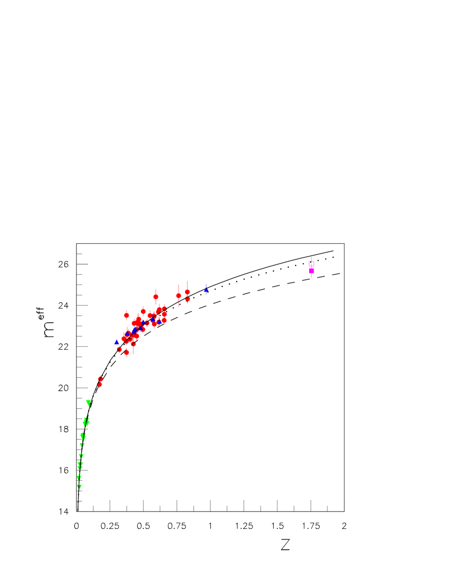
Figure 2: Hubble diagram for Type Ia supernovae data. The meaning of symbols is as follows. Calan/Tololo supernovae (full triangles down), Supernova Cosmology Project high-redshift supernovae (full circles), High-Z Supernova search Team supernovae ( full triangles up), SN 1997ff (full square) and SN 1997ff after correction for lensing (open square). Full line corresponds to the standard model $\Omega_{m}=0.3$, $\Omega_{\Lambda}=0.7$ and $\Omega_{w}=0$, dashed line to $\Omega_{m0}=0.3$, $\Omega_{\Lambda 0}=0.0$ , $\Omega_{w}=0.7$, dotted line to $\Omega_{m0}=0.3$, $\Omega_{\Lambda 0}=0.6$ , $\Omega_{w}=0.1$.

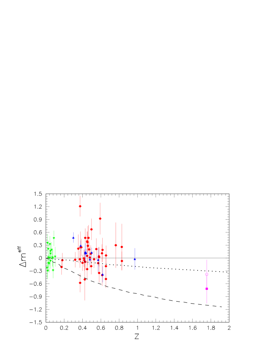
Figure 3: The magnitude residuals between data and models $\Omega_{m0}=0.3$, $\Omega_{\Lambda 0}=0.0$ , $\Omega_{w}=0.7$ (dashed line), $\Omega_{m0}=0.3$, $\Omega_{\Lambda 0}=0.6$ , $\Omega_{w}=0.1$ (dotted line) from the standard model $\Omega_{m}=0.3$, $\Omega_{\Lambda}=0.7$ and $\Omega_{w}=0$ (full line).

where ${\cal M}=M+5\log_{10}(\mbox{Mpc}/D_{H})+25$ is the Hubble-constant-free absolute magnitude, $M$ is the absolute magnitude, and $D_{H}\equiv c/H_{0}$ is the Hubble distance.
Specializing to a flat Universe in Fig. 2 we display $m(z)$ in Eq. (5.18) as a function of the redshift $z$ for the three models. The recent SN Ia sample provides measurements of the luminosity distance out to redshift $z\sim 1.7$ (SN 1997ff). In Figure 2 we also shows the Hubble diagram of effective rest-frame B magnitude corrected for the width-luminosity relation, as a function of redshift for the 42 Supernova Cosmology Project high-redshift supernovae [22], along with the 18 Calan/Tololo low-redshift supernovae [23]. We also display the 10 High-Z Supernova search Team supernovae with $0.16\leq z\leq 0.62$ [24], and the recent SN 1997ff at $z\sim 1.7$ [25]. In the case of the farthest known supernova SN 1997ff we also report the revised value of effective rest-frame B magnitude corrected after correction for lensing [26].
Even though we do not attempt to best fit the supernova data, from Fig. 2 it is evident that the model with $\Omega_{m0}=0.3$, $\Omega_{\Lambda 0}=0.0$ , $\Omega_{w}=0.7$ is excluded. On the other hand, both the standard model and the model with $\Omega_{m0}=0.3$, $\Omega_{\Lambda 0}=0.6$ , $\Omega_{w}=0.1$ are consistent with the high-z supernova data. This can be better appreciated from Fig. 3 where we display the difference between data and the fiducial standard model $\Omega_{m0}=0.3$, $\Omega_{\Lambda 0}=0.7$, $\Omega_{w}=0.0$. Thus we see that recent high-z supernova data allow that a small, but cosmological important, part of our Universe consists of an almost ideal gas of ferromagnetic domain walls.

6. CMBR constraints

As discussed in Section I, in general we expect that a network of domain wall extending over cosmological distance could lead to severe distortions of the Cosmic Microwave Background Radiation. Thus, it is important to investigate the influence of the cosmological gas of massive ferromagnetic domain walls on the Cosmic Microwave Background Radiation. If domain walls are present we have an additional temperature anisotropy:

$$\frac{\delta T}{\langle T\rangle}\;=\;\Delta\Phi\;,$$ (6.1)

where $\Phi(r)$ is the Newtonian potential of the wall network. To evaluate the temperature anisotropy Eq. (6.1) we follow the analysis performed in Ref. [27]. We find

$$\frac{\delta T}{\langle T\rangle}\;=\;\Phi(\langle L\rangle)\,n^{\nu}\;,$$ (6.2)

where $\langle L\rangle$ is the average distance between walls and $n$ is the number of walls per horizon. As concern the exponent $\nu$, it turns out that this exponent depends on the network walls configuration. According to Ref. [27] we consider values of $\nu$ between $\nu\,=\,1$ (regular network) and $\nu\,=\,3/2$ (non-evolving network). In our case, the Newtonian gravitational potential for a FDW in the $(x,y)$ plane is $\phi(z)=4\pi G_{N}|z|\sigma_{w}$ . Moreover we have $n=d_{H}/\langle L\rangle$, so that from Eq. (4.2) we obtain:

$$\frac{\delta T}{\langle T\rangle}=4\,\pi\,G_{N}\,\sigma_{w}^{2-\nu}\gamma^{2(1-\nu)}\,d_{H}^{\nu}\,\Omega_{w}^{\nu-1}\,\rho_{c}^{\nu-1}.$$ (6.3)

The quantities in Eq. (6.3) need to be evaluated at the present time $t_{0}$. Let us observe that:

$$d_{H}(t_{0})=R(t_{0})\int^{t_{0}}_{0}\!\!\frac{dt}{R(t)}=t_{0}\int^{1}_{0}\!\!\frac{d\tau}{r(\tau)}\,,$$ (6.4)

where $r(\tau)=R(t)/R(t_{0})$, $\tau=t/t_{0}$, and

$$\sigma_{w}(t_{0})=\sigma_{w}(t_{ew})\left(\frac{R(t_{ew})}{R(t_{0})}\right)^{\!\!3}=\sigma_{w}(t_{ew})\,r_{ew}^{3}\,,$$ (6.5)

$t_{ew}$ denoting the time at the electroweak phase transition.
Now, we recall that $r(\tau)$ is solution of the equation:

$$\frac{dr(\tau)}{d\tau}=t_{0}H_{0}\,\left[\Omega_{m0}r^{-1}+\Omega_{w0}r^{-2}+\Omega_{\Lambda 0}r^{2}\right]^{1/2}.$$ (6.6)

Putting $f(r)=(\Omega_{m0}r^{-1}+\Omega_{w0}r^{-2}+\Omega_{\Lambda 0}r^{2})^{1/2}$ we have

$$t_{0}=H_{0}^{-1}\int_{0}^{1}\!\!\frac{dr}{f(r)}\,.$$ (6.7)

So that we can write:

$$\frac{\delta T}{\langle T\rangle}=\alpha_{\nu}\,[\,G_{N}\,\sigma_{w}(t_{ew})\,t_{ew}^{3/2}\,H_{0}^{1/2}\,]^{\,2-\nu},$$ (6.8)

where

$$\alpha_{\nu}=\frac{256}{3}\pi^{2}\left(\frac{3\sqrt{2}}{32\pi}\right)^{\!\nu}\gamma^{2(1-\nu)}\,\Omega_{w}^{\frac{\nu+2}{4}}\left(\int_{0}^{1}\!\!\frac{dx}{r(x)}\,\int_{0}^{1}\!\!\frac{dx}{f(x)}\right)^{\!\nu}\!\!.$$ (6.9)

Eqs. (6.8,6.9) give an approximate estimate of $\,\delta T/\langle T\rangle$.
Taking $G_{N}\,\sim(10^{19}\,\text{GeV})^{-2}$, $\sigma_{w}(t_{ew})\,\sim\,10^{6}\,\text{GeV}^{3}$, $t_{ew}\,\sim\,10^{13}\,\text{GeV}^{-1}$, $H_{0}\,\sim\,10^{-42}\text{ GeV}$ [17], and assuming $\Omega_{m}=0.3$, $\Omega_{w}=0.1$, $\Omega_{\Lambda}=0.6$, we obtain:

$$\frac{\delta T}{\langle T\rangle}\!\! \sim \!\!10^{-33}\;\;\;\;\text{for}\,\,\,\nu=1\,,$$ (6.10)

$$\frac{\delta T}{\langle T\rangle}\!\! \sim \!\!10^{-17}\;\gamma^{-1}\;\;\;\;\text{for}\,\,\,\nu=3/2\,.$$

Even in the worst case $\nu\,=\,3/2$ the contributions to the large-scale anisotropy of the microwave background radiation is completely negligible given the observed value $\delta T/T\sim 10^{-6}$ [19, 20, 21].

7. Conclusions

Let us conclude by stressing the main results of the paper. From the constraint that domain walls must not destroy the observed isotropy of the Universe, it is widely believed that domain walls that might have been produced in the standard particle physics phase transitions in the very early Universe have been eliminated by some mechanism. We have discussed a new mechanism which allows domain walls produced during the primordial electroweak phase transition. Indeed, the effective surface tension of these domain walls can be made vanishingly small due to a peculiar magnetic condensation induced by fermion zero modes localized on the wall. As a consequence, the domain wall acquires a non zero magnetic field perpendicular to the wall, and it becomes almost invisible as far as gravitational effects are concerned. We find that in the perfect gas approximation the domain wall network behaves like a radiation gas. The analysis of the recent high-redshift supernova data suggests that a small component of our Universe could be composed of this gas of ferromagnetic domain walls. Finally, we showed that ferromagnetic domain wall gas induces a completely negligible contribution to the large-scale anisotropy of the microwave background radiation.

Undoubtedly, the presence of a network of massive FDWs can have influenced physical processes that took place in the early Universe. It should keep in mind that in studying effects occurred in the early Universe (say before or during the formation of large scale structures) the perfect gas approximation in no longer valid and a more complicated analysis of the interaction of walls with the primordial plasma must be in order. We reserve such subject matter to future investigations.

Appendix A Appendix

We are interested in the Dirac equation with a kink wall and in presence of the electromagnetic field $A_{\mu}(x)$:

$$(i\,/\!\!\!\partial-e\;/\!\!\!\!\!\>\!A-g_{Y}\,\phi)\,\psi=0\;.$$ (A.1)

To solve Eq. (A.1) we assume that

$$\psi=(i\,/\!\!\!\partial-e\;/\!\!\!\!\!\>\!A+g_{Y}\,\phi)\,\Phi.$$ (A.2)

Inserting Eq.(A.2) into Eq. (A.1) we readily obtain:

$$(-\partial^{2}-2ieA_{\mu}\partial^{\mu}+e^{2}A^{2}-\xi^{2}g^{2}+i\xi\,/\!\!\!\partial g-\frac{e}{2}\sigma^{\mu\nu}F_{\mu\nu})\,\Phi=0,$$ (A.3)

with $\xi=g_{Y}\,v$, $g(z)=\tanh(z/\Delta)$. It is easy to see that the solution of Eq. (A.3) factorize as:

$$\Phi(x,y,z,t)=f(x,y)\,\chi(z,t),$$ (A.4)

where $f$ is a scalar function which describes the motion transverse to the wall and $\chi$ is the spinorial part of the wave function of fermions localized on the wall. Putting $\chi(z,t)=e^{-iEt}\,\chi(z)$ we get for $f$ and $\chi$:

$$(\partial_{x}^{2}+\partial_{y}^{2}-2ieBx\partial_{y}-e^{2}B^{2}x^{2}+\beta)\,f(x,y)=0,$$ (A.5)

$$(\partial_{z}^{2}+i\xi\gamma^{3}\partial_{z}g-\xi^{2}g^{2}+ieB\gamma^{1}\gamma^{2}+\alpha)\,\chi(z)=0,$$ (A.6)

where $\alpha$ and $\beta$ are constants subject to following relation:

$$E^{2}=\alpha+\beta.$$ (A.7)

The solution of Eq. (A.5) is:

$$f_{n,p}(x,y)=A_{n}\,e^{-\frac{1}{2}\zeta^{2}\,+\,ipy}\,H_{n}(\zeta),$$ (A.8)

where

$$A_{n}=\frac{\pi^{-1/4}}{\sqrt{2^{n}n!}}\,,\;\;\;\;\zeta=\sqrt{|e|B}\left(x-\frac{p}{eB}\right),$$ (A.9)

$H_{n}(x)$ are Hermite polynomials and

$$\beta=|e|B(2n+1),\;\;\;\;\;n=0,1,2,...$$ (A.10)

In order to solve Eq. (A.6), we expand $\chi(z)$ in terms of spinors $u_{\pm}^{1,2}$ eingenstates of $\gamma^{3}$

$$\chi(z)=\phi_{\pm}^{1,2}u_{\pm}^{1,2}.$$ (A.11)

Using the standard representation for the Dirac matrices [28] we find:

$$u_{\pm}^{1}=\left(\begin{array}[]{c}1\\ 0\\ \pm i\\ 0\end{array}\right)\!,\;\;\;\;\;u_{\pm}^{2}=\left(\begin{array}[]{c}0\\ 1\\ 0\\ \mp i\end{array}\right)\!.$$ (A.12)

It is straightforward to check that:

$$\gamma^{0}u_{\pm}^{1,2}\!\! = \!\!u_{\mp}^{1,2},$$ (A.13)

$$\gamma^{1}u_{\pm}^{1}\!\! = \!\!\pm iu_{\mp}^{2}\,,$$

$$\gamma^{1}u_{\pm}^{2}\!\! = \!\!\mp iu_{\mp}^{1}\,,$$

$$\gamma^{2}u_{\pm}^{1,2}\!\! = \!\!\mp u_{\mp}^{2,1},$$

$$\gamma^{3}u_{\pm}^{1,2}\!\! = \!\!\pm iu_{\pm}^{1,2}.$$

Taking into account Eqs. (A.6), (A.11) and (A.13) we obtain:

$$(\partial_{z}^{2}\mp\xi\partial_{z}g-\xi^{2}g^{2}+eB+\alpha)\,\phi_{\pm}^{1}(z)=0,$$ (A.14)

$$(\partial_{z}^{2}\mp\xi\partial_{z}g-\xi^{2}g^{2}-eB+\alpha)\,\phi_{\pm}^{2}(z)=0.$$ (A.15)

It easy to see that there are localized states if

$$\alpha\!\! = \!\!-eB\;\;\;\;\mbox{for}\;\;\phi_{\pm}^{1},$$ (A.16)

$$\alpha\!\! = \!\!+eB\;\;\;\;\mbox{for}\;\;\phi_{\pm}^{2}.$$ (A.17)

Inserting Eqs. (A.10), (A.16), (A.17) into Eq. (A.7) we get the energy spectrum for localized states:

$$E_{n}=\sqrt{2n|e|B}\;\;\;\;\;n=1,2,...$$ (A.18)

We can now solve Eqs. (A.14) and (A.15) whit the constrains (A.16) and (A.17); we find:

$$\phi_{\pm}^{1,2}(z)=N\,\exp{\left(\pm\,\xi\int_{0}^{z}\!dz^{\prime}g(z^{\prime})\right)},$$ (A.19)

where the normalization constant $N$ is evaluated below. The solutions $\phi_{+}^{1,2}$ do not correspond to localized states and will be discarded. Inserting Eqs. (A.19), (A.11), (A.8), and (A.4) into Eq. (A.2) it easy to recover our Eqs. (3.2)-(3.5). Finally, the normalization constant $N$ can be obtained by imposing the normalization conditions:

$$\int{\!d^{3}x\,\psi^{\dagger}_{n,p,s}({\bf x})\,\psi_{n^{\prime},p^{\prime},s^{\prime}}({\bf x})}=\delta_{nn^{\prime}}\,\delta_{ss^{\prime}}\,\delta(p-p^{\prime})\;.$$ (A.20)

It is straightforward to obtain:

$$N^{2}=\frac{\sqrt{|e|B}}{8\pi\Delta\mbox{B}(\xi\Delta,1/2)\,E^{2}}\,\;.$$ (A.21)

Figure 1: Evolution of expansion parameter for three different models.

References

- [1] A. Vilenkin and E. P. S. Shellard, Cosmic Strings and Other Topological Defects (Cambridge University Press, Cambridge, 1994).
- [2] T. W. B. Kibble, J. Phys. A9 (1976) 1387.
- [3] T. W. B. Kibble, Phys. Rept. 67 (1980) 183.
- [4] W. H. Zurek, Nature 317 (1985) 505.
- [5] W. H. Zurek, Phys. Rept. 276 (1996) 177.
- [6] K. Kajantie, M. Laine, K. Rummukainen, and M. E. Shaposhnikov, Phys. Rev. Lett. 77 (1996) 2887.
- [7] F. Csikor, Z. Fodor and J. Heitger, Phys. Rev. Lett. 82 (1999) 21; Z. Fodor, Nucl. Phys. Proc. Suppl. 83 (2000) 121.
- [8] Y. B. Zeldovich, I. Y. Kobzarev, and L. B. Okun, Zh. Eksp. Teor. Fiz. 67 (1974) 3.
- [9] P. Cea and L. Tedesco, Phys. Lett. B450 (1999) 61.
- [10] P. Cea and L. Tedesco, J. Phys. G26 (2000) 411.
- [11] T. Vachaspati, Phys. Lett. B265 (1991) 258.
- [12] P. Cea, Phys. Rev. D32 (1985) 2785; D34 (1986) 3229.
- [13] A. D. Dolgov, Generation of magnetic fields in Cosmology, hep-ph/0110293.
- [14] P. Cea and L. Tedesco, Int. J. Mod. Phys. D 12 (2003) 663.
- [15] L. Campanelli, P. Cea, G. L. Fogli, L. Tedesco, Phys. Rev. D65 (2002) 085004.
- [16] A.Ayala, J.Jalilian-Marian, L.D. McLerran and A.P.Visher, Phys Rev. D49 (1994) 5559; A.Ayala, J.Besprosvany, G.Pallares and G. Piccinelli, Phys. Rev. D64 (2001) 123529; A.Ayala, G.Piccinelli, G. Pallares, Phys. Rev. D66 (2002) 103503; A.Ayala, J. Besprosvany, Nucl. Phys. B651 (2003) 211.
- [17] E. W. Kolb and M. S. Turner, The Early Universe (Addison-Wesley, Redwood City, California, 1990).
- [18] L. Campanelli, P. Cea, G. L. Fogli and L. Tedesco, arXiv:astro-ph/0304524, International Journal of Modern Physics D to appear.
- [19] A. Balbi et al., Astrophys. J. 545 (2000) L1 [Erratum-ibid. 558 (2001) L145] [arXiv:astro-ph/0005124].
- [20] P. de Bernardis et al., Astrophys. J. 564 (2002) 559 [arXiv:astro-ph/0105296].
- [21] C. L. Bennett et al., arXiv:astro-ph/0302207.
- [22] S. Perlmutter et al. [Supernova Cosmology Project Collaboration], Astrophys. J. 517 (1999) 565.
- [23] M. Hamuy et al., Astrophys. J. 112 (1996) 2391.
- [24] A. G. Riess et al., Astrophys. J. 116 (1998) 1009.
- [25] A. G. Riess et al., Astrophys. J. 560 (2001) 49.
- [26] N. Benitez, A. G. Riess, P. E. Nugent, M. Dickinson, R. Chornock and A. V. Filippenko, Astrophys. J. 577 (2002) L1.
- [27] A. Friedland, H. Murayama and M. Perelstein, Phys. Rev. D 67 (2003) 043519 [arXiv:astro-ph/0205520].
- [28] J. D. Bjorken and S. Drell, Relativistic Quantum Fields (McGraw Hill, New York, 1962).