Scale-Free Magnetic Networks: Comparing Observational Data with a Self-Organizing Model of the Coronal Field

Abstract

We propose that the coronal magnetic field, linking concentrations on the photosphere through an interwoven web of flux, embodies a scale-free network. It arises from a self-organized critical dynamics including flux emergence, the diffusion and merging of magnetic concentrations, as well as avalanches of reconnecting flux tubes. Magnetic concentrations such as fragments, pores and sunspots, are ‘nodes’ joined by flux tubes or ‘links’. The number of links emanating from a node is scale-free. We reanalyze the quiet-Sun data of Close et al and show that the distribution of magnetic concentration strengths is a power law with an index $\gamma=1.7\pm 0.3$, over the entire range of the measurement, about $(2-500)\times 10^{17}$ Mx. This distribution is compatible with that for the sizes of active regions reported by Harvey and Schwaan. Thus magnetic concentrations may be scale-free from the smallest measurable fragments to the large active regions. Numerical simulations of a self-organized critical model give the same index $\gamma$, within statistical uncertainty. The exponential distribution of flux tube lengths also agrees quantitatively with results from the model, below the supergranule cell size. Calibration with the measured diffusion constant of magnetic concentrations allows us to calculate a flux turnover time in the model to be of order 10 hours and the total solar flux to be of order $10^{23}$Mx, agreeing with observations. We introduce two other statistical quantities to characterize scale-free networks. The probability distribution for the amount of flux connecting a pair of concentrations, and the number of distinct concentrations linked to a given one are predicted to be scale-free, with different indices. Our approach unifies the observation of scale free flare energies with the coronal magnetic field structure.

1 Introduction

A complex interwoven network of magnetic fields threads the surface of the sun. Magnetic energy stored in the coronal network builds up due to turbulent plasma forces below the photosphere until stresses are suddenly released by reconnection (Priest & Forbes 2000; Parker 1994). If the magnetic energy released is sufficiently large, it induces radiative emission that is detected as a flare event. Flares are often classified into hard X-ray flares, EUV transient brightenings, nanoflares, etc. However, observations show that one cannot associate any length, time, or energy scale to flares overall. In particular, the probability distribution of flare energies appears as a featureless power law that spans more than eight orders of magnitude, which is the entire observable range (Aschwanden et al. 2000). This points to a scale-invariant energy release mechanism. Lu & Hamilton (1991) first proposed that the corona is in a self-organized critical (SOC) state, with avalanches of all sizes (Bak et al. 1987). In this picture, all flares large and small, come from avalanches of magnetic reconnection. SOC systems often show scale free behavior not only for their event statistics but also for emergent spatial and temporal structures, as seen both in physical systems (e.g. Frette et al. (1996)) and numerical models (e.g. Hughes & Paczuski (2002)). For a review see Bak (1996).

Like flares, concentrations of magnetic flux on the photosphere also exist on a wide variety of scales. The strongest concentrations are sunspots, which occur in active regions that may contain more than $10^{22}$Mx, at smaller scales are ephemeral regions, pores and, at the smallest resolvable concentrations above the current resolution scale of $\approx 10^{16}$Mx, are fragments. The structure of the quiet-Sun has been described as a ‘magnetic carpet’ with magnetic concentrations of various strengths linked by flux tubes (Schrijver et al. 1997).

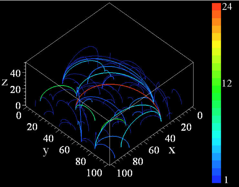
Together with Dendy, Helander, and McClements, we recently introduced a multi-loop model of the coronal magnetic field that exhibits self-organized criticality (Hughes et al. 2003). Photospheric magnetic flux concentrations, represented by points on a surface, are connected by loops, representing flux tubes. The model exhibits reconnection avalanches of all sizes, and thus a power law distribution of flare events. The structure of the magnetic network in the model qualitatively resembles the magnetic carpet, as shown in Figure 1. Its structure is mathematically described as a scale-free network (Barabasi & Albert 1999). The model provides a single physical process which gives rise to both a scale free magnetic field structure as well as a power law distribution of flares. Thus flare event statistics are unified with the scale free geometry of the coronal magnetic field.

Figure 1: Snapshot of loops in the steady state of the model. Footpoints lie in the $(xy)$ plane and are linked by loops. The loops are colored to indicate the relative strength of the connection, as shown by the scale to the right. Note that there is a large range in the number of loops emanating from different footpoints, as well as a wide range of connection strengths. The figure was generated with model I using parameters $L=100$, $m=1$.

Here, we make a detailed study of the properties of the network. This provides a quantitative basis enabling direct statistical comparison between the network structure of the coronal magnetic field and of the model. To this end, we reanalyze recent measurements of the distribution of strengths of magnetic flux from Close et al. (2003) and Hagenaar et al. (2003). We find that the strength of magnetic flux concentrations are scale-free, as predicted by the model.

Based on this quantitative statistical comparison, we propose that the coronal magnetic field embodies a scale-free network that emerges as a consequence of a SOC dynamics involving avalanches of reconnection. Magnetic concentrations on the photosphere are nodes in the network while flux tubes are links connecting the nodes. The defining signature of a scale-free network is that the number of links attached to any node is distributed according to a power law. Physically, this means that the amount of flux emanating from a magnetic concentration on the photosphere is scale-invariant up to a cutoff determined by the overall system size – in this case the total amount of flux emanating from the photosphere.

Scale-free networks arise in many different contexts, including the internet (Faloustos et al. 1999), the World Wide Web (Barabasi & Albert 1999), interaction and regulatory networks (Wagner 2001; Maslov & Sneppen 2002), or the citation network (Redner 1998), for a review see e.g. Albert & Barabási (2002); Bornholdt & Schuster (2002). There is currently an extensive research effort to study the consequences of that observation in biological and social phenomena. Unlike previous models, in our model the network itself emerges as a consequence of the dynamics, and is not, a priori, forced or assumed to exist as a system-wide network.

Section 2 gives a general explanation of the model and then a detailed definition. The latter may be skipped by readers primarily interested in the results. Section 3 contains a quantitative comparison between numerical simulation results and reanalyzed observational data for the distribution of magnetic concentration strengths. A single calibration is used, setting the loop unit in the model equal to the minimum magnetic flux threshold that can currently be detected. The connection with scale-free networks is established. In Section 4 we compare the exponential distribution of flux tube lengths in the model with observational data of Close et al; this allows a calibration of the length unit in the model to distances on the photosphere. This length scale calibration allows a further calibration of the time unit of the model by using measurements of the diffusion constant of magnetic concentrations (Hagenaar et al. 1999). We thereby calculate the flux emergence and turnover rate predicted by the model, and compare with current estimates for the solar magnetic field. We also propose new statistical quantities that can be measured to quantify the statistical properties of the coronal network structure, and make predictions for them. These are the distribution of the flux strengths between pairs of opposite polarity concentrations, and the distribution of the number of distinct concentrations connected to any given one. These describe a network where typical magnetic concentrations are connected to many other ones, but most of the flux emanating from one concentration is typically linked to only one other concentration. The main results and conclusions are summarized in section 5.

2 The SOC Model

The coronal magnetic field consists of magnetic flux concentrations on the photosphere linked by magnetic fields, or flux tubes. Five processes have been identified for the quiet-Sun: (i) emergence - magnetic flux tubes are injected from beneath the photosphere, or may be removed (submergence); (ii) diffusion - the footpoints of the flux tubes are continuously agitated by the turbulent convection of the plasma; (iii) coalescence - footpoints of the same sign merge to form concentrations and these concentrations can aggregate to form even larger concentrations; (iv) cancellation - mutual loss of flux from opposite polarity concentrations; (v) fragmentation - the break up of concentrations into smaller ones.

All these processes refer explicitly to dynamics that can be observed in magnetic images of the photosphere. To this we add another process, (vi) reconnection - flux tubes linking the concentrations reconnect in the corona when magnetic field gradients become sufficiently steep. Reconnection of flux tubes lowers the magnetic field energy but, by itself, does not alter strength of the concentrations. Currently, the model does not include an explicit fragmentation process.

2.1 Explanation of the Model

Although it may seem unwieldy, it is actually straightforward to construct a physically motivated model where these processes are unavoidably realized. Of course, in order to describe magnetic field evolution both at large energy and length scales, and at the extremely high magnetic Reynolds number relevant to the corona, it is necessary to make simplifications of the underlying physical laws. Nevertheless, the model does retain certain physical features that are known to be important. Primarily, it keeps track of the geometrical constraints that the high conductivity of the corona and the physics of reconnection impose on magnetic field evolution. Magnetic flux is frozen into the plasma and is constrained to move with it. However, when magnetic field gradients are steep reconnection can occur, changing the geometry of the magnetic field structure. Secondly, diffusion of footpoints and flux emergence are considered to be the dominant sources driving coronal magnetic field energy.

The fundamental entity in the model is a directed loop which traces the midline of a flux tube and is anchored to a surface at two opposite polarity footpoints. A collection of these loops and their footpoints gives a representation of a coronal magnetic field structure. It is able to describe fields that are very complicated or interwoven, like the magnetic carpet. A snapshot of a configuration in the steady-state is shown in Fig. 1. The number of loops connecting any pair of footpoints is indicated by a color-coding. It is evident that both the number of loops attached to a footpoint and the strength of those loops vary over a broad range.

Loops injected at small length scales are stretched and shrunk as their footpoints diffuse over the surface. Loops submerge when their footpoints approach closely. Nearby footpoints of the same polarity coalesce, to form magnetic fragments, which can themselves coalesce to form ever larger concentrations of flux, such as pores and sunspots. Conversely, opposite polarity footpoints may cancel (though see section 2.3). Loops can reconnect when they collide in three dimensional space, thereby releasing magnetic energy. Reconnection of flux tubes or concentration cancelation may trigger a cascade of further reconnection, representing a flare.

2.2 Definition of the Model

1.  Flux Tube: Each flux tube is represented by an infinitesimally thin, directed loop which traces its midline. A coronal magnetic field is described by a configuration of many of these loops. For simplicity each loop is considered to be a semicircle emerging perpendicular to the $(xy)$ plane. Every loop has a positive footpoint, where magnetic flux emerges from the photosphere, and a negative one, where flux returns. The size of the system in the $(xy)$ plane, which represents a region of the photospheric surface, is $L\times L$. Loops are labeled by an integer, $n$, and the positions of the two footpoints of the $n$th loop are labeled in the $(xy)$ plane by ${\bf r}^{+}_{n}$ and ${\bf r}^{-}_{n}$. The footpoint separation of a flux tube is then $d_{n}=|{\bf r}^{+}_{n}-{\bf r}^{-}_{n}|$ and the length of a flux tube is $l_{n}={\pi\over 2}|{\bf r}^{+}_{n}-{\bf r}^{-}_{n}|$

2.  Magnetic Concentration: A footpoint labels the center of a magnetic concentration. Due to coalescence, described in step 6, a footpoint can have more than one loop attached to it. This means that the magnetic flux from any concentration, or the flux connecting any two concentrations, can be arbitrarily large, despite the fact that the individual loops, defined in step 1 represent small, quantized units of flux. We do not attach a surface area to the concentrations, just as we do not attach a width to flux tubes. A concentration in the model is completely described by a single footpoint located at its center and the number of loops connected to the footpoint represents the total flux of the fragment. To compare with observations, one loop in the model should be set equal to the minimum threshold for flux to be included in the data set.

3.  Footpoint stirring: This and the next term represent the driving terms for magnetic flux. The diffusion of footpoints, and therefore the concentrations they represent, is described as a random walk on the two dimensional $(xy)$ plane. At an update step, an arbitrary footpoint is chosen at random and its position is moved, ${\bf r}\rightarrow{\bf r}+\Delta{\bf r}$. The vector $\Delta{\bf r}$ has length and angle chosen randomly from uniform distributions between 0 and $1$, and 0 and $2\pi$, respectively. If the initial loop lengths are small, footpoint diffusion will cause an average increase in the length of the loops. In this way, photospheric turbulence pumps magnetic energy into the coronal field. For simplicity, we usually study a system with open reflective boundary conditions; if a footpoint attempts to move outside the $L\times L$ box in the $(xy)$ plane, it is elastically reflected back into the box.

4.  Flux emergence and submergence: Small loops are injected into the system at random locations, with footpoints initially separated by a distance $l_{nl}=4$. Loops with footpoints closer than distance $l_{min}=2$ are removed from the system, corresponding to loop submergence. The precise (small) length scales of these two processes do not effect the large scale properties of the system. The essential feature is that at small length scales the model dynamically maintains a flow of loops. Thus the magnetic field of the corona is represented as an open system, and the flux in the system will turnover in time or be replaced with new flux.

New flux is injected at a rate determined by a control parameter $m$. This quantity is defined as follows: the number of footpoint updates (step 3) that separate an injection of flux (step 4) is $m$ times the number of footpoints in the system at that time. Thus $m$ is the average number of random walk steps a footpoint will experience between new loops injected into the system.

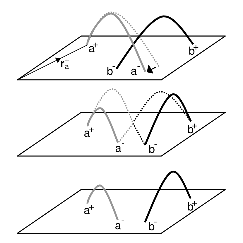
5.   Reconnection of Flux Tubes: Reconnection can occur when either (a) two loops collide in three dimensional space, or (b) two footpoints cancel or annihilate as explained in step 7. In the first case, the midlines of two flux tubes have crossed resulting in a strong magnetic field gradient at that point. The flux emerging from the positive footpoint of one of the reconnecting loops is then no longer constrained to end up at the other footpoint of the same loop, but may instead go to the negative footpoint of the other loop (see Figure 2). Reconnection is only allowed if it shortens the combined length of the two colliding loops. This process is rapid compared to all other processes because information is transmitted along the flux tubes at the Alfvén speed. It occurs instantaneously in the model.

If rewiring occurs, it may happen that one or both loops need to cross some other loop in order to reach its rewired state. Thus a single reconnection between a pair of loops can trigger a cascade of causally related reconnection events. The reconnection dynamics of multiply connected footpoints that were used in the numerical simulations is a straightforward extension (D. Hughes, in preparation).

Figure 2: Diagram showing the process of a reconnection event, from top to bottom. In frame 1 loop $a$ moves from its previous position (dashed line) and crosses loop $b$. In frame 2 the loops exchange footpoints and move to their rewired state. Frame 3 shows the final relaxed configuration.

6.   Coalescence: If a footpoint moves within the distance $l_{min}$ of another footpoint of the same polarity, it is reassigned to the latter footpoint’s position and they move as one footpoint thereafter. The two linked footpoints therefore form a single magnetic concentration whose center is located at the footpoint’s position.

7.   Cancelation: Footpoints of opposite polarity, belonging to different flux tubes, can annihilate when they approach on the photosphere (Livi et al. 1985; Priest & Forbes 2000). When footpoints of opposite polarity, belonging to different loops, approach within a distance $l_{min}$ in the model, both footpoints are eliminated and the remaining two footpoints are attached, forming one loop, where before there were two. The annihilation dynamics of concentrations with more than one attached loop can be implemented in different ways (D. Hughes, in preparation). The scaling behavior of the model does not appear to be sensitive to the precise algorithm. Footpoint annihilation may cause collisions between loops leading to further reconnection, as per step 5.

2.3 Simulations and parameters

Here we present results from numerical simulations of two different models: model I includes cancelation (step 7) and model II does not. Both models I and II include the submergence of small loops (as per step 4). Note that in Hughes et al. (2003), numerical results were presented only for model I.

For each version, the configuration of loops slowly evolves in response to the driving, coalescence and reconnection processes. It reaches a dynamic steady state whose statistical character is independent of the initial conditions. In this and the following sections, numerical simulation results are presented for a range of system sizes $L=25$ to $200$ and stirring rates $m=0.001$ to $10$, including approximately $10^{7}$ avalanches of reconnection events in the steady state, for each of the two models. The statistical behavior is robust on varying the stirring rate $m$, and system size $L$, even though the total number of loops and footpoints in the system vary widely.

3 Distribution of Magnetic Concentration Strengths

In this section, we reanalyze observational data for the distribution of magnetic concentration strengths, and compare with results from numerical simulations of the SOC model. This provides a calibration between the flux loop in the model and magnetic flux on the photosphere. The connection with scale-free networks is established.

3.1 Observational data of Close et al

Close et al. (2003) report the cumulative distribution of fragment sizes, measured in terms of their total magnetic flux, in a balanced section of the quiet-Sun. They analyzed high-resolution MDI magnetograms. The flux in a magnetogram image of the photosphere of size 88Mm$\times$88Mm was represented by a series of point sources. A macropixel contained a point source if the absolute flux density in the pixel exceeded a threshold of $1.55\times 10^{17}$Mx. Magnetic field lines corresponding to the potential field were traced between these point sources. Each field line represents the same amount of magnetic flux. Close et al argued that it is reasonable to consider the field lines as flux tubes. Loops in our model thus correspond to the field lines calculated by Close et al. Obviously, at the scale of the system size the net flux in our model is zero so we are only comparing with their balanced data.

3.1.1 A reanalysis of the data of Close et al

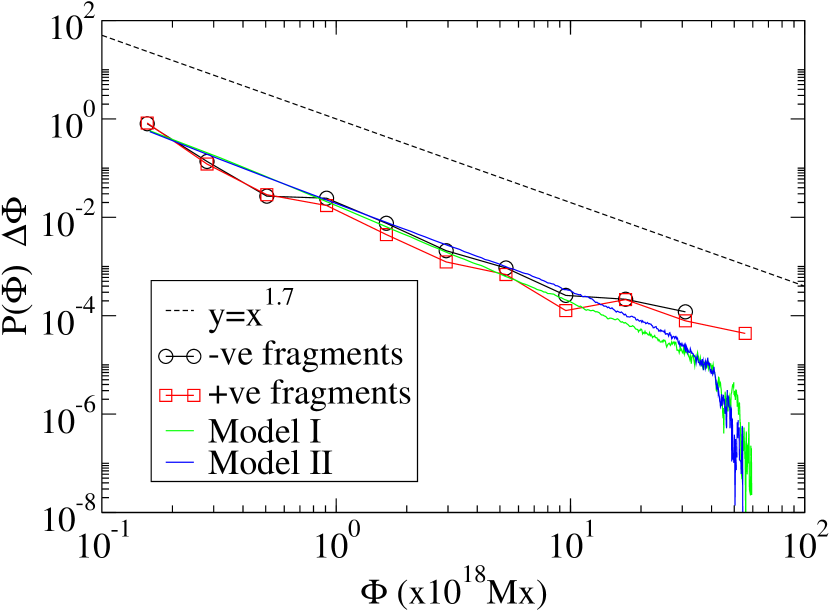
The data was originally presented using a log-linear plot, which is appropriate for distributions with one, or a few, characteristic scale(s), such as the exponential distribution. We have reanalyzed this data to determine the normalized histogram of concentration strengths, as shown in Figure 3, plotted on a double logarithmic scale.

First, the fraction of positive (negative) magnetic fragments, or concentrations, in bins of size $\Delta\Phi=1.55\times 10^{17}Mx$ were computed from the cumulative distributions reported in Figure 5 of Close et al. (2003). This value of $\Delta\Phi$ was chosen to correspond to the minimum threshold resolution reported in Close et al. For each bin, this fraction, $P(\Phi)\Delta\Phi$, is the number of concentrations in that bin divided by the total number of concentrations detected. Then we aggregated these bins into logarithmically increasing ones, and divided by the number of $\Delta\Phi$ bins in each logarithmic one. The logarithmic aggregation is done solely to increase the accuracy at larger fragment sizes.

As demonstrated in Figure 3, within statistical uncertainty, the distribution of fragment sizes is a power law both for positive and negative concentrations over the entire range of the measurement, about $(2-500)\times 10^{17}$ Mx; i.e.

$$P(\Phi)\Delta\Phi\sim\left({\Phi\over\Delta\Phi}\right)^{-\gamma}{\rm\ with\ }\gamma=1.7\pm 0.3\,.$$ (1)

This shows that magnetic concentrations form a scale free network.

Figure 3: The degree distribution of the magnetic network. The normalized number of magnetic concentrations in bins of size $\Delta\Phi=1.55\times 10^{17}$ Mx obtained by reanalyzing the measurement data originally shown in Figure 5 of Close et al. (2003). The straight line has a slope -1.7 corresponding to equation 1. The model data shown represents the probability distribution, $P(k_{foot})$, for number of loops, $k_{foot}$, connected to a footpoint. This has been rescaled so that one loop, $k_{foot}=1$, equals the minimum threshold of flux, $1.55\times 10^{17}$ Mx (see equation 2). The parameters used were $m=0.1,L=100$ for model I and $m=1,L=100$ for model II.

3.2 Model Results and Comparisons

The number of loops attached to a footpoint is an integer, $k_{foot}$, which is greater than or equal to one. The distribution $P(k_{foot})$ measures the likelihood that a footpoint selected at random will have $k_{foot}$ loops attached to it. This number corresponds to the amount of flux observed in a concentration on the photosphere, since each concentration is identified by a single footpoint locating its center. In the context of networks, the integer $k_{foot}$ is normally written simply as $k$, which is the number of links attached to a node. The quantity $k$ is referred to as the degree of the node, and $P(k)$ is referred to as the degree distribution of the network.

Figure 3 compares results from numerical simulations of models I and II with the observational data. It is necessary to calibrate units of flux in the model to actual flux on the photosphere. The integer loop unit in the model was set equal to the minimum threshold resolution used by Close et al, i.e.

$$\Phi=k_{foot}\times(1.55\times 10^{17}{\rm Mx}).$$ (2)

Otherwise, the comparison involves no fitting parameters. Over the range where concentrations were detected, agreement between the reanalyzed observational data and the model results are excellent. Equivalent to Eq. 1, the degree distribution of the scale free magnetic network is

$$P(k_{foot})\sim k_{foot}^{-\gamma}$$ (3)

where the critical exponent $\gamma$ is the slope of the curves shown in Figure 3. Note that if the minimum threshold resolution were changed, the calibration expressed in Eq. 2 would change correspondingly.

3.2.1 Universality classes

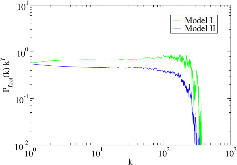
The critical exponent for models I and II are further apart than Figure 3 may suggest. For model I, $\gamma=2\pm 0.1$, whereas for model II, $\gamma=1.75\pm 0.1$. In Figure 4, we have multiplied $P(k_{foot})$ by $k_{foot}^{2}$ for model I and by $k_{foot}^{1.75}$ for model II. This tests for any systematic deviations from scaling. The resulting horizontal lines over a region spanning more than two decades provides a strong indication that the numerical simulation results are probing an asymptotic scale-free network. As the exponent $\gamma$ differs between model I and II, concentration cancelation on the surface of the photosphere appears to change the universality class of the scale-free magnetic network.

Figure 4: Scale free network exponent. The probability distribution, $P(k_{foot})$, for number of loops, $k_{foot}$, connected to a footpoint, multiplied by $k_{foot}^{\gamma}$. Models I and II require different values of gamma in order to obtain a horizontal line over the central scaling region. In this figure we use the values $\gamma=2.0$ for model I, and $\gamma=1.75$ for model II.

3.2.2 The range of scaling

Note that the cutoff in the degree distributions shown in Figure 3 and 4 is a finite size effect. With respect to the numerical simulation results, the range of scaling can be increased by e.g. increasing the system size ratio $L/l_{min}$. This allows more footpoints and loops into the system. Since the number of loops attached to any footpoint cannot exceed the total number of loops in the system, increasing $L/l_{min}$ extend the scaling range.

With respect to the observational data, the range of scaling can be extended at both the low and high flux ends. Longer observation time would make it more likely to observe large flux concentrations, which occur with relatively low probability, extending the scaling regime to higher flux strengths. A finer flux resolution would allow smaller flux concentrations to be detected, extending the range at low flux strengths.

3.3 Previous Empirical Results

Measurements of the distribution of magnetic concentrations on the quiet-Sun have been made by several groups. Schrijver et al. (1997) analyzed high resolution magnetograms from the MDI instrument on SoHO. They applied a number of filtering and selection techniques to identify ephemeral regions. They found an approximately exponential distribution of magnetic concentration strengths between about $10^{18}$ and about $5\times 10^{18}$ Mx, with a raised tail above that range. They also proposed a model, incorporating flux emergence, merging, cancelation and fragmentation, which has an exponential distribution within a certain range. Hagenaar (2001) also reported an exponential distribution in the range $(3-8.5)\times 10^{18}$ Mx.

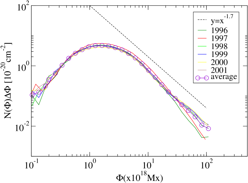
Further observations were made by Hagenaar et al. (2003). Data was obtained for different years, from 1996 to 2001 corresponding to roughly half a solar cycle. They found that the distributions of magnetic concentration sizes measured at different points in the solar cycle could be more accurately described by a sum of two exponentials over the range $(3-100)\times 10^{18}$ Mx. Their data analysis used a different algorithm to define concentrations than used by Close et al, including smoothing the magnetogram data by convolution with a Gaussian and the imposition of a filter to remove active regions.

3.3.1 A reanalysis of Hagenaar et al data

In Figure 5, the observation data from Figure 5 of Hagenaar et al. (2003) has been replotted on a double logarithmic scale. As shown, all six data sets, representing different phases of the solar cycle, are consistent with a power law tail. The figure displays the magnetic concentration counts for each year, along with an average over all six data sets. The different years follow the same curve almost exactly below $\sim 30\times 10^{18}$Mx, but differ somewhat above this value. A likely explanation is statistical noise, although it is not possible to rule out a systematic variation with the solar cycle.

It is evident that our model describes the data obtained by Close et al better than the data obtained by Hagenaar et al. This is particularly apparent at small concentration sizes. However, the roll-over at small concentrations seen in Figure 5 may be an artifact of the smoothing algorithm used in the data acquisition procedure used by Hagenaar et al and not by Close et al. In fact, a roll-over is also found in numerical simulations of our model by imposing a finite resolution grid, as described later.

Figure 5: Replotted distribution of magnetic flux measured by Hagenaar et al. (2003). Above $\sim 4\times 10^{18}$Mx the distribution is well approximated by a power law with exponent $\sim-1.7$. The roll-over at small flux values may be due to the data acquisition procedure, and is not evident in the reanalyzed data from Close et al. (2003) shown in Figure 3.

3.3.2 Active Regions

Considering larger concentrations of magnetic flux, Harvey & Zwaan (1993) report the distribution of active region areas. The observed counts can be described as an approximate power law with an index, $\gamma\simeq 2$, from about three square degrees to about forty square degrees. This index is very close to the index shown in Figure 3, for smaller magnetic concentrations on the quiet-Sun. Thus there is some empirical evidence to support our conjecture that the distribution of flux concentrations is scale invariant over a range spanning the smallest (currently) measurable concentrations to the large active regions. In other words, there is one power law for the distribution of all flux concentrations regardless of their strength, up to a cut-off set by the size of the Sun.

In numerical simulations of our model, unsurprisingly, the largest avalanches of reconnection emanate from flux tubes attached to the largest concentrations. The big concentrations could therefore be referred to as ‘sunspots’ or large opposite polarity pairs referred to as ‘active regions’. However, it is generally believed that active regions have a different origin and dynamics than smaller concentrations on the quiet-Sun. There are correlations in the dynamics of flux emergence which are not included in our model. Such correlation, if they were characterized and quantified, could be incorporated into the driving term(s) - e.g. steps 3 and 4.

3.4 Net Signed Flux in Grid Cells

The scaling behavior of critical systems is robust to coarse-graining. In fact, this is the fundamental concept behind the renormalization group, and scale invariance in general. This means that the system displays the same statistical behavior regardless of the scale of observation. Finite instrument resolution does not alter the critical properties, but only the range of observable scaling behavior. Such measurement imprecision is typically encountered at small values, i.e. short length scales or low flux values. The effect on the distribution is only seen at these low values, usually as a flattening of the distribution near the resolution limit.

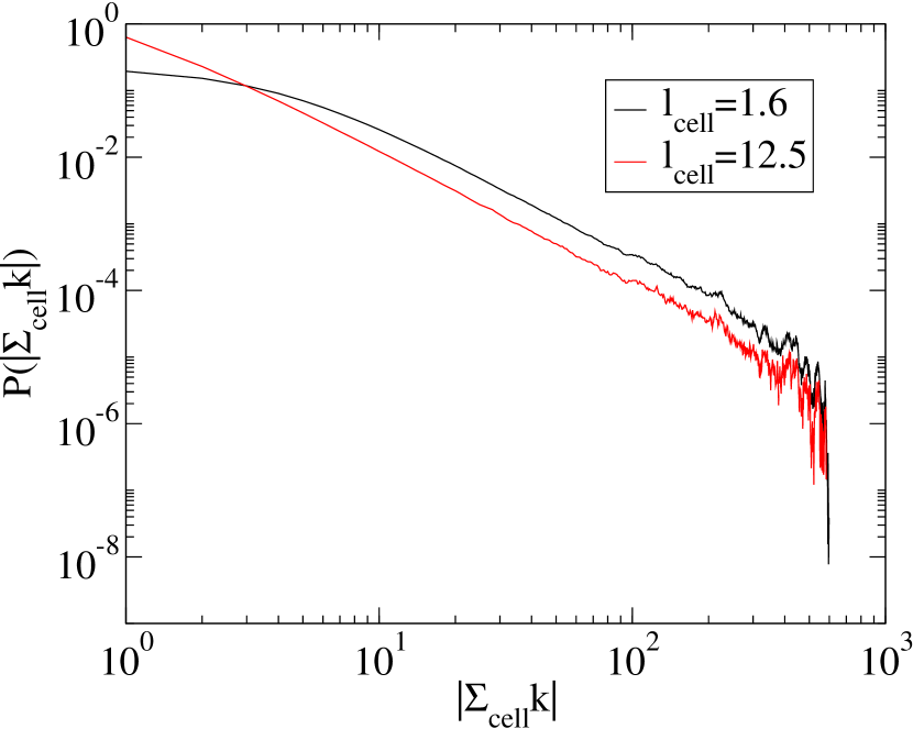
We illustrate the effect of finite resolution in the model by imposing a grid with cells of linear extent $l_{cell}$ on the system and counting the net signed flux associated with all footpoints in each cell. Since the individual distribution of footpoint strengths has a Levy tail with an infinite variance (Eq. 3), this sum is not expected to converge to a Gaussian according to the central limit theorem. Instead, the sum is dominated by the largest instance in the sample, and converges to a Levy-stable distribution. Thus the distribution of net signed flux within a grid cell asymptotically behaves as

$$P\left(\;\left|\sum_{cell}k^{\prime}_{foot}\right|\;\right)\sim\left(\;\left|\sum_{cell}k^{\prime}_{foot}\right|\;\right)^{-\gamma}\quad,$$ (4)

where $k^{\prime}_{foot}=k_{foot}$ for positive footpoints and $k^{\prime}_{foot}=-k_{foot}$ for negative footpoints.

As shown in Figure 6, coarser resolution causes a round-off at small values of $\left(\sum_{cell}k\right)$. However, the scaling behavior of the probability distribution of net signed flux within a grid cell is a power-law with the same index as for the individual footpoints, and independent the size of the grid cell, $l_{cell}$. In the model, the cutoff at large scales occurs at the same point for all grid cell lengths. It is determined by the global system size $L/l_{min}$. This is due to the unrealistic assumption that the footpoints, or magnetic concentrations, do not occupy any physical area on the surface. Associating a physical area to the footpoints would likely cause the large scale cutoff in the distribution to depend also on $l_{cell}$. The largest footpoints could cover an area larger than an individual grid cell.

Figure 6: Net signed flux within grid cells of length $l_{cell}$ for model I, with $L=100$. This shows a simulated effect of finite resolution on measurements of concentration flux. Note that the power law is robust and only the smallest scales are affected by resolution. We suspect that allowing concentrations to occupy a finite area in the model (as on the photosphere) would cause the cutoff at large scales to move to higher values with increasing $l_{cell}$.

3.4.1 A Grid Measurement

The observation of robust power law behavior, independent of the grid cell size over a range of scales, suggests a measurement of photospheric magnetic flux that does not require the identification or selection of concentrations. Nor does it require filtering images to remove active regions or any other features. An unbiased measurement for the sun, corresponding to that described here for the model, would involve imposing a mathematical grid with grid cell length of a specified size $l_{cell}$, on magnetometer images of the photosphere. The net signed magnetic flux in each grid cell $|\Phi_{cell}|$ is calculated by summing all the signed values of flux $\phi$ in pixels within the grid cell, therefore

$$\left|\Phi_{cell}\right|=\left|\sum_{cell}\phi\right|.$$ (5)

A large statistical sample could be obtained by collecting magnetometer images at different times. For each $l_{cell}$, this allows a computation of the probability distribution of net signed flux, $P(|\Phi_{cell}|)$. The model results indicate that this would yield a power law distribution of flux concentrations

$$P(|\Phi_{cell}|)\Delta\Phi\sim{\left(|\Phi_{cell}|\over{\Delta\Phi}\right)}^{-\gamma},$$ (6)

for a range of $l_{cell}$.

The cutoffs at both small and large values of flux may depend on $l_{cell}$. If the cutoff at large scales increases with $l_{cell}$, data collapse methods could be used to rescale the flux according to the cell size, so that all the distributions would coincide on the rescaled plot. We expect a similar behavior to obtain by neglecting the sign of the flux, i.e. the probability distribution for net unsigned flux within a grid cell, $P(\sum_{cell}|\phi|)$, may also be scale-free.

4 The Flux Network

The magnetic concentrations themselves do not comprise a network. They must be joined by magnetic fields, or flux tubes, in order to do so. In fact Close et al. (2003) also measured statistical properties of the magnetic flux network in the quiet-Sun that allow comparisons with our model. They found that (1) for any concentration strength there are a wide range of possible connections; (2) concentrations show a preference towards connecting to nearby opposite polarity concentrations; (3) despite the vast number of possible connections, the bulk of the flux is often divided so that most of it goes to one opposite polarity concentration.

Similar results are found in numerical simulations of our model. In fact, all of this behavior is explained by the existence of three different scale-free distributions. The first is the distribution of concentration sizes (node degree) as discussed previously. The second and third are new statistical quantities we introduce to characterize networks: (a) the amount of flux connecting a pair of concentrations, or the strength of the link between a pair of nodes, and (b) the number of distinct concentrations (nodes) linked to a given one. These are both found to be power laws in the model, with different indices. We also discuss the distribution of the lengths of flux tubes and compare with observations of Close et al. This allows a calibration of the length unit in the model to a physical length on the photosphere.

4.1 The strength of connections

Figure 7: The link strength distribution. The probability distribution, $P(k_{pair})$, of the number of loops, $k_{pair}$, connecting pairs of footpoints. $P(k_{pair})$ follows a power law with exponent $\alpha=2.25\pm 0.1$ for model I and $\alpha=2.0\pm 0.1$ for model II. The parameters used were $m=0.1,L=100$ for model I and $m=1,L=100$ for model II.

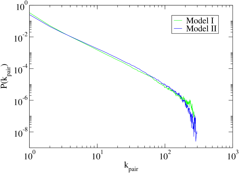
Two opposite polarity footpoints can be connected to each other by any number of loops. The number of loops connecting a pair of footpoints is defined as $k_{pair}$. This is the strength of the link between two nodes. Measuring this value over all footpoint pairs gives the distribution shown in Figure 7. Power law behavior occurs for both models, i.e.

$$P(k_{pair})\sim k_{pair}^{-\alpha}.$$ (7)

The critical index $\alpha$ is equal to $2.25\pm 0.1$ and $2\pm 0.1$ for models I and II respectively. The index $\alpha\geq\gamma$, as the number of loops connecting any pair of footpoints cannot exceed the number of loops at one of those footpoints. The cut-off at large flux values in Figure 7 is a finite size effect; increasing number of loops in the system (for example by increasing the system size) will extend the scaling region and move the cut-off to higher values. Simulation results lead us to propose that the distribution of amount of magnetic flux connecting any pair of concentrations on the photosphere is distributed as a power law, with an index $\alpha$.

4.2 The number of unique connections

One footpoint can be connected to an arbitrary number of opposite polarity footpoints. For each footpoint we count the number of distinct footpoints that are connected to it. This is $k_{unique}$. Multiple loops between a pair of footpoints are counted as a single connection in this measurement. This distribution, shown in Figure 8, may be consistent with power law behavior

$$P(k_{unique})\sim k_{unique}^{-\beta}.$$

The exponent $\beta\sim 2.8$ for model I. Since $\beta$, if it exists, is greater than 2, the average number of unique footpoints connected to any given one is finite. However, if $\beta\leq 3$ then the variance in the number of unique connections diverges.

Figure 8: The unique connection distribution, $P(k_{unique})$, for the number of unique footpoints to which a given footpoint is linked. The straight line indicates a power law with exponent $\beta\sim 2.8$. The parameters are $m=0.1$, $L=100$ for model I, and $m=1$, $L=100$ for model II.

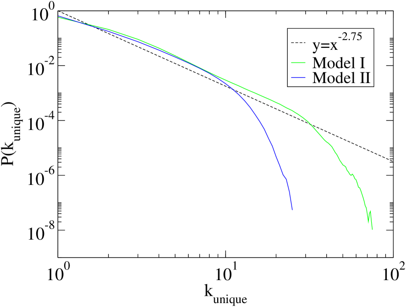
The quantities $P(k_{pair})$ and $P(k_{unique})$ are complementary measures of the network structure. The former measures the strength of connections, the latter measures the number of unique connections. Since the average number of unique connections is probably finite, concentrations with high flux values are more likely to have a small number of strong connections than a large number of weak ones. These results agree qualitatively with observations of Close et al listed at the start of section 4. It may be possible to measure the quantities $P(k_{pair})$ and $P(k_{unique})$ on the Sun.

It is not required that both $P(k_{pair})$ and $P(k_{unique})$ follow power law behavior in order to obtain a scale free network. The only requirement is that the degree distribution $P(k_{foot})$ is scale free. For instance, in the case of the World Wide Web (Barabasi & Albert 1999), the scientific citation network (Redner 1998) and most, if not all, previously studied examples (Bornholdt & Schuster 2002; Albert & Barabási 2002) the link strength has been defined to be either one or zero. For those networks $\beta$ must be equal to $\gamma$. One can imagine the extreme opposite case. Then the number of distinct nodes connected to any give node would not exhibit power law behavior. It appears that the model operates in between these two extremes, as a fully scale free network, where all three distributions are power laws.

Many scale free networks also display a higher clustering coefficient than corresponding random networks (Maslov & Sneppen 2002). The clustering coefficient measures the fraction of nodes that are linked to a given node and also to each other. Graphically, this is the number of triangles in the network. In the coronal magnetic network these triangles cannot occur, as same polarity footpoints cannot link directly to each other. However the number of quadrilaterals in the network can be measured. A quadrilateral is formed when two footpoints (nodes) of the same polarity both have links to the same two opposite polarity footpoints. It is possible that the clustering coefficient for our model, and for the coronal magnetic field, measured in this way would be higher than in a randomized network.

Another important property of scale free networks is that the average distance between nodes is low, i.e. it is possible to reach a given node from any other visiting a small number of intermediate nodes. A short average distance is observed in both scale free and random networks, but not in ordered networks (such as lattices or strictly hierarchical networks). It is possible to measure this quantity for our model as well as the coronal magnetic field.

4.3 Flux Tubes

Figure 9: The probability distribution, $P(l)$, of loop lengths, $l$. $P(l)$ exhibits exponential behavior for each system size $L$ over the range $0.05\pi L<l<0.45\pi L$. A finite size cutoff occurs where boundary effects limit the maximum loop length. Results are shown for model I with $m=0.1$.

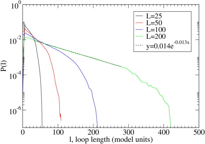
For each pair of connected footpoints, we measured the length of the loop linking them, irrespective of the strength of the link. This was done according to the definition of loop length in section 2.2. The distribution of loop lengths measured in numerical simulations is shown in Figure 9. The loop lengths appear to be exponentially distributed from approximately $0.05\pi L<l<0.45\pi L$, i.e.

$$P(l)\sim e^{-l/\xi(m,L)}$$

where $\xi(m,L)$ is the characteristic length of a loop. In Table 4.3, $\xi$ is determined by fitting to the data for each system size between $0.05\pi L$ and $0.45\pi L$ using least squares analysis. The fit to an exponential in this range is extremely good (e.g. $r>0.997$ for $L=200$). Occasionally loops extend up to the maximum possible size $\pi L/\sqrt{2}$. Increasing the system size, $L$, not only increases the maximum observed loop length, but also changes $\xi$. As shown in table , there is a weak dependence of $\xi$ on the stirring rate $m$ for a fixed system size $L$.

As flux tubes in our model are described as semi-circular loops normal to the photosphere, the footpoint separation and maximum loop height are also exponential distributions, trivially related to $P(l)$.

Close et al calculated flux tube statistics from magnetograms based on a potential field approximation. Figures 10 and 11 compare their results for footpoint separation and maximum height of flux tubes with Models I and II. Note that both of these figures show the cumulative distributions.

Reanalysis of the footpoint separation data from Close et al reveals that the probability distribution of footpoint separations follows an exponential with a characteristic length of $20\pm 3$Mm.

Figure 10: The cumulative percentage of pairs of connected concentrations separated by a distance larger than $d$. The flux tube data corresponds to Figure 6c in Close et al. (2003). The model data has been scaled such that one unit of length is equal to 0.5Mm. Good agreement is found for separations up to the typical supergranule diameter, 15Mm. The parameters used were $m=0.1,L=100$ for model I and $m=1,L=100$ for model II.

Figure 11: The cumulative percentage of maximum loop heights larger than a certain amount. The flux tube data corresponds to Figure 6b from Close et al. (2003). The model data has been scaled such that one unit of length is equal to 0.5Mm, as in Figure 10. Agreement between the two data sets is poor, and the range of heights obtained by Close et al. (2003) under the potential field approximation is larger than is possible with our model with the given parameters. The parameters used were $m=0.1,L=100$ for model I and $m=1,L=100$ for model II.

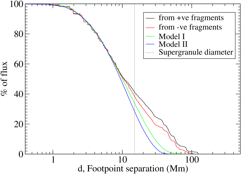
4.3.1 Calibration

Figure 10 demonstrates how the unit length of the model can be calibrated to actual lengths on the photosphere. Comparing the cumulative distribution of the model to Close et al, and setting one unit of length in the model equal to 0.5Mm for $L=100$, the cumulative distribution of footpoint separations agree up to the supergranule cell size, (15Mm). Beyond that length scale, the distributions do not agree. This difference may be due to the finite size effects in the model and/or the potential field approximation used to determine the flux tubes.

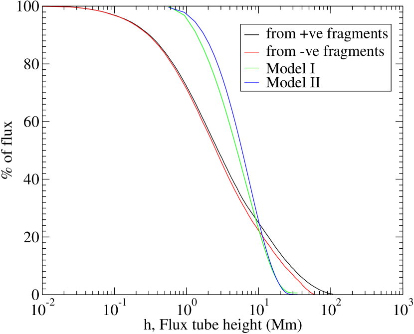
4.3.2 Flux tube heights

Figure 11 shows the cumulative distribution of maximum loop heights for model I and II compared to the flux tube heights measured by Close et al. Using the same calibration factor as determined for lengths in Figure 9, the results from the numerical simulations do not agree with the measurements over the entire range. Although the distributions have roughly the same shape, the heights calculated by Close et al extend over a much wider range than is seen or is indeed possible in the model discussed here. This disagreement is not particularly surprising. The semi-circular loops in our model are always perpendicular to the photosphere, so that the maximum height attained is simply the radius of the loop. Under the potential field approximation, the maximum height a loop can attain is not simply related to the footpoint separation. For example the loop can trace out a very flat curve, lying close to the photosphere. However, TRACE images tend to qualitatively support the picture of flux tubes emerging perpendicular to the photosphere.

4.4 Emergence rate and turnover time

m	$\xi$ (model units)	$\langle N\rangle$	$\langle N_{loops}\rangle$
0.001	22	549	1100
0.01	31	358	720
0.1	40	190	391
1	43	83	139

Table 1: Average number of footpoints $\langle N\rangle$, average number of loops $\langle N_{loops}\rangle$ and characteristic loop length $\xi$ in model I for different values of $m$, with system size $L=100$. Note that $\xi$ depends very weakly on $m$.

In order to determine the predicted flux turnover time for the Sun we need to calibrate not only the units of distance but also of time in the model. The length calibration was determined earlier to be one unit of length equal to 0.5Mm for Model I with $m=0.1,L=100$. Strictly this calibration varies for different values of $m$. However, as can be seen in table 1 the characteristic loop length $\xi$ only changes by a factor of about 2, while $m$ is varied over 3 orders of magnitude. Therefore the effect of changing $m$ on the length scale is very small and is ignored in the calculation that follows.

Hagenaar et al. (1999) observe that magnetic concentrations diffuse on the photosphere. Footpoints in our model also diffuse. They execute a random walk with the distance moved in each discrete time step drawn from a uniform probability distribution between 0 and 1, or 0 to 0.5Mm after calibration for $L=100$. The mean square displacement of the footpoints in one step is therefore 0.083Mm². During a parallel update step each footpoint moves once on average, therefore a parallel update step is equal to N single footpoint updates, where N is the total number of footpoints in the system. We denote the length of time taken for a parallel update step as $\Delta t$. From Figure 2 in Hagenaar et al. (1999), the mean square displacement of 0.083Mm² is observed to take approximately 300 seconds. We therefore set $\Delta t=300$secs$=0.083$hrs.

The parameter $m$ measures the fraction of footpoints moved between loop injections, therefore in one parallel update step $1/m$ loops are added. The number of loops injected per hour is given by

$$loops/hour=\frac{1}{m\Delta t},$$ (8)

where $\Delta t$ is measured in hours.

We determine the turnover time, $t_{turnover}$, from the average number of loops in the system, $\langle N_{loops}\rangle$, and the number of loops injected per hour by the following formula:

$$t_{turnover}=\frac{\langle N_{loops}\rangle}{loops/hour}=m\Delta t\langle N_{loops}\rangle.$$ (9)

The turnover times for model I and II are shown in tables 2, and 3 respectively. Note that the flux calibration used in Figure 3 is not relevant to this calculation.

As seen in tables 2 and 3 and expressed in equation 9, the turnover time depends on the stirring rate $m$. However in model I, which includes the cancelation of concentrations on the photosphere, the turnover time has a much stronger dependence on the stirring rate than it does in model II, which does not allow the cancelation of concentrations. At this point in time we have no a priori reason to select model I or model II or a particular stirring rate, so we cannot make a completely definitive statement as to the expected turnover time.

However it is reasonable to expect that the dimensionless parameter $m$, that characterizes how the flux is driven in the system, should be neither extremely large or extremely small. If $m$ is very large then essentially all the flux is removed from the system and the density of footpoints is vanishingly small. While if $m$ is very small then the footpoints barely move and cannot be observed to diffuse during their lifetime. The fact that we see flux emerging as well as the diffusion of concentrations indicates that $m$ should be approximately within the range of values shown in tables 2 and 3.

4.4.1 Emergence rate

Tables 2 and 3 also show the flux emergence rate and total amount of flux for the entire solar surface estimated from the numerical simulation results as explained below. Unlike the turnover time, these estimates require the calibration of flux in the model to measurable flux on the photosphere. We use the same calibration as in Figure 3. One unit of flux is equal to $1.55\times 10^{17}$Mx, which is the threshold resolution of Close et al. The results from the simulations were scaled up to the entire solar area by assuming the system of size $L$ represents a typical section of the photosphere. Thus the flux values are multiplied by the ratio of the total photospheric surface area to the model surface area (50Mm$\times$50Mm for $L=100$).

m	emergence	total flux	$t_{turnover}$
	rate (Mx/hr)	(Mx)	(hr)
0.001	$5\times 10^{24}$	$5\times 10^{23}$	0.1
0.01	$5\times 10^{23}$	$3\times 10^{23}$	0.6
0.1	$5\times 10^{22}$	$2\times 10^{23}$	3
1	$5\times 10^{21}$	$6\times 10^{22}$	12

Table 2: Average flux emergence rate, total amount of flux, and flux turnover time in model I with $L=100$, scaled to represent the total surface area of the Sun.

m	emergence	total flux	$t_{turnover}$
	rate (Mx/hr)	(Mx)	(hr)
0.1	$5\times 10^{22}$	$6\times 10^{23}$	12
1	$5\times 10^{21}$	$1\times 10^{23}$	25
10	$5\times 10^{20}$	$3\times 10^{22}$	63

Table 3: Average flux emergence rate, total amount of flux, and flux turnover time in model II with L=100, scaled to represent the total surface area of the Sun.

It is immediately clear that the total flux does not vary linearly with $m$, although by equation 8 the rate of flux emergence does. This means that the model can exhibit a range of flux turnover times on changing $m$. This agrees with the physical picture where higher injection rates (when $m$ is small) result in systems with a higher loop and footpoint density, making interactions more frequent. In particular, concentration cancelation in model I will occur more often (relative to parallel update steps) and hence loop lifetimes will be reduced and flux turnover times decreased. This explains why model I has a stronger dependence of turnover time on the stirring rate $m$.

4.4.2 Comparison with observations

Studies measuring the rate of flux emergence have determined rates which vary widely, from e.g. $\sim 4\times 10^{20}$Mx/hr (Harvey 1993), to $\sim 2\times 10^{22}$Mx/hr (Hagenaar 2001). Later studies have tended to indicate a higher rate of flux emergence, as ever smaller flux concentrations are resolved and included in the analysis. The estimates of total solar flux have hardly changed over the same time period, usually quoted as being no less than $\sim 3\times 10^{23}$Mx (e.g. Schrijver et al. (1997)). The figures for flux turnover rates have therefore correspondingly decreased over time. The recent measurements by Hagenaar et al. (2003) suggest a turnover time of 8-19 hours, much shorter than the 40-70 hours from a few years earlier (Schrijver et al. 1997).

Both model I and II give total flux values comparable with the estimates of total solar flux, and both also give turnover times which are compatible with current estimates. However it is necessary that one uses the same $m$ value for both the total flux and the turnover time. This suggests that, based on current estimates of the emergence rate and total flux, model II is a better description of the coronal magnetic network than model I. Model II with $m\simeq 0.3$ agrees quantitatively with the current estimates for both the total flux and the flux turnover time.

Thus the cancelation of concentrations may be a less important process in the dynamics.

5 Conclusions

The main results of this work are as follows:

• Observational data of magnetic concentration strengths on the photosphere were reanalyzed. We found that the distribution of concentration strengths exhibits power law behavior, with a critical exponent $\gamma\sim 1.7$, in the range $2-500\times 10^{17}$Mx. This distribution is compatible with that of active region areas, which have much larger flux values.

• We conjecture that a single power law describes the distribution of magnetic concentrations of all sizes, from the smallest detectable fragments to large active regions. The power law distribution at sufficiently large scales is cutoff by the finite size of the Sun, as is typical in critical finite size systems.

• We propose that the coronal magnetic field embodies a scale free network. Concentrations on the photosphere are nodes in the network. They are linked by flux tubes. The distribution of magnetic concentration strengths therefore corresponds to the degree distribution of a network, and it is scale free with an exponent $\gamma$.

• A self organized critical model involving avalanches of reconnecting flux tubes generates a scale free magnetic network. The distribution of concentration strengths measured in numerical simulations of the model agrees quantitatively with the reanalyzed observational data presented here. A single calibration is required that sets the unit of flux in the model equal to the threshold magnetic flux that can be presently detected on the photosphere. Otherwise there is no fitting parameter.

• This model exhibits a power law distribution of flare events (Hughes et al. 2003). Thus the scale free behavior of flares and of magnetic concentrations are unified in terms of a single dynamical process, which self generates the complex magnetic field structure and dynamics.

• Two new quantities are introduced to characterize scale free networks. Both of these quantities can be measured for the corona. The strength of a connection between two nodes can be distributed as a power law, with an exponent $\alpha\geq\gamma$. In the model this distribution is found to be scale free. We propose that the amount of flux connecting two concentrations on the photosphere has power law behavior with an exponent $\alpha$. Also the number of unique concentrations linked to any concentration by flux tubes also has a scale free distribution, with a different exponent.

• The distribution of flux tube lengths measured in numerical simulations of the model and observed in the corona is exponential up to the supergranule cell size. This allows a calibration of the length unit of the model to a physical length on the photosphere. Furthermore the observed diffusive behavior of concentrations on the photosphere allows us to then calibrate the time unit of the model.

• Based on these calibrations we determine the flux turnover time and the total coronal flux that the model predicts. Our results are compatible with current estimated values for the Sun.

We thank R. Close and H.J. Hagenaar for generously sending us their previously published observational data. We would like to thank R. Dendy and S.C. Cowley for their comments, and P. Hanlon for his assistance with data processing. D. Hughes acknowledges funding from EPSRC.

References

- Albert & Barabási (2002) Albert, R. & Barabási, A. L. 2002, Rev. Mod. Phys., 74, 47
- Aschwanden et al. (2000) Aschwanden, M., Tarbell, T. D., Nightingale, R. W., Schrijver, C. J., Title, A., Kankelborg, C., Martens, P., & Warren, H. 2000, Astrophys. J., 535, 1047
- Bak (1996) Bak, P. 1996, How Nature Works: The Science Of Self-Organized Criticality (Copernicus, New York)
- Bak et al. (1987) Bak, P., Tang, C., & Weisenfeld, K. 1987, Phys. Rev. Lett., 59, 381
- Barabasi & Albert (1999) Barabasi, A.-L. & Albert, R. 1999, Science, 286, 509
- Bornholdt & Schuster (2002) Bornholdt, S. & Schuster, H. G., eds. 2002, Handbook on graphs and networks (Wiley-VCH)
- Close et al. (2003) Close, R., Parnell, C., MacKay, D., & Priest, E. 2003, Sol. Phys., 212, 251
- Faloustos et al. (1999) Faloustos, M., Faloustos, P., & Faloustos, C. 1999, Comput. Commun. Rev., 29, 251
- Frette et al. (1996) Frette, V., Christensen, K., Malthe-Sørenssen, A., Feder, J., Jøssang, T., & Meakin, P. 1996, Nature, 379, 49
- Hagenaar (2001) Hagenaar, H. J. 2001, ApJ, 555, 448
- Hagenaar et al. (2003) Hagenaar, H. J., Schrijver, C. J., & Title, A. M. 2003, ApJ, 584, 1107
- Hagenaar et al. (1999) Hagenaar, H. J., Schrijver, C. J., Title, A. M., & Shine, R. A. 1999, ApJ, 511, 932
- Harvey (1993) Harvey, K. L. 1993, Ph.D. Thesis
- Harvey & Zwaan (1993) Harvey, K. L. & Zwaan, C. 1993, Sol. Phys., 148, 85
- Hughes & Paczuski (2002) Hughes, D. & Paczuski, M. 2002, Phys. Rev. Lett., 88, 054302
- Hughes et al. (2003) Hughes, D., Paczuski, M., Dendy, R. O., Helander, P., & McClements, K. G. 2003, Phys. Rev. Lett., 90, 131101
- Livi et al. (1985) Livi, S. H. B., Wang, J., & Martin, S. F. 1985, Australian Journal of Physics, 38, 855
- Lu & Hamilton (1991) Lu, E. & Hamilton, R. 1991, ApJ, 380, L89
- Maslov & Sneppen (2002) Maslov, S. & Sneppen, K. 2002, Science, 296, 910
- Parker (1994) Parker, E. 1994, Spontaneous Current Sheets in Magnetic Fields (New York: Oxford University Press)
- Priest & Forbes (2000) Priest, E. & Forbes, T. 2000, Magnetic Reconnection (Cambridge: Cambridge University Press)
- Redner (1998) Redner, S. 1998, Eur. Phys. J. B., 4, 131
- Schrijver et al. (1997) Schrijver, C. J., Title, A. M., van Ballegooijen, A. A., Hagenaar, H. J., & Shine, R. A. 1997, ApJ, 487, 424
- Wagner (2001) Wagner, A. 2001, Mol. Biol. Evol., 18, 1283