Dynamical Effects from Asteroid Belts for Planetary Systems

Abstract

The orbital evolution and stability of planetary systems with interaction from the belts is studied using the standard phase-plane analysis. In addition to the fixed point which corresponds to the Keplerian orbit, there are other fixed points around the inner and outer edges of the belt. Our results show that for the planets, the probability to move stably around the inner edge is larger than the one to move around the outer edge. It is also interesting that there is a limit cycle of semi-attractor for a particular case. Applying our results to the Solar System, we find that our results could provide a natural mechanism to do the orbit rearrangement for the larger Kuiper Belt Objects and thus successfully explain the absence of these objects beyond 50 AU.

Keywords: Phase-plane analysis; bifurcation; planetary systems; stellar dynamics.

1 Introduction

Newton’s Law of gravity and motion has been used as the most fundamental law for the Physical Sciences since its success in explaining the motion of celestial bodies in the Solar System. Thus, the Newton’s Law was in fact first proved in the astronomical context. It was then applied to other fields successfully.

For example, Clausen et al. [1998] studied periodic modes of motion of a few body system of magnetic holes, both experimentally and numerically. Kaulakys et al. [1999] showed that a system of many bodies moving with friction can experience a transition to chaotic behavior. Xia [1993] did some work on Arnold diffusion in the elliptic restricted three-body problems.

Many new discoveries of extrasolar planets have been made recently (Marcy et al. [1997]) and these events really provide exciting and important opportunities to understand the formation and evolution of planetary systems, including the Solar System. According to the Extrasolar Planets Catalog (http://cfa-www.harvard.edu/planets/catalog.html) maintained by Jean Schneider, 117 planets have been detected till date (July 2003). These planets have masses ranging from 0.16 to 17 Jupiter mass ($M_{J}$) and semimajor axes ranging from 0.04 AU to 4.5 AU and a wide range of eccentricities. Therefore, the dynamical properties of some of these planets are very different from the planets in the Solar System.

Nevertheless, there do exist similarities between the extrasolar and the Solar System planets. For example, there is a new discovery of a Jupiter-like orbit, i.e. a Jupiter-mass planet on a circular long-period orbit (Marcy et al. [2002]). Moreover, some planetary systems are claimed to have discs of dust and they are regarded to be young analogues of the Kuiper Belt in our Solar System (Jayawardhana et al. [2000]).

If these discs are massive enough, they should play important roles in the origin of planets’ orbital elements. In fact, Terquem & Papaloizou [2002] provide an important mechanism to explain the observed planetary systems: massive planets form at the inner part of the system and move on a circular orbit due to tidal interaction with the disc, whereas lower mass planets form at the outer part and interact with the inner ones. Thus, the eccentricities of the massive inner planets increase, which is in accord with the observations. Moreover, the simulations in Jiang & Ip [2001] show that the orbital configuration of the planetary system of upsilon Andromedae might initially be caused by the disc interaction. Although the discs might be depleted and gradually become less massive, there could be belts surviving until now as the Asteroid and Kuiper Belts in the solar system and these belts would be important for whole dynamical histories of planets.

On the other hand, Thommes, Duncan & Levison [1999] claimed that Neptune was closer to Jupiter and got scattered outward. Yeh & Jiang [2001] studied the orbital migration of scattered planets and completely classified the parameter space and the solutions. They concluded that the eccentricity always increases if the planet which moves on a circular orbit initially, is scattered to migrate outward. Thus, the orbital circularization must be important for the scattered planets if they are now moving on nearly circular orbits.

Since belts of planetesimals often exist within a planetary system and provide the possible mechanism of orbital circularization, it is important to understand the solutions of dynamical systems with planet-belt interaction. Therefore, Jiang & Yeh [2003] did some analysis of the solutions for dynamical systems of planet-belt interaction for a belt with simple density profile $c/r$, where $c$ is a constant. However, because the gravitational force from the belt involves complicated elliptic integrals and is difficult for the construction of theorems, they used simplified analytic formulas to estimate this force. Their main conclusion is that the inner edge of the belt is more stable than the outer edge of the belt for the planets. Their result is actually consistent with the observational picture of the Asteroid Belt.

In this paper, we complete the work initiated in our earlier paper Jiang & Yeh [2003], by numerically evaluating elliptic integrals to obtain the gravitational force of the belt without introducing any simplifications. Thus, this study is intended to improve the understanding about orbital evolution of a given planet-belt system and hopefully explain why there are less Kuiper Belt Objects larger than 160 km in diameter beyond 50 AU in the outer Solar System. In Section 2, we mention our basic governing equations and in Section 3, we study the locations of the fixed points. The phase-plane analysis is discussed in Section 4 and Section 5 concludes the paper.

2 The Model

The belt is an annulus with inner radius $r_{1}$ and outer radius $r_{2}$, where $r_{1}$ and $r_{2}$ are assumed to be constants. According to Lizano & Shu [1989], the belt’s surface density scales with distance as $r^{-2}$. We thus assume the density profile of the belt to be $\rho(r)={c}/{r^{2}}$, where $c$ is a constant, completely determined by the total mass of the belt. One might notice that there are discontinuities at $r=r_{1}$ and $r=r_{2}$. This is probably acceptable because the edges of the belt are rather sharp as one can see from a plot of the Asteroid Belt in Murray & Dermott [1999].

The units of length and time are chosen so as to easily compare with our Solar System. There are two belts for our Solar System: the Asteroid Belt in the inner part of the Solar System and the Kuiper Belt in the outer part. We set $r_{1}=3$ and $r_{2}=6$ because (1) when the length unit is 1 AU (and the time unit is $1/(2\pi)$ years), the interval $[r_{1},r_{2}]$ covers the region of the Asteroid Belt approximately, (2) when the length unit is 10 AU (and the time unit is $10^{3/2}/(2\pi)$ years), the interval $[r_{1},r_{2}]$ covers the region of the Kuiper Belt.

We assume the distance between the central star and the planet to be $r$, where $r$ is a function of time. The total force $f$ acting on the planet, includes the contributions from the central star and the belt. The gravitational force from the central star is

$$f_{s}=-\frac{m}{r^{2}},$$ (1)

where we have set the mass of the central star to be 1 and also the gravitational constant $G=1$.

On the other hand, the gravitational force from the belt for the planet is complicated and involves elliptic integrals. We use the equations in Appendix A to get the force $f_{b}$ numerically.

Because there might be some scattering between the planetesimals in the belt and the planet, the planet should experience the frictional force when it goes into the belt region. This frictional force should be proportional to the surface density of the belt at the location of the planet, and the velocity of the planet. However, if the planet is doing circular motion, the probability of close encounter between the planet and the planetesimals in the belt is very small and can be neglected here. Thus, we can assume that the frictional force is proportional to the radial velocity of the planet $dr/dt$ only, and ignore the $d\theta/dt$ dependence.

Therefore, the frictional force $\tilde{f}_{\alpha}$ is proportional to the surface density of the belt and radial velocity $dr/dt$. Hence, we write down the formula for frictional force as

$$\tilde{f}_{\alpha}=-\alpha\rho(r)\frac{dr}{dt},$$ (2)

where $\alpha$ is a frictional parameter and $\rho$ is the density profile of belt.

Because the $d\theta/dt$ component of the planetary velocity is ignored in the frictional force, the angular momentum $l$ is conserved here, so we have

$$mr^{2}{d\theta}=l{dt}.$$ (3)

This implies that Kepler’s second law is still valid here and, because of this, we can use $\theta$ as our independent variable. We use $\theta$ to label time $t$ from now on and one can easily get $t$ from the above equation.

Since $u=1/r$ and using Equation (3), we have

$$\frac{dr}{dt}=\frac{dr}{d\theta}\frac{d\theta}{dt}=\frac{l}{mr^{2}}\frac{dr}{d\theta}=-\frac{l}{m}\frac{du}{d\theta}.$$ (4)

Equation (2) can be rewritten as

$$\tilde{f}_{\alpha}=-\alpha\rho(r)\left[-\frac{l}{m}\frac{du}{d\theta}\right]=\frac{\alpha l\rho}{m}\frac{du}{d\theta}.$$ (5)

Since the planet feels the frictional force only when it enters the belt region, we define

$$f_{\alpha}=\beta\tilde{f}_{\alpha},$$ (6)

where

$$\beta=\left\{\begin{array}[]{ll}1&{\rm if}\quad r_{1}<r<r_{2},\\ 0&{\rm if}\quad r>r_{2}\quad{\rm or}\quad r<r_{1}.\end{array}\right.$$

In general, the equation of motion for the planet is (Goldstein [1980])

$$\frac{d^{2}u}{d\theta^{2}}=-u-\frac{mf\left(\frac{1}{u}\right)}{l^{2}u^{2}},$$ (7)

where $u=1/r$ and $m$, $l$ are the mass and the angular momentum of the planet and $f$ is the total force acting on the planet. This equation is only valid when there is no non-radial force. We use the polar coordinates $(r,\theta)$ to describe the location of the planet.

Because $f=f_{s}+f_{b}+f_{\alpha}$, we transform Equation (7) into

$$\frac{d^{2}u}{d\theta^{2}}=-u+\frac{m^{2}}{l^{2}}-\frac{m^{2}f_{b}}{l^{2}u^{2}}-\frac{\beta\alpha\rho}{lu^{2}}\frac{du}{d\theta}.$$ (8)

Therefore, the equation of motion for this system can be written as

$$\frac{du}{d\theta}=v\equiv g_{1}(u,v),$$

$$\frac{dv}{d\theta}=-u-\beta k_{1}\frac{\rho}{u^{2}}v+k_{2}-k_{2}\frac{f_{b}}{u^{2}}\equiv g_{2}(u,v),$$ (9)

where $k_{1}\equiv{\alpha}/{l}$, $k_{2}\equiv m^{2}/l^{2}$.

3 Fixed Points

The fixed points $(u,v)$ of Equation (9) satisfy the following equations :

$$v=0,$$

$$-u-\beta k_{1}\frac{\rho}{u^{2}}v+k_{2}-k_{2}\frac{f_{b}}{u^{2}}=0.$$ (10)

From Equation (10), the fixed points $(u,0)$ satisfy

$$u^{3}-k_{2}u^{2}+k_{2}f_{b}=0.$$ (11)

The fixed points can be numerically determined for any given $k_{2}$ and $f_{b}$ and it is obvious that the location of fixed points does not depend on the friction. Since at fixed points $v=du/d\theta=0$, the fixed points correspond to circular orbits. Particularly, when $f_{b}=0$, by Equation (11), the fixed point satisfies $u=k_{2}$ and this actually corresponds to the Keplerian orbit. (One can check easily by writing $k_{2}$ as a function of usual angular velocity.)

The density profile of the belt is $\rho(r)={c}/{r^{2}}$, where $c$ is determined by the total mass of the belt (Lizano & Shu [1989]). Hence, the total mass of the belt is

$$M_{b}=\int^{2\pi}_{0}\int^{r_{2}}_{r_{1}}\rho(r^{\prime})r^{\prime}dr^{\prime}d\phi=2\pi c(\ln r_{2}-\ln r_{1}).$$ (12)

From Appendix A, we can then calculate $f_{b}$ for any given total mass of the belt $M_{b}$ as the constant $c$ can be uniquely determined from $M_{b}$. Moreover, since $m$ is always $0.001$ (about $M_{J}$) in this paper, $k_{2}$ is directly related to the angular momentum of the planet. Therefore, we use $M_{b}$ and $k_{2}$ as the two main parameters to determine the number and locations of fixed points in this system.

Figure 1 is the bifurcation diagram of fixed points and these curves show the locations of fixed points $u$ as a function of $k_{2}$ for a given $M_{b}$. From this plot, we know that when the total mass of the belt is very small, $M_{b}=0.01$, the curve on the $k_{2}-u$ plane is almost a straight line with slope 1. That is, there is one and only one fixed point $u\sim k_{2}$. This can be easily verified by Equation (11) with small $f_{b}$, and it corresponds to the Keplerian orbits. When the mass of the belt is not negligible, the curves form two needle-like structures pointing along both, the inner edge of the belt, where $u=1/r_{1}=1/3$, and the outer edge of the belt, where $u=1/r_{2}=1/6$, and there would be more than one fixed point for particular values of $k_{2}$. In addition to the one corresponding to the Keplerian orbit, other fixed points are located around inner and outer edges of the belt. Thus, the belt could bring the planets to non-Keplerian circular orbits by the gravitational and frictional forces.

When $M_{b}=0.1$, the needle-like structures imply the existence of two fixed points for $0.5<k_{2}<0.7$. When $M_{b}=0.5$, the two needle-like structures become even bigger and there are three fixed points for $0.5<k_{2}<1$ , two fixed points around $k_{2}=0.06$ and one fixed point for most other values of $k_{2}$. When $M_{b}=1$, the structure grows even larger and becomes completely different from a straight line. There are three fixed points for larger $k_{2}$ ($k_{2}>0.6$) and one fixed point only for both intermediate $k_{2}$ ($0.1<k_{2}<0.5$) and tiny $k_{2}$ ($k_{2}<0.02$). Since the needle-like structure around the outer edge is tiny, the probability that the planet moves stably around the outer edge is much smaller than near the inner edge.

4 Phase-Plane Analysis

Following the linearization analysis, the eigenvalues $\lambda$ corresponding to the fixed points $(u_{\ast},0)$ satisfy the following equation:

$$\left(\frac{\partial g_{1}}{\partial u}\biggm{|}_{(u_{\ast},0)}-\lambda\right)\left(\frac{\partial g_{2}}{\partial v}\biggm{|}_{(u_{\ast},0)}-\lambda\right)-\left(\frac{\partial g_{1}}{\partial v}\biggm{|}_{(u_{\ast},0)}\right)\left(\frac{\partial g_{2}}{\partial u}\biggm{|}_{(u_{\ast},0)}\right)=0,$$ (13)

where $g_{1}(u,v)=v$ and $g_{2}(u,v)=-u-\beta{(k_{1}\rho v)}/{u^{2}}+k_{2}-{(k_{2}f_{b})}/{u^{2}}$. Hence, the above equation becomes

$$\lambda^{2}+\frac{\beta k_{1}\rho}{u_{\ast}^{2}}\lambda+\left(1-\frac{2\beta k_{1}\rho v}{u^{3}}\biggm{|}_{(u_{\ast},0)}+k_{2}\frac{\partial A}{\partial u}\biggm{|}_{(u_{\ast},0)}\right)=0,$$

$${\rm where}\,\,A=\frac{f_{b}}{u^{2}}.$$ (14)

When the planet is out of the belt region, that is $\beta=0$, we have

$$\lambda=\pm\sqrt{-1-k_{2}\frac{\partial A}{\partial u}\biggm{|}_{(u_{\ast},0)}},$$

and there are two possible cases:

Case I: If $-1-k_{2}\frac{\partial A}{\partial u}\biggm{|}_{(u_{\ast},0)}>0$, this fixed point is a saddle point.

Case II: If $-1-k_{2}\frac{\partial A}{\partial u}\biggm{|}_{(u_{\ast},0)}<0$, this fixed point is a center point.

When the planet stays in the belt, that is $\beta=1$, we have

$$\lambda=\frac{k_{1}\rho}{2u_{\ast}^{2}}\left\{-1\pm\sqrt{1-4\left(1+k_{2}\frac{\partial A}{\partial u}\biggm{|}_{(u_{\ast},0)}\right)\left(\frac{u_{\ast}^{2}}{k_{1}\rho}\right)^{2}}\right\}.$$

We define $\Delta={1-4\left(1+k_{2}\frac{\partial A}{\partial u}\biggm{|}_{(u_{\ast},0)}\right)\left(\frac{u_{\ast}^{2}}{k_{1}\rho}\right)^{2}}$, then we have three possible cases:

Case 1: When $\Delta<0$, two eigenvalues $\lambda_{1,2}=-a\pm b{\rm i}$ for $a,b>0$, so the fixed point is a stable spiral point.

Case 2: When $0<\Delta<1$, both eigenvalues are negative, so the fixed point is a stable node.

Case 3: When $\Delta>1$, one eigenvalue is negative and the other is positive, so the fixed point is a saddle point.

We understand that when the real parts of the eigenvalues of a fixed point equal to zero in the first-order linearization analysis, the properties of this fixed point should be determined by the higher order analysis in general. However, to simplify our language, we still use the term “center point” for any fixed point having an eigenvalue with zero real part. This is a good choice because our numerical results indicate that these points are in fact the center points.

We now derive the mathematical formula for $\Delta$. At first, from Equation (14), we calculate (please see details in Appendix B)

$$\frac{\partial A}{\partial u}\biggm{|}_{(u_{\ast},0)} = \frac{1}{u_{\ast}^{2}}\frac{\partial f_{b}}{\partial u}\biggm{|}_{(u_{\ast},0)}-\frac{2f_{b}}{u_{\ast}^{3}}=-\frac{1}{u_{\ast}^{4}}\frac{\partial f_{b}}{\partial r}\biggm{|}_{(u_{\ast},0)}-\frac{2f_{b}}{(u_{\ast})^{3}},$$ (15)

$$= -\frac{2}{u_{\ast}}\int_{r^{\prime}}r^{\prime}\rho(r^{\prime})\left\{\frac{1+r^{\prime 2}u_{\ast}^{2}}{(1-r^{\prime}u_{\ast})^{2}(1+r^{\prime}u_{\ast})}E-\frac{1}{1+r^{\prime}u_{\ast}}F\right\}dr^{\prime},$$

where $E$ is an elliptic integral of the second kind and $F$ is an elliptic integral of the first kind. Hence, we have

$$\Delta = 1-4\left(\frac{u_{\ast}^{2}}{k_{1}\rho}\right)^{2}\left(1+k_{2}\frac{\partial A}{\partial u}\biggm{|}_{(u^{\ast},0)}\right)$$ (16)

$$= 1-4\left(\frac{u_{\ast}^{2}}{k_{1}\rho}\right)^{2}\left\{1-\frac{2k_{2}}{u_{\ast}}\int_{r^{\prime}}r^{\prime}\rho(r^{\prime})\left[\frac{1+r^{\prime 2}u_{\ast}^{2}}{(1-r^{\prime}u_{\ast})^{2}(1+r^{\prime}u_{\ast})}E-\frac{1}{1+r^{\prime}u_{\ast}}F\right]dr^{\prime}\right\}$$

$$= 1-4\left(\frac{u_{\ast}^{2}}{k_{1}\rho}\right)^{2}+\frac{8u_{\ast}^{3}k_{2}}{k_{1}^{2}\rho^{2}}\int_{r^{\prime}}r^{\prime}\rho(r^{\prime})\left[\frac{1+r^{\prime 2}u_{\ast}^{2}}{(1-r^{\prime}u_{\ast})^{2}(1+r^{\prime}u_{\ast})}E-\frac{1}{1+r^{\prime}u_{\ast}}F\right]dr^{\prime}.$$

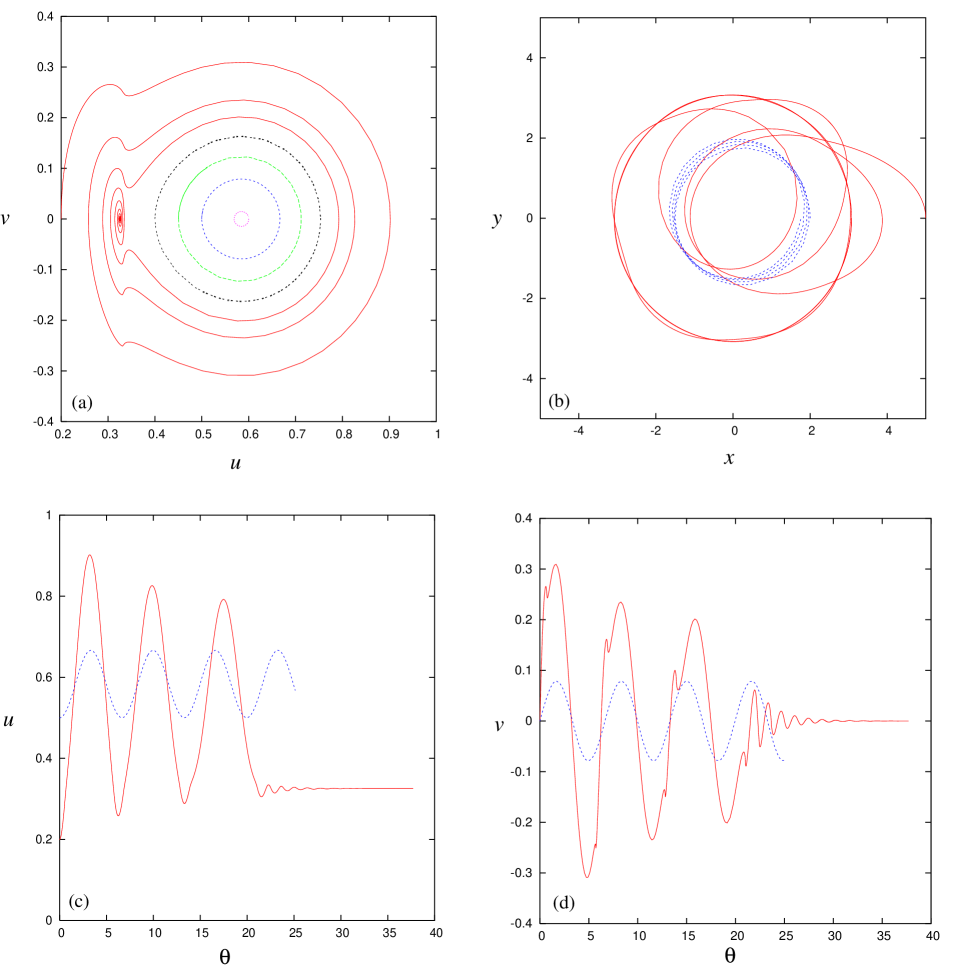
Figure 2: The result for $M_{b}=0.5$ and $k_{2}=0.6$ with $\alpha=0.001$, $r_{1}=3$, $r_{2}=6$. (a) Solution curves on the $u-v$ phase-plane. (b) Orbits on the $x-y$ plane. (c) The plots of $u$ as a function of $\theta$. (d) The plots of $v$ as a function of $\theta$. The red solid (blue dotted) curves in all panels correspond to the same solution.

If we calculate the value of $\Delta$ numerically, we can then understand the properties of this fixed point. For example, in Figure 2-6, we choose four sets of ($M_{b}$, $k_{2}$) values and make the phase-plane plots, orbits etc. to demonstrate the orbital evolution, and the stability of the system to provide a general picture for the readers. In the results below, the frictional parameter $\alpha$ were chosen to be small numbers but large enough to make the solution curve not too tight to be studied. The value of the frictional parameter $\alpha$ is related to the viscosity of the belt and is too complicated to be well-determined observationally. The values of $\alpha$ in the models would affect the time scales of orbital evolution but would not change the general understanding of the dynamical properties of the system. For the parameters we choose, some results show that the orbits become nearly circular in an order of $10^{3}$ years if the unit of length is 10 AU. This is rather short and perhaps only possible during the period in which the planetary system is just formed. Nevertheless, one can easily choose smaller values of $\alpha$ to get results of orbital evolution with longer time scales when the results are used to describe more recent systems.

Figure 2 is the case when we set $M_{b}=0.5$ and $k_{2}=0.6$. We assume the frictional parameter $\alpha=0.001$ for this case. We know from Figure 1, that there must be three fixed points and Figure 2(a) shows that the one around $u=0.6$ is a center point and the other two near the inner edge of the belt are spiral and saddle points, respectively. The blue dotted curve around the center point in Figure 2(a) is then plotted on the $x-y$ plane as the blue dotted orbit in Figure 2(b). It is a precessing elliptical orbit with small eccentricity. The red solid curve approaching the spiral point in Figure 2(a) is then plotted on the $x-y$ plane as the red solid orbit in Figure 2(b). This orbit keeps changing the semimajor axis and eccentricity and finally becomes a circular orbit with radius $r=r_{1}$, i.e., close to the inner edge of the belt. Figures 2(c)-(d) show $u$ and $v$ as functions of $\theta$ for both above orbits. Because $u$ becomes a constant and $v$ approaches to zero when $\theta>30$ for the red solid curves in Figures 2(c)-(d), these two figures reconfirm that the red solid curve in Figure 2(b) finally becomes a circular orbit. While, since both $u$ and $v$ keep oscillating for the blue dotted curves in Figures 2(c)-(d), the blue dotted curve in Figure 2(b) is then a precessing elliptical orbit.

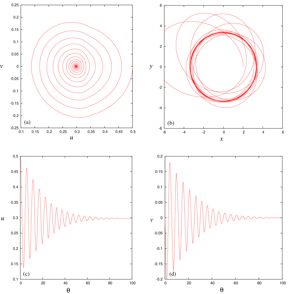
Figure 3: The result for $M_{b}=0.1$ and $k_{2}=0.3$ with $\alpha=0.01$, $r_{1}=3$, $r_{2}=6$. (a) A solution curve on the $u-v$ phase-plane. (b) An orbit on the $x-y$ plane. (c) The plot of $u$ as a function of $\theta$. (d) The plot of $v$ as a function of $\theta$. The curves in all panels correspond to the same solution.

Figure 3 is the case when we set $M_{b}=0.1$ and $k_{2}=0.3$. We assume the frictional parameter $\alpha=0.01$ for this case. From Figure 1, we know that there is only one fixed point and it is close to the inner edge of the belt, where $u=1/r_{1}=1/3$. Figure 3(a) shows that this fixed point is a spiral point. The solution curve on the $u-v$ phase-plane is then plotted as an orbit on the $x-y$ plane in Figure 3(b). We can see that the planet moves across the belt initially and gradually settles down on a circular orbit close to the inner edge of the belt. Figures 3(c)-(d) show $u$ and $v$ as functions of $\theta$ for this orbit.

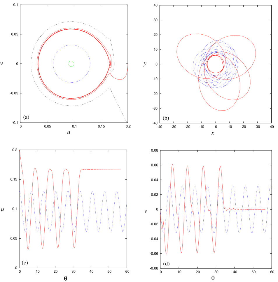
Figure 4: The result for $M_{b}=0.5$ and $k_{2}=0.06$ with $\alpha=0.1$, $r_{1}=3$, $r_{2}=6$. (a) Solution curves on the $u-v$ phase-plane. (b) Orbits on $x-y$ plane. (c) The plots of $u$ as a function of $\theta$. (d) The plots of $v$ as a function of $\theta$. The red solid (blue dotted) curves in all panels correspond to the same solution.

Figure 4 is the case when we set $M_{b}=0.5$ and $k_{2}=0.06$. We assume the frictional parameter $\alpha=0.1$ for this case. We know, from Figure 1, that there are two fixed points. Figure 4(a) shows that the one around $u=0.1$ is a center point and another near the outer edge of the belt is a spiral point. The blue dotted curve around the center point in Figure 4(a) is then plotted on the $x-y$ plane as the blue dotted orbit in Figure 4(b). It is obviously a precessing elliptical orbit. The red solid curve approaching the spiral point in Figure 4(a) is then plotted on the $x-y$ plane as the red solid orbit in Figure 4(b). This orbit keeps changing the semimajor axis and eccentricity and finally becomes a circular orbit with radius $r=r_{2}$, i.e., close to the outer edge of the belt. Figures 4(c)-(d) show $u$ and $v$ as functions of $\theta$ for both above orbits.

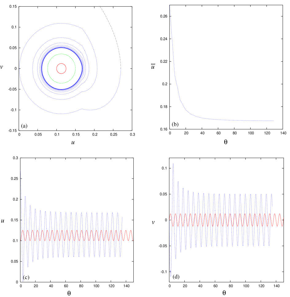
Figure 5: The result for $M_{b}=0.1$ and $k_{2}=0.1$ with $\alpha=0.1$, $r_{1}=3$, $r_{2}=6$. (a) Solution curves on the $u-v$ phase-plane. (b) $\bar{u}$ as a function of $\theta$, where $\bar{u}$ are the values of $u$ of the blue dotted curve in (a) and satisfied $u>0.12$ and $v=0$. (c) The plots of $u$ as a function of $\theta$. (d) The plots of $v$ as a function of $\theta$. The red solid (blue dotted) curves in all panels correspond to the same solution.

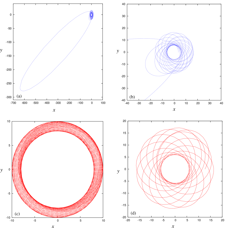
Figure 6: The result for $M_{b}=0.1$ and $k_{2}=0.1$ with $\alpha=0.1$, $r_{1}=3$, $r_{2}=6$. (a) The orbit on the $x-y$ plane for the blue dotted curve in Figure 5(a). (b) The closer view of (a). (c) The orbit on the $x-y$ plane for the red solid curve in Figure 5(a). (d) Another orbit for arbitrary given solution curve approaching the limit cycle.

Figures 5-6 are for the case when we set $M_{b}=0.1$ and $k_{2}=0.1$. We assume the frictional parameter $\alpha=0.1$ for this case. We know from Figure 1, that there is only one fixed point and Figure 5(a) shows that this fixed point is a center point. We found that there is a “limit cycle” that all solution curves out of this cycle are approaching this cycle. However, all the solution curves within this cycle do not, they still behave as normal curves around a center point. Therefore, this kind of “limit cycle” is called a “semi-attractor”.

To understand how these outer solution curves approach this “limit cycle”, we simply pick up the blue dotted curve’s representative points which are on the right hand side of the fixed point and cross $v=0$ line, i.e. the points satisfying $u>0.12$ and $v=0$ in Figure 5(a). Figure 5(b) is the plot of the $u$ values of these points, $\bar{u}$, as a function of $\theta$ when we set initial $\theta=0$. We can see that $\bar{u}$ approaches to ${\bar{u}}=1/r_{2}=1/6$ and the approaching speed decays very quickly. In Figure 5(b), we see that the curve almost becomes a straight line, i.e. $d{\bar{u}}/d{\theta}=0$ when $\theta>100$.

The blue dotted curves in Figure 5(c)-(d) show $u$ and $v$ as functions of $\theta$ and the curve in Figure 6(a) shows the orbit on the $x-y$ plane for the above solution curve which approaches the “limit cycle”. Figure 6(b) is the closer view of Figure 6(a).

Moreover, the red solid curves in Figure 5(c)-(d) show the $u$ and $v$ as function of $\theta$ and the curve in Figure 6(c) shows the orbit on the $x-y$ plane for the red solid solution curve around the center point in Figure 5(a).

Figure 6(d) is another orbit for a given solution curve approaching the “limit cycle”. The orbit is getting closer to a precessing ellipse when the solution curve approaches the “limit cycle” as we can see in both Figure 6(b) and Figure 6(d).

5 Conclusions

We have studied the orbital evolution and also stability of planetary systems with interaction from belts by the standard phase-plane analysis. We regard the mass of the belt $M_{b}$ and $k_{2}$ ($=m^{2}/l^{2}$) as the two main parameters to determine the location of fixed points and also classify the outcome of orbital evolution. Please note that the fixed points on the phase space corresponds to the circular orbits on the orbital plane.

From the results in Figure 1, we know that when the belt’s mass is small, the bifurcation diagram is almost a straight line, i.e. Keplerian orbits. When the belt’s mass is larger, there could be more than one fixed point, one still corresponding to the Keplerian orbit and the new fixed points always close to the inner edge $u=1/r_{1}$ or outer edge $u=1/r_{2}$ of the belt.

However, since the needle-like structure around the outer edge in Figure 1 is very tiny, the probability that the planet moves stably around the outer edge is much smaller than near the inner edge. This conclusion is consistent with the principle result in Jiang & Yeh [2003].

There is one interesting case in which we found a limit cycle of semi-attractor type: the solution curves lying outside of the cycle approach this cycle but the ones within this cycle do not. In this case, the orbit is getting similar to a precessing ellipse when the solution curve approaches the limit cycle.

What could we learn for the Solar System from these theoretical results ?

It is known that there is a belt, the Kuiper Belt, in the outer Solar System after the first Kuiper Belt Object (KBO) was detected (Jewitt & Luu [1993]). Many more KBOs have been detected since then and now there are more than 500 discovered KBOs. Allen, Bernstein & Malhotra [2001] did a survey and found that they could not find any KBOs larger than 160 km in diameter beyond 50 AU in the outer solar system. They suggested several possible explanations for this observational result.

If we apply our model to this problem, the point mass which represents the planet in our model, now represents a KBO. Our results imply that the big KBOs would have greater probability of approaching the inner edge of the Kuiper Belt and the small KBOs would not. This is because the value of $k_{2}$ would be larger when $m$ is large for a given initial angular momentum, and thus it corresponds to the right branch of curves in Figure 1. If $m$ is much smaller and $k_{2}<0.1$, it corresponds to the left branch of curves in Figure 1 and thus the small KBOs might not approach the inner edge of the Kuiper Belt.

Therefore, our result is consistent with one of the possible reasons: larger KBOs might have been displaced to their present orbits by a large-scale rearrangement of orbit (Allen, Bernstein & Malhotra [2001]). In fact, our results provide a natural mechanism to do this orbit rearrangement: larger KBOs might have been moving towards the inner edge of the belt due to the friction from the belt.

Appendix A Gravitational Force from the Belt $f_{b}$

Let $F(\xi)$ be an elliptic integral of the first kind and assume

$$\xi=\frac{2\sqrt{rr^{\prime}}}{r+r^{\prime}}.$$ (A1)

By $\sin^{2}A=\frac{1}{2}(1-\cos 2A)$, we have

$$F(\xi)=\int^{\pi/2}_{0}\frac{1}{\sqrt{1-\xi^{2}\sin^{2}\phi^{\prime}}}d\phi^{\prime}=\frac{(r+r^{\prime})}{2}\int^{\pi}_{0}\frac{1}{\sqrt{r^{2}+r^{\prime 2}-2rr^{\prime}\cos(\phi)}}d\phi.$$ (A2)

Therefore, from Equation (A2), we have

$$\int^{2\pi}_{0}\frac{1}{\sqrt{r^{2}+r^{\prime 2}-2rr^{\prime}\cos(\phi)}}d\phi=2\int^{\pi}_{0}\frac{1}{\sqrt{r^{2}+r^{\prime 2}-2rr^{\prime}\cos(\phi)}}d\phi=\frac{4F(\xi)}{r+r^{\prime}}.$$ (A3)

The gravitational potential is

$$V(r)=-G\int^{r_{2}}_{r_{1}}\!\int^{2\pi}_{0}\frac{\rho(r^{\prime})r^{\prime}}{\sqrt{r^{2}+r^{\prime 2}-2rr^{\prime}\cos(\phi^{\prime})}}dr^{\prime}\!d\phi^{\prime}=-4G\int^{r_{2}}_{r_{1}}\frac{F(\xi)\rho(r^{\prime})r^{\prime}}{r+r^{\prime}}dr^{\prime},$$ (A4)

where Equation (A3) has been used.

Now we differentiate this potential with respect to $r$ to get the gravitational force, so

$$f_{b}=-\frac{\partial V}{\partial r}=4G\int^{r_{2}}_{r_{1}}\frac{\frac{dF(\xi)}{d\xi}\frac{\partial\xi}{\partial r}\rho^{\prime}(r^{\prime})r^{\prime}}{r+r^{\prime}}dr^{\prime}+4G\int^{r_{2}}_{r_{1}}F(\xi)\rho(r^{\prime})r^{\prime}\frac{\partial}{\partial r}\left(\frac{1}{r+r^{\prime}}\right)dr^{\prime}.$$ (A5)

Let $E(\xi)$ be an elliptic integral of the second kind and $\xi^{\prime}=\sqrt{1-\xi^{2}}$. Since $F(\xi)$ is an elliptic integral of the first kind, from Byrd & Friedman [1971], we have

$$\frac{dF(\xi)}{d\xi}=\frac{E-\xi^{\prime 2}F(\xi)}{\xi\xi^{\prime 2}}=\frac{E}{\xi(1-\xi^{2})}-\frac{F}{\xi}.$$ (A6)

By Equation (A1) and (A6), we calculate

$$\frac{dF(\xi)}{d\xi}\frac{\partial\xi}{\partial r}=\left[\frac{E}{\xi(1-\xi^{2})}-\frac{F}{\xi}\right]\sqrt{\frac{r^{\prime}}{r}}\frac{r^{\prime}-r}{(r+r^{\prime})^{2}}=-\frac{E(r+r^{\prime})}{2r(r-r^{\prime})}+\frac{F(r-r^{\prime})}{2r(r+r^{\prime})}.$$ (A7)

We substitute Equation (A7) into Equation (A5), so we have

$$f_{b}=-\frac{\partial V}{\partial r}=-2G\int^{r_{2}}_{r_{1}}\frac{\rho(r^{\prime})r^{\prime}}{r}\left[\frac{1}{r-r^{\prime}}E+\frac{1}{r+r^{\prime}}F\right]dr^{\prime}.$$ (A8)

If the planet is on the belt region, there is a singularity for $f_{b}$ and we introduce a small $\epsilon>0$ to avoid it. That is, we numerically calculate the force from the belt by the following formula:

$$f_{b}=-2G\int^{r-\epsilon}_{r_{1}}\frac{\rho(r^{\prime})r^{\prime}}{r}\left[\frac{1}{r-r^{\prime}}E+\frac{1}{r+r^{\prime}}F\right]dr^{\prime}-2G\int^{r_{2}}_{r+\epsilon}\frac{\rho(r^{\prime})r^{\prime}}{r}\left[\frac{1}{r-r^{\prime}}E+\frac{1}{r+r^{\prime}}F\right]dr^{\prime}.$$ (A9)

Similar treatment can be done for the integrals in Appendix B.

Appendix B Derivatives of $f_{b}$

From Equation (A8), we calculate

$$\frac{\partial f_{b}(r)}{\partial r} = \frac{2G}{r^{2}}\int^{r_{2}}_{r_{1}}r^{\prime}\rho(r^{\prime})\left[\frac{1}{r-r^{\prime}}E+\frac{1}{r+r^{\prime}}F\right]dr^{\prime}$$ (B1)

$$-\frac{2G}{r}\int^{r_{2}}_{r_{1}}r^{\prime}\rho(r^{\prime})\left[\frac{\frac{dE}{d\xi}\frac{d\xi}{dr}}{r-r^{\prime}}+E\frac{d}{dr}\left(\frac{1}{r-r^{\prime}}\right)+\frac{\frac{dF}{d\xi}\frac{d\xi}{dr}}{r+r^{\prime}}+F\frac{d}{dr}\left(\frac{1}{r+r^{\prime}}\right)\right]dr^{\prime}.$$

From Byrd & Friedman (1971),

$$\frac{dE}{d\xi}=\frac{1}{\xi}(E-F)=\frac{r+r^{\prime}}{2\sqrt{rr^{\prime}}}(E-F).$$

Thus,

$$\frac{dE}{d\xi}\frac{d\xi}{dr}=\frac{r^{\prime}-r}{2r(r+r^{\prime})}(E-F).$$ (B2)

We substitute Equation (A7) and Equation (B2) into Equation (B1), so we have

$$\frac{\partial f_{b}(r)}{\partial r}=\frac{2G}{r^{2}}\int^{r_{2}}_{r_{1}}r^{\prime}\rho(r^{\prime})\left\{\frac{3r^{2}-r^{\prime 2}}{(r-r^{\prime})^{2}(r+r^{\prime})}E+\frac{1}{r+r^{\prime}}F\right\}dr^{\prime}.$$ (B3)

Hence, from Equation (A8), we have

$$\frac{1}{u^{4}}\frac{\partial f}{\partial r}+\frac{2f_{b}}{u^{3}}=\frac{2G}{u}\int^{r_{2}}_{r_{1}}r^{\prime}\rho(r^{\prime})\left\{\frac{1+r^{\prime 2}u^{2}}{(1-r^{\prime}u)^{2}(1+r^{\prime}u)}E-\frac{1}{1+r^{\prime}u}F\right\}dr^{\prime}.$$ (B4)

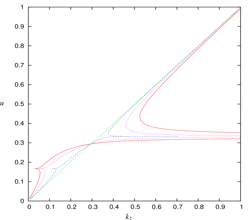
Figure 1: The bifurcation diagram of fixed points on the $k_{2}-u$ plane with $r_{1}=3$, $r_{2}=6$, where the green dashed curves are for $M_{b}=0.01$, the blue dotted curves are for $M_{b}=0.1$, the purple dotted curves are for $M_{b}=0.5$ and the red solid curves are for $M_{b}=1$.

References

- (1) Allen, R. L., Bernstein, G. M., Malhotra, R. [2001] “The edge of the Solar System”, The Astrophysical Journal, 549, 241-244.
- (2) Byrd, P. F., Friedman, M. D. [1971] “Handbook of elliptic integrals for engineers and scientists”, 2nd Edition, Springer-Verlag.
- (3) Clausen, S., Helgesen, G., Skjeltorp, A.T. [1998] “Braid description of few body dynamics”, Int. J. Bifurcation and Chaos 7, 1383-1397.
- (4) Goldstein, H. [1980] “Classical mechanics”, Addison-Wesley Publishing Company.
- (5) Jayawardhana, R., Holland, W. S., Greaves, J. S., Dent, W. R. F., Marcy, G. W., Hartmann, L. W., Fazio, G. G. [2000] “Dust in the 55 Cancri planetary system”, The Astrophysical Journal, 536, 425-428.
- (6) Jewitt, D., Luu, J. X. [1993] “Discovery of the candidate Kuiper Belt object 1992 QB”, Nature, 362, 730-732
- (7) Jiang, I.-G., Ip, W.-H. [2001] “The planetary system of upsilon Andromedae”, Astron. & Astrophys., 367, 943-948.
- (8) Jiang, I.-G., Yeh, L.-C. [2003] “Bifurcation for dynamical systems of planet-belt interaction”, Int. J. Bifurcation and Chaos, 13, 534.
- (9) Kaulakys, B., Ivanauskas, F., Meskauskas, T. [1999] “Synchronization of chaotic systems driven by identical noise”, Int. J. Bifurcation and Chaos 9, 533-539.
- (10) Lizano, S., Shu, F. H. [1989] “Molecular cloud cores and bimodal star formation”, The Astrophysical Journal, 342, 834-854.
- (11) Marcy, G. W., Butler, R. P., Fischer, D. A., Laughlin, G., Vogt, S. S., Henry, G. W., Pourbaix, D. [2002] “A planet at 5 AU around 55 Cancri”, The Astrophysical Journal, 581, 1375-1388.
- (12) Marcy, G. W., Butler, R. P., Williams, E., Bildsten, L., Graham, J. R., Ghez, A. M., Jernigan, J. G. [1997] “The planet around 51 Pegasi”, The Astrophysical Journal, 481, 926-935.
- (13) Murray, C. D., Dermott, S. F. [1999] “Solar system dynamics”, Cambridge University Press.
- (14) Terquem, C., Papaloizou, J. C. B. [2002] “Dynamical relaxation and the orbits of low-mass extrasolar planets”, Monthly Notices of the Royal Astronomical Society, 332, 39-43.
- (15) Thommes, E.W., Duncan, M.J., Levison, H.F. [1999] “The formation of Uranus and Neptune in the Jupiter-Saturn region of the Solar System”, Nature, 402, 635-638.
- (16) Xia, Z. [1993] “Arnold diffusion in the elliptic restricted three-body problem”, J. Dynam. Differential Equations 5, 219-240.
- (17) Yeh, L.-C., Jiang, I.-G. [2001] “Orbital evolution of scattered planets”, The Astrophysical Journal 561, 364-371.