Scattered Light from Close-in Extrasolar Planets:
Prospects of Detection with the MOST Satellite

Abstract

The ultra-precise photometric space satellite MOST (Microvariability and Oscillations of STars) will provide the first opportunity to measure the albedos and scattered light curves from known short-period extrasolar planets. Due to the changing phases of an extrasolar planet as it orbits its parent star, the combined light of the planet-star system will vary on the order of tens of micromagnitudes. The amplitude and shape of the resulting light curve is sensitive to the planet’s radius and orbital inclination, as well as the composition and size distribution of the scattering particles in the planet’s atmosphere.

To predict the capabilities of MOST and other planned space missions, we have constructed a series of models of such light curves, improving upon earlier work by incorporating more realistic details such as: limb darkening of the star, intrinsic granulation noise in the star itself, tidal distortion and back-heating, higher angular resolution of the light scattering from the planet, and exploration of the significance of the angular size of the star as seen from the planet. We use photometric performance simulations of the MOST satellite, with the light curve models as inputs, for one of the mission’s primary targets, $\tau$ Boötis. These simulations demonstrate that, even adopting a very conservative signal detection limit of 4.2 $\mu$mag in amplitude (not power), we will be able to either detect the $\tau$ Boötis planet light curve or put severe constraints on possible extrasolar planet atmospheric models.

1 Introduction

Since the discovery of a planet around 51 Peg b in 1995 (Mayor & Queloz 1995), the field of extrasolar planetary research has grown steadily. Radial velocity surveys (e.g., Marcy et al. 2003; Santos et al. 2000; Tinney et al. 2002) have found over 100 extrasolar giant planets (EGPs) orbiting nearby stars. In addition, $\sim$ 10 of these systems contain planets with semi-major axes $\lesssim 0.05$ AU, here after called close-in EGPs (CEGPs). The radial velocity surveys provide the planet’s minimum mass and orbital parameters (such as semi-major axis and eccentricity) but nothing else about the planet’s properties. Despite the growing numbers of discoveries, we only know detailed and accurate properties of a single extrasolar planet: HD 209458b. Observations of this transiting planet HD 209458b (Charbonneau et al. 2000; Henry et al. 2000; Brown et al. 2001) have provided measurements of the radius and mean density of the planet, providing the first information on the planet’s composition. Furthermore, the detection of the trace element sodium in HD209458b’s atmosphere by Charbonneau et al. (2002) has provided the first constraint on an extrasolar planet’s atmosphere.

Ongoing planet transit searches (see Horne 2003) should increase the number of extrasolar planets with observed physical properties by providing a measured radius and inclination for discovered planets—see Konacki et al. (2003) for a description of the first planet detected with the transit search method. However, even for transits, little information is coming directly from the planet. For non-transiting planets, direct spectroscopy and photometry appear to be the most likely sources of additional information. Spectroscopy could reveal atmospheric composition. Ultra-precise photometry has the potential to reveal the nature of the atmospheric scattering particles: due to the changing phases of a short-period extrasolar planet as it orbits its parent star, the combined light of the planet-star system will vary on the order of tens of micromagnitudes. The shape of the resulting light curve is indicative of the atmospheric scattering particles’ composition and size distribution. Unfortunately, ground-based photometry is limited by atmospheric scintillation to detect magnitude variations of $10^{-4}$. Such precision is generally only possible for bright variable stars with periods of only a few minutes, such as the rapidly oscillating Ap (roAp) stars, where long-term drifts do not interfere with signal detection at high frequencies. An example of the state of the art in rapid ground-based photometry is the work of Kurtz et al. (2003), who set a threshold of 0.2 millimag in their null detection of oscillations in the Ap star HD 965. For periods of days, we know of no photometric measurements that have achieved this level of precision. However, assuming a grey albedo, an upper limit of $5\cdot 10^{-5}$ for the variation of the flux ratio has been establish for the $\tau$ Boötis system (Charbonneau et al. 1999, Leigh et al. 2003). The planetary light curve amplitudes are anticipated to be below this threshold. Nevertheless, planned space-based photometric telescopes are expected to detect $\mu$mag variations in the next few years.

The first of these missions to go into orbit should be MOST (Microvariability and Oscillations of STars)—a Canadian Space Agency microsatellite housing an ultra-precise photometric instrument, to be launched on 30 June 2003. MOST was designed to detect and characterize rapid acoustic oscillations in solar-type stars, but it also has the potential to measure the scattered light from known CEGPs. The light curve data are sensitive to a planet’s radius, inclination, and most importantly albedo, which in turn depends on the thermal equilibrium of the planet and the composition and size range of the primary scattering particles.

MOST will not be searching stars for new planets, due to its small aperture and limited number of accessible targets, but rather monitoring stars already known to have CEGPs, searching for scattered light signals whose periods are already well determined. The goal is to detect the scattered light signature of an extrasolar planet for the first time, and to provide empirical data to test models of CEGP atmospheric composition. The MOST target list includes three stars with CEGPs in its first two years: 51 Peg, $\tau$ Boötis, and HD 209458. The photometric data will also be used to search for solar-type oscillations in the parent stars, whose eigenspectra can better refine their masses and main-sequence ages. This will also be extremely valuable in understanding the nature and history of the CEGPs themselves.

Other funded space missions—COROT (CNES/ESA 2005), Kepler (NASA 2007) and Eddington (ESA 2007)—will monitor fields of tens of thousands of stars, discovering hundreds of new EGPs by their scattered light curves (in addition to their primary extrasolar planet goal of searching for transiting Earth-sized planets). MOST will provide a valuable starting point for these missions by determining the signature of the CEGP light curves that can then be used for detection algorithms and also by characterizing the low-amplitude photometric variability of solar-type stars, which will affect planet light curve and transit detections. A recent paper by Jenkins & Doyle (2003) evaluates Kepler’s ability to discover CEGPs by their light curves, around stars without known planets. Their paper includes an estimate of the number of planets Kepler expects to detect and a description of detection algorithms. Our paper is complementary, describing MOST’s potential for detecting CEGP light curves of known planets with known orbital periods.

Using a Monte Carlo method, Seager, Whitney, & Sasselov (2000) first generated scattered light curves for generic close-in EGPs to show that the resulting light curves were highly dependent on the composition and size distribution of the condensates in the atmosphere. Furthermore, Seager et al. (2000) showed that systems like 51 Peg might show light variations as large as 60 $\mu$mag peak-to-peak. Even signals twenty times smaller are expected to be within the range of detectability by MOST and other space missions, so these early results inspired the MOST team to expand their science mission to include CEGPs.

In this paper, we present the results of physically more complete models of CEGP scattered light curves that include various types of noise, and we evaluate MOST’s capability to detect them. In §2, we describe the planet atmosphere model and the Monte Carlo model used to produce the synthetic planet light curve data. The stellar noise model is described in §3 and the MOST performance simulation in §4. In §5 we present preliminary results and discussion of both the model and the simulated MOST data. We conclude the paper with a discussion of future prospects in §6.

2 The Planet Scattered Light Curve Model

2.1 The Atmosphere Structure Model

The 3D Monte Carlo (MC) model aims to compute the emergent flux at visible wavelengths from starlight that has anisotropically scattered through the planetary atmosphere. In order to compute the photons’ paths through the atmosphere an input atmospheric structure is needed. For the MC code purposes, this input atmospheric structure consists simply of the wavelength-dependent absorption and scattering coefficients as a function of location in the atmosphere. For simplicity we consider a homogeneous atmosphere in which case only a 1D radial profile (i.e., as a function of vertical atmospheric depth) of absorption and scattering coefficients is needed. (The 3D MC code is required because of highly anisotropic scattering properties of some condensate particles.) Computing the radial distribution and abundance of all of the different absorption and scattering coefficients themselves is a complex task and depends on temperature, pressure and chemical abundances, as described below.

2.1.1 Description of The Model Atmosphere

The atmosphere model used here is a 1D plane-parallel radiative + convective equilibrium code. Full details are described in Seager (1999), Seager et al. (2000), and Seager & Sasselov (in preparation). Three parameters that describe the atmosphere are solved from three equations in a Newton-Raphson type scheme. The three parameters are temperature (as a function of depth), pressure (as a function of depth) and the radiation field (as a function of wavelength and depth). The three equations are radiative transfer, radiative + convective equilibrium, and hydrostatic equilibrium. These equations and the three parameters are highly coupled, which is why to compute the temperature-pressure structure we must also simultaneously solve for the radiation field. In order to solve the three atmosphere equations, an upper and lower boundary condition are needed. The upper boundary condition is the flux from the parent star computed with Kurucz model atmospheres (Kurucz 1992) and the lower boundary condition is the flux from the interior of the planet. We assume that the heating from irradiation is instantaneously redistributed around the tidally-locked planet (but cf. §2.1.2).

Beyond the equations and boundary conditions there are several other inputs to the model atmosphere code. These include planet semi-major axis and surface gravity. We adopt solar abundances to provide an easily comparable standard for future models. The choice of abundance value is a smaller uncertainty compared to cloud opacity (see uncertainties described in §2.1.2). In addition we do not know if the origin of Jupiter’s high metallicity also applies to extrasolar planets; therefore a higher than solar metallicity is not a suitable reference point. The number density of gas and solid species comes from a Gibbs free energy chemical equilibrium calculation (described in Seager et al. (2000)) which specifies the species abundance as a function of temperature and pressure. The opacities for H₂O, CH₄, Na, K, and pressure-induced H₂-H₂ and H₂-He and MgSiO₃ are used. Note that H₂O is the most important gas in determining the temperature-pressure structure due to stellar irradiation. Full references for the opacities used are listed in Seager et al. (2000). Note that our more recent work (Seager & Sasselov in preparation) shows that use of more recent opacities results a similar temperature-pressure structure to the one used here (Seager & Sasselov, in preparation), certainly similar enough for the goal of this paper. With a self-consistent solution for the vertical temperature-pressure profile in a plane-parallel atmosphere, the absorption and scattering coefficients used in the Monte Carlo calculations come directly out of the calculation.

2.1.2 Model Uncertainties

Our model is relevant to first order and more than sufficient for this paper’s primary goal of computing signatures of extrasolar planets with real instrumental and stellar noise concerns. Nevertheless we must keep in mind that there are many uncertainties in the model and any specific model can involve many choices for input parameters. Ultimately the MOST data will be able to constrain the large choice of parameter space and help narrow down the uncertainties.

Recent calculations of atmospheric circulation (Guillot & Showman 2002; Showman & Guillot 2002; Cho et al. 2003) have shown that the stellar irradiation acting on a close-in tidally-locked gas giant planet could cause a highly non-uniform temperature distribution with horizontal temperature variations of up to 1000 K. While such atmospheric circulation models are not yet sophisticated enough to generate temperature-pressure profiles and emergent spectra they do indicate a major uncertainty of all current CEGP atmospheric structure models that needs to be addressed in the near future. Even though the scattered light curves depend on the illuminated side only, the atmospheric circulation is still necessary to compute the atmospheric structure consistently.

There are many other uncertainties in the atmospheric models. High-temperature condensates such as MgSiO₃, Al₂O₃, and Fe are stable at the expected CEGP atmosphere temperatures and pressures (see e.g., Seager et al. 2000). These high-temperature condensates form clouds, just as water ice does here on Earth. These clouds present a major complication for EGP modeling because the strong condensate opacity is highly sensitive to the composition and size distribution of particles. The size distribution is determined by a number of physical processes that compete for grain growth and grain destruction, including condensation, coalescence, sublimation, and sedimentation. Two recently developed cloud models (Ackerman & Marley 2001; Cooper et al. 2003) aim to predict particle sizes and are meant to be used consistently in a model atmosphere that determines the temperature, pressure, and radiation field (e.g., Marley et al. 2002). Nevertheless even these cloud models are used in homogeneous layers, not patchy clouds that may exist, and the models still have other uncertainties. We use the results of such computations as a basic guide for our choice of cloud particle size. Other uncertainties are about upper atmosphere processes such as photoionization and photochemistry which could cause small absorptive particles.

2.1.3 The Fiducial Atmosphere Models

We must make choices within the large model atmosphere input parameter space; here we have chosen to work with two fiducial models. Both models have solar abundance. The first model is our cloudy model where we choose a vertically and horizontally homogeneous cloud of MgSiO₃ cloud particles that is two pressure-scale heights thick. Note that even though the cloud parameters are hard-wired, the cloud’s vertical location is self consistently solved for according to the temperature-pressure saturated vapour pressure relation. The condensates are prescribed to have a log-normal particle size distribution having mean radii of 5 $\mu$m and $\sigma=1.5$ $\mu$m. The phase function (i.e., the directional scattering probability) of the condensates is computed with a Mie scattering code (see Figure 1). This silicate cloud model is motivated by considering chemistry models (see Fegley & Lodders 1996) that show MgSiO₃ is likely to form first as the planet cools at the expense of other Mg species. In addition, MgSiO₃ is likely to be the “top” cloud that the stellar photons will reach first. This is because MgSiO₃ is likely to be the lowest-temperature condensate at the relevant CEGP temperatures.

For comparison we use a second fiducial model of a cloud-free planet where the scattering is due to Rayleigh scattering mostly from gaseous H₂. The case of no condensates on the dayside may be realized in some cases of atmospheric circulation where condensates are transported to a much cooler night side where they settle out permanently from the atmosphere (Guillot & Showman 2002). For more details of the temperature-pressure profiles and the corresponding emergent spectra see Seager & Sasselov (in preparation).

2.2 Monte Carlo Model

Our Monte Carlo model is based on the methods presented in Code & Whitney (1995) and Seager et al. (2000). The overall Monte Carlo scattering problem involves following photons that come from a star, enter the planet atmosphere at a given location traveling into a given direction, scatter repeatedly in the planetary atmosphere, and finally exit the planet atmosphere. Essentially, probability distributions are produced for all factors involved in the photon scattering problem (e.g., initial position, distance between interactions, absorption vs. scattering) and are sampled according to

$$\xi=\int_{0}^{a}p(x)dx,$$ (1)

where $\xi$ is a random number between 0 and 1, $p(x)$ is the probability density and $a$ is the output value. The process is repeated for each photon individually. Over 50 million photons were used in each run in order to ensure low statistical error. The final photon counts are normalized to give a ratio of the reflected flux from the planet to the flux from the star (flux ratio). One attractive feature of this method is that since each photon is independent of the last, the algorithm running time is linearly dependent on the number of photons used. Although our code lacks efficient algorithms it is still capable of simulating large numbers of photons in relatively short periods of time.

2.2.1 Initial Photon Properties

Before a photon is scattered for the first time initial characteristics of the photon are determined. The photon wavelength is not calculated exactly, but instead a random number determines which range of wavelengths it falls into according to the blackbody spectrum of the star. The MOST bandpass is close to a box function from 400 nm to 750 nm and we have chosen ten wavelength bins to represent this bandpass (based on the planet atmospheric spectrum generated in §2.1).

The initial coordinates and trajectory of the photon must also be generated. The starting coordinates are produced by generating random $x$, $y$ coordinates on a disk of the same radius as the planet. The EGPs with measurable scattered light curves will have semi-major axes within 0.1 AU; the stellar flux is not plane-parallel and so the initial trajectory of the photon is non-trivial to determine. The initial trajectory of the photon is determined from the probability distribution

$$1=k\int_{0}^{R_{s}}{2\over 5}\pi r\left(2+3\cos\left[\arcsin{r\over R_{s}}\right]\right)dr,$$ (2)

which includes an approximation of solar limb darkening (Carroll & Ostlie 1996). In this equation, $r$ is the radial distance on a disk of radius $R_{s}$ (where $R_{s}$ is the parent star radius), and $k$ is the normalization constant. This distribution only approximates the relative amount of light incident from different directions.

2.2.2 Photon Scattering, Absorption, and Flux

Once the photon enters the atmosphere, it is followed through all scattering processes until it exits the atmosphere or is absorbed by a gas or solid particle. Distances between interactions are calculated separately for all types of events (scattering by gas, scattering by solids, absorption by gas, absorption by solids), and the shortest distance sampled produces an interaction. For scattering events, the new trajectory is determined by sampling the appropriate phase function (see Figure 1 for the phase function of MgSiO₃).

Following these interactions, the same distance calculations are repeated until the photon is absorbed or exits the atmosphere. If absorption occurs, we assume the photon vanishes from the MOST bandpass; absorbed photons will be reemitted at IR wavelengths where the CEGP thermal flux peaks. Although the absorbed photons do affect the heat balance of the planet, this is already taken into account from our atmospheric structure models described in §2.1.1–2.1.3. If the photon escapes the atmosphere, it is binned according to trajectory angle relative to the direction of the parent star ($z$-axis). This binning method assumes symmetry about the $z$-axis; reasonable for a symmetric atmosphere with symmetric illumination.

After the pre-specified number of photons have been sent through the atmosphere, the photon counts are normalized to give the emergent flux. At intervals given by expected integration times for MOST of 1-2.5 minutes, the orbital position is calculated from the eccentricity, inclination, semi-major axis and orientation of the orbit. From the orbital position the phase angle (the star-planet-observer angle; in our case the angle between the $z$-axis and the observer) is calculated. The flux for the phase angle is taken from the binned data and normalized for the current distance.

2.2.3 Planet Tidal Distortion Effects on the Light Curve

Sinusoidal modulations in photometric light curves are observed in binary star systems with tight orbits due to tidal distortion of the stars into ellipsoidal shapes (Von Zeipel 1924; Kitamura & Nakamura 1988). Even short-period (2-day) companions to solar-type primaries can cause a gravitational distortion visible on millimag light curves if the companion mass is at least $\sim$ 0.2 $M_{\odot}$ (Drake 2003). We examine the same effects from a tidally distorted planet, to see if they will affect the scattered light curve at the micromagnitude level, by estimating the distorted length of the planet’s axes under the assumption of an isothermal expansion. Assuming equilibrium and cylindrical symmetry,

$$R_{z}={{\left[\ln\left({{g-2g_{t}}\over{g}}\right)-{{m_{H}gR_{p}}\over{k_{b}T}}\right]{k_{b}T}}\over{m_{H}(g-2g_{t})}},$$ (3)

and

$$R_{x}={{\left[\ln\left({{g+g_{t}}\over{g}}\right)-{{m_{H}gR_{p}}\over{k_{b}T}}\right]{k_{b}T}}\over{m_{H}(g+g_{t})}},$$ (4)

where $R_{z}$ is the radius of the planet in the direction of the star, $R_{x}$ is the perpendicular radius and $R_{p}$ is the initial spherical size of the planet. Furthermore, $g$ is the surface gravity, $m_{H}$ is the mass of hydrogen and $k_{b}T$ is the thermal energy. The tidal acceleration is $g_{t}={GM_{s}R_{p}\over{a^{3}}}$, where $M_{s}$ is the stellar mass, $a$ is the semi-major axis and $G$ is the gravitational constant. Given the phase angle, the relative increase or decrease in intensity is added through geometric optics instead calculating it directly in the Monte Carlo code. This approach is approximate, but given the relatively small size alterations the impact of this assumption should be minimal. From the above equations, we found the tidal distortion to be a $\sim$ 10^-7 effect, well below the $\sim$ 10^-5 light curve signal.

2.2.4 Back Heating

CEGPs are expected to be tidally locked due to tidal interactions between the planet and the star (Goldreich & Soter 1966; Guillot et al. 1996). The stellar atmosphere may also be affected by tidal interactions with the CEGP. Combined with the back scattering of light from the planet, the stellar atmospheres could potentially have a flux hot spot with a rotational variation of the same period as the planet’s rotational period. Although stellar back heating is expected to be a small effect, it could be important because it would share the same period as the planetary light curve.

To investigate the magnitude of the back heating effect we construct an approximate model, based on the results of the Monte Carlo code. From the distance between the planet and the star (it is assumed that only roughly circular orbits will produce the back heating effect) and the angular binning used in the scattering code, several rings on the stellar surface are considered. Each stellar ring is considered to initially radiate energy according to the black body equation $E=A\sigma T_{e}^{4}$, where $A$ is the emissivity, $\sigma$ is the Stefan-Boltzmann constant and $T_{e}$ is the effective temperature. Using the same equation for the total flux emitted by the star, an estimate of the scattered energy is produced from the fraction of the light scattered from the planet back towards the star. Since the star must reach equilibrium between the input and expelled energy at each point on the surface, a ratio of the intensity of flux on each ring to the average can be made. Making the approximation that the flux at the planet is unchanged, we get

$${F_{R}(\theta)\over F_{AVG}}=1+{P(\theta)\over Z}\pi R_{s}^{2}{R_{p}^{2}\over a^{2}}{1\over A_{R}},$$ (5)

where $R_{s}$, $R_{p}$ are the star and planet radius, $a$ is the planet semi-major axis, $Z$ is the total number of photons in the Monte Carlo code, while $P(\theta)$ is the number of photons reflecting into angle $\theta$. $A_{R}$ is the area of the ring of the stellar surface produced by binning at $\theta$, $F_{AVG}$ is the initial flux of the ring and $F_{R}$ is the increased flux due to scattered light. This ratio is calculated for each ring on the stellar surface.

Once the increased stellar flux is calculated, a light curve is produced for each ring using the limb darkening profile of the star. The profile is constructed using an approximation for solar limb darkening (Carroll & Ostlie 1996). This limb darkening approximation has good agreement with measurements averaged over the visible spectrum. The increase in stellar flux is spatially integrated over the stellar disk for each time interval. Because of the small size of the scattered light ratio and $R_{p}^{2}\over a^{2}$, our estimate shows back heating to be a small effect (on the order of 10^-7) compared to the $\sim 10^{-5}$ CEGP light curve.

3 Stellar Granulation Noise

One of the fundamental limiting factors in the spectroscopic detection of extrasolar planets through Doppler shifts is the intrinsic radial velocity noise due to the changing pattern of rising granules at the top of the convection zone. The variation in filling factor and contrast of the granulation pattern is also an important noise source in ultra-precise photometry of solar-type stars.

The level of granulation noise is correlated with chromospheric activity, which in turn depends on stellar rotation rate, surface magnetic activity, as well as depth of the surface convection zone. The sample, selected for Doppler searches for extrasolar planets tend to be chromospherically quiescent, so the targets for MOST photometry will also share that trait. However, granulation noise may still be the dominant noise source, especially at low frequencies.

Granulation noise is non-white, and photometry of the Sun suggests that the noise spectrum has an approximate $1/f$ dependence of amplitude on frequency (e.g., Kjeldsen & Frandsen 1992; Kjeldsen & Bedding 1998).

To simulate this noise source, we generate a grid of frequencies from zero to the Nyquist frequency appropriate to the simulated data sample. These values are inverted to create an array of $1/f$ values, then multiplied by a corresponding array of random numbers (distributed normally about zero with a variance of one) to randomize the amplitudes and phases of the components of the intrinsic noise. An inverse discrete Fourier transform on the resulting array yields a synthetic time series of granulation noise. This time series can then be multiplied by a scaling factor to match the overall level of granulation noise to be introduced.

For the Sun, photometric granulation noise at a frequency of 0.1 mHz is approximately 2 parts per million in integrated optical broadband light (see, e.g., Kjeldsen & Bedding 1998). We have been guided by this in our simulations, since ground based photometry of other solar-type stars does not set useful upper limits on the granulation noise at relevant frequencies.

4 MOST as an Ultraprecise Photometer

MOST is a small optical telescope (aperture = 15 cm; Maksutov design), with a single broadband filter ($350\leq\lambda\leq 700$ nm), feeding a CCD photometer, aboard a microsatellite platform (mass = 54 kg; dimensions $60\times 60\times 25$ cm). The microsat will be stabilized to a pointing accuracy of about $\pm 10$ arcsec by a set of miniature low-power reaction wheels designed and built by Dynacon Enterprises Ltd. of Toronto, Canada. Although this level of attitude control outperforms (by a factor of several hundred) any existing microsat with such small inertia, it is still relatively poor pointing for an astronomical instrument. Hence, the MOST photometer is equipped with an array of Fabry microlenses to project fixed images of the entrance pupil of the telescope, illuminated by the target starlight, onto the Science CCD. Unlike a wandering image of the star, this extended Fabry image (covering about 1400 pixels) of the CCD makes the collected signal quite insensitive to the flatfield sensitivity gradients of the detector, even at the sub-pixel scale. For more details about technical aspects of the MOST experiment, see Walker, Matthews et al. (2003).

MOST will be launched into a low-altitude (820 km) circular polar orbit, whose slight inclination will cause it to precess at the sidereal rate, so the orbital plane is synchronous with the Sun. Launch is scheduled for 30 June 2003 aboard a Russian three-stage “Rockot” launch vehicle (designated an SS-19 in the West, since it is a former Soviet ICBM) from the Plesetsk Cosmodrome. It will be injected into an orbit which will keep it above the Earth’s terminator. From this vantage point, the telescope will always look over the shadowed limb of the Earth, minimizing scattered Earthlight which could interfere with the ultraprecise photometry. This orbit also provides a Continuous Viewing Zone (CVZ) in the sky spanning declinations $+34^{\circ}\leq\delta\leq-18^{\circ}$. Stars passing through the centre of this band will remain visible continuously for about 8 weeks. The MOST CVZ includes several prominent extrasolar planet systems, including 51 Pegasi, $\tau$ Boötis, and HD209458, which have been included as primary science targets for the MOST mission.

MOST was designed to achieve the mission’s primary goal of detecting rapid photometric oscillations (periods of several minutes) in bright ($V\leq 6$) solar-type, metal-poor subdwarf and magnetic Ap stars with precisions approaching 1 part per million (1 $\mu$mag). Although MOST is a non-differential photometer, the relatively high frequencies of the periodic oscillations can be clearly distinguished in a Fourier spectrum of the data from the lower-frequency modulations, drifts and noise (e.g., orbital variations with $P_{\rm orb}\simeq 100$ min; granulation noise in the stars themselves).

This is not true for the periodic reflected light signals from extrasolar planets, whose orbital frequencies ($\nu_{\rm orbit}\simeq 0.2-0.3$ d^-1 $\simeq 0.003$ mHz) are very low compared to the intended sensitivity range of MOST ($\nu_{\rm osc}\simeq 0.5-6$ mHz). Therefore, MOST non-differential photometry of extrasolar planet systems will be more prone to the long-term drifts and modulations. If MOST were intended to be a planet hunter, searching this low-frequency regime for unknown periodic signals in a noisy background, this might be a fatal flaw. However, as a probe of known extrasolar planet systems whose periods have already been specified accurately from radial velocity data, MOST can be quite effective, as we will demonstrate in §5.

4.1 Modeling the Photometric Performance of MOST

MOST is optimized to collect very precise photometry for stars in the magnitude range $0.0\leq V\leq 6.0$, with integration times from about 0.2 sec to 60 sec depending on the flux of the target. For extrasolar planet photometry, the integration time would be set to bring the total signal per exposure to about 80% of the full-well potential of each CCD pixel, maximizing S/N without sacrificing linearity. For a star of magnitude $V=0$, MOST would collect approximately $1.6\times 10{{}^{8}}$ electrons/sec, although to avoid saturation on such a bright target, the integration time would have to be about 0.2 sec. For extrasolar planet targets with long periods (compared to the rapid stellar oscillations), fast time sampling is not a consideration so every exposure can be long enough to guarantee a maximum S/N of about 220 per pixel per exposure; hence, a S/N of about 8300 over the entire 1400-pixel Fabry image. Further improvements in S/N are possible by substantially binning these short exposures. With extrasolar planet orbital periods of several days, 60-sec exposures can safely be binned in groups of several hundred without appreciably losing resolution in orbital phase.

As part of the design and testing process for the MOST mission, a comprehensive simulator of MOST photometry was developed, written in IDL (Kuschnig et al. 2003). This simulation code was designed to include as many noise, drift and modulation effects as could be anticipated and modeled by the MOST Instrument and Science Teams. The effects can be grouped into four categories: (1) intrinsic variations and noise from the target star (and planet); (2) orbit and radiation environment; (3) sky background and attitude control errors; and (4) detector and electronics. These will be discussed in more detail by Kuschnig et al. (2003) but are summarized in the next few paragraphs.

1. Effects intrinsic to the target star + planet. These include the Poisson noise associated with the total flux from the system, photometric noise associated with granulation in the star’s photosphere, rotational modulation due to starspots, and the periodic variations in scattered light from the planet. The last three are included in the extrasolar planet light curve model (see §2), although they can also be introduced by the MOST photometry simulator independently.

2. Orbit and radiation environment. MOST will circle the Earth approximately every 100 minutes; the exact period will be known very accurately after launch and final orbital injection. Although from its vantage point above the terminator, MOST will only see the nightside limb of the Earth in normal operation, it is possible that there will be some contamination due to stray light scattered from the Earth, varying with MOST’s orbital period. It is possible to add stray light at a level consistent with albedo models of the Earth (e.g., Shaw et al. 1998; Buzasi 2002). The fluxes of high-energy protons and electrons have been calculated for the MOST orbit, and cosmic ray hits onto the Science CCD based on these fluxes have been included in the simulations. Also, MOST will pass through the South Atlantic Anomaly (SAA), exposing it to much higher particle fluxes for several minutes on some orbits. Rather than try to extract photometry from the CCD during these brief passages, we have conservatively not included these data in the time series, introducing short non-periodic gaps which have only a modest effect on the window function of the Fourier spectrum. The CCDs are temperature stabilized by a passive thermal control system which maintains the operating temperature at about $-40.0\pm 0.1$ C. However, we have anticipated there might be a subtle modulation in temperature of 0.1 C (the level of control of the CCD thermal control system) at the MOST orbit period, and have included that effect on the CCD output.

3. Sky background and attitude control errors. The MOST photometry is obtained through a diaphragm 1 arcminute in diameter, which will include a sky background of Zodiacal light, atomic oxygen glow (even at 820 km altitude), stray Earthlight (already modeled in category (2)), scattered light from off-axis sources, and faint stars and galaxies adjacent to the target in the sky. The MOST Telescope and Camera are equipped with a series of baffles designed to reduce parasitic stray light by a factor of $10^{-12}$, but we conservatively include a variable sky background. Wander in telescope pointing due to attitude control errors of about $\pm 10$ arcsec has several effects: (a) The target starlight beam wanders across the surface of the Fabry lens which produces the pupil image, subtly changing the ray paths within the glass and possibly encountering contaminants on different parts of the lens surface. (b) Faint stars or galaxies near the edge of the diaphragm can wander in and out of the field, varying the sky background level. (c) The pupil image will not be completely fixed, although the image motion will only be at a level of about 0.1 pixel in the MOST focal plane. The attitude control system (ACS) errors are modeled based on simulations of the satellite pointing performance. These models are used to introduce errors due to the target starbeam wander (effect (a)). Effect (b) is negligible for the bright targets we consider here, unless a background star is within about 8 magnitudes of the target star brightness. We have investigated all the target fields – including the extrasolar planet fields – and there are no potentially worrisome neighbours in any field. Effect (c) is negligible because of the large size of the pupil image on the CCD, so even sub-pixel sensitivity variations of a few $\times 10\%$ do not manifest themselves in the pupil image motion.

4. Detector and electronics. These effects include: (a) CCD readout noise; (b) dark noise and possible drifts in dark current; (c) pixel-to-pixel and sub-pixel sensitivity gradients (see (3) above); (d) analogue-to-digital conversion (ADC) non-linearities; (e) slight variations in readout-channel gain; and (f) uncertainties in the integration times.

In our simulations, by far the dominant sources of noise are Poisson statistics (photon noise) and stellar granulation. The photon noise in the $\tau$ Boötis simulations shown in §5 is at a level of 0.74 ppm (1$\sigma$). If granulation noise is included in the simulations, the 1-$\sigma$ noise rises to 1.40 ppm. The other noise sources turn out to be negligible for the timescales associated with CEGP scattered light curves. However, for a more detailed breakdown of the photometric error budget of MOST, see Tables 5 and 6 in Walker, Matthews et al. (2003).

5 Results

5.1 Simulations of Scattered Light Curves

One of the most important aspects of our model is taking into account the angular size of the star as seen from the planet. We have found that using an extended source with limb darkening, the shape of the resulting light curve is significantly altered (see Figure 2) compared to a point source. With a point source, the detailed, high angular resolution features of the phase function of scatterers remain apparent at planet-star separations $\gtrsim$ 0.07 AU. This effect had gone unnoticed in previous simulations (Seager et al. 2000) because of the low angular resolution used to calculate the fluxes scattered from the planet in those models. Our work has shown it is essential to use angular bins of less than a degree to properly compute the light curves, especially for the very close-in extrasolar planets. With the proper source geometry, these features are smoothed for separations smaller than 0.07 AU and the amplitude of the light curve is reduced by up to 20% for orbital inclinations near $90^{\circ}$ (as noted in Seager et al. 2000).

The addition of stellar back heating was found to be negligible even for space-based photometry of precision 1 ppm. Typically, stellar back heating contributed a flux ratio of $10^{-7}$ or less. The effect of tidal distortion was slightly larger than back heating. The tidal distortion alone can change the scattered flux of a planet at 0.045 AU from 0.9956 at minimum projected area to 1.0022 at maximum area, where 1.0 is the undistorted value. This translates to an additional variation of $5\times 10^{-7}$ about the mean in the light curve. Although treatment of both these effects was approximate, our initial estimates suggest that their influences will not be detectable in MOST observations of extrasolar planets. However, they could be important diagnostics in data from later space missions like Kepler and Eddington with improved sensitivity and long-term stability. Therefore, we have retained these effects in our models.

Given that the orbital inclinations, radii and atmospheric structure and compositions are unknown for most extrasolar planets, it is important to understand how the planet scattered light curve varies with these parameters. Here we explore parameter variation for a fixed atmosphere model. The amplitude of the light curve is highly dependent on the inclination. As shown in Figure 3a, the peak value can drop by up to an order of magnitude when the inclination is changed from 90 to 50 degrees. Seager et al. (2000) have studied this effect, which will be very important when considering possible detection of these light curves. The radius, as one might expect, makes a large contribution to the amplitude of the light curve. Over a small range of possible planetary radii, the amplitude at all points varies proportionally to the radius squared (Figure 3c). By comparing the effects of inclination and radius (Figure 3b and 3c), the shape of the curve is altered in a unique way for each parameter (given a specific atmospheric model). From Figure 2, the inclination clearly distorts the light curve shape while the radius simply scales the amplitude. The overall shape and reflective properties of the planet light curve are highly dependent on the presence of clouds in the atmosphere (Figure 4 and also see §2).

A change in the planet’s semi-major axis would change the amplitude of the scattered light curve by a factor of $1/a^{2}$. However, a different semi-major axis will also change the shape of the light curve (Figure 3b). As the semi-major axis increases, the angular size of the star as viewed from the planet decreases. As a result, beyond 0.07 AU distinct features of the phase function become visible because they are not “washed out” by multi-directional photon trajectories (see Figure 2).

Our model does allow for changes in the incident flux and angular size of the star as seen from the planet in the case of a non-circular orbit. However, modeling the change in the planet atmosphere as a function of its changing temperature in an eccentric orbit is much more complicated. Such temperature variations will also affect the photon wavelength distribution and the level of tidal distortion. However, only close-in extrasolar planet systems with nearly circular orbits have been selected as MOST primary targets so the current assumptions of zero eccentricity are valid.

5.2 Simulations of MOST Photometry of Extrasolar Planets

The outputs of the extrasolar planet light curve model described in §2 and §3 were used as the inputs to the MOST photometric simulation program described in §5.2. The light curve model gives the intrinsic variability of the (star + planet) system as seen from above the Earth’s atmosphere, while the photometric simulation adds realistic noise and variability inherent to the MOST instrument. Three different inclinations of the planet orbit have been considered: $i=33^{\circ}$, $i=67^{\circ}$, and $i\sim 90^{\circ}$ (more accurately, the maximum inclination that does not produce transits, since transits have not been observed in $\tau$ Boötis or 51 Peg).

For this paper, we present synthetic data for one of the prime extrasolar planet targets for the MOST mission: $\tau$ Boötis b. The star $\tau$ Boötis can be observed by MOST for about 50 days without interruption (except for brief passages through the SAA; see §4.1), so the synthetic data set spans this time interval. The integration time for each exposure is 24 seconds.

The reduction of the synthetic data has been fairly simple and conservative, deliberately avoiding any calibrations that could be influenced by our foreknowledge of the input. Mean bias values have been subtracted from all the measurements. Exposures obviously affected by cosmic ray strikes, and those collected during spacecraft passage through the SAA, have been discarded. The synthetic data are then binned to produce a net time sampling of 100 min (the orbital period of MOST) to average out any periodic variations in stray light and temperature due to orbital modulation. In these simulations, we have adopted a granulation noise amplitude and spectrum comparable to the Sun (see §3).

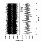
Figure 5: Simulated MOST photometry of $\tau$ Boötis, 67 deg inclination model, time base 50 days. Upper panel: small black squares, signal in [e-] for 25 seconds integrations (data collected in the SAA or affected by cosmic rays have been rejected). Open squares, mean signal [e-] data binned over the spacecraft orbit period of 100 minutes. Lower panel is an expanded view of the binned data.

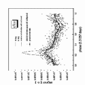
Figure 6: Signals of $\tau$ Boötis model (67^∘ inclination) photometry versus phase of the planet’s orbital period. The open circles represent the binned data, the connected black circles are the mean photometric signals for each (0.05) phase interval. The light curve for the 3 models are shown as well: the dotted line is for 33^∘, the solid line for 67^∘ deg and the dash dot line for the maximum inclination before transit.

The simulated photometry for $\tau$ Boötis observed at an orbital inclination of $i=67^{\circ}$ is presented in Figure 5, showing the unbinned data (filled symbols) and the same data binned into groups of 100 min each (open symbols). The modulation of the flux due to the extrasolar planet orbit orbital period is just barely discernible by eye in the data presented in this form. The periodic modulation becomes more obvious in Figure 6, where those data have been binned in phase according to the known orbital period of $\tau$ Boötis b. Also shown in this figure are the original input models for the three different inclinations modeled. The binned data clearly follow the input model appropriate for this data set.

5.3 Harmonic Structure of the Light Curves

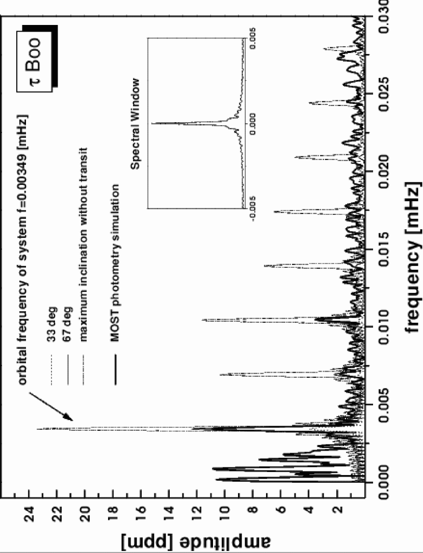
Figure 7: Amplitude spectra a) of a $\tau$ Boötis model (67^∘ inclination), b) photon, instrumental and granulation noise, c) combined. In addition the spectral window is shown (upper panel). The Fourier analysis of the noise has been applied to the binned data with a time base of 50 days.

The detection and characterization of the planet scattered light variation is even more obvious in Fourier space. In Figure 7 we show Fourier amplitude spectra of the time series presented in Figures 5 and 6, plotted out to a frequency of 0.03 mHz. The Nyquist frequency of the sample is 0.08 mHz, but there are neither spectral window artifacts nor increased noise at higher frequencies. The inset in Figure 7 shows the spectral window function, demonstrating that the MOST data sampling does not introduce any serious aliasing. These data contain intrinsic stellar granulation noise with a 1/f frequency dependence, which is principally evident starting at frequencies below 0.003 mHz.

The fundamental peak and characteristic harmonics in Fourier space make even the low-amplitude periodic signals easier to recognize. However, Figure 7 also shows that the Fourier spectrum of the photometry is a valuable way to objectively describe the detailed shape of the light curve. The spectrum of the simulated MOST data is plotted as the bold curve, while the three representative input simulations of the planet light curves are lighter lines. The MOST “data” and the $67^{\circ}$-inclination model to which it corresponds lie on top of one another. Note also that the harmonic structure of the light curves is very sensitive to the inclination. The amplitude ratio of the first harmonic to fundamental drops noticeably with decreasing inclination compared to higher harmonics.

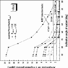
Figure 8: Amplitude of the five highest Fourier peaks as a function of orbital inclination (corresponding to the fundamental and the four lowest harmonics relative to the fundamental) for the $\tau$ Boötis amplitude spectrum shown in Figure 7. The horizontal lines (from bottom to top) show the mean noise level, and the 2$\sigma$ and 3$\sigma$ detection limits. (Note that in the power spectrum, as opposed to this amplitude spectrum, the signal-to-noise will be squared.)

To investigate this further, we generated a more complete grid of models sampling orbital inclination $i$, for two planet radii (1.1 and 1.5 Jupiter radii), and plotted the fundamental and harmonic peak amplitudes as a function of orbital inclination $i$ (Figure 8). This figure also quantifies our ability to detect light variations for various inclinations and radii (for our fixed fiducial model atmosphere). We show in Figure 8 a very conservative detection limit of 4.2 ppm; this is $3\times$ the mean noise level, corresponding to about 99.7% confidence. We emphasize that the detection threshold given in Figure 8 is extremely conservative, based on the detection of signal peaks in amplitude (not power) whose frequencies are not known a priori. In a power spectrum, the signal-to-noise evident in Figure 8 would be squared, but we prefer to present amplitude spectra to err on the side of caution. Also, we will know in advance the frequencies of the fundamental orbital period and its harmonics, so the standard $3\sigma$ detection limit is a severe overestimate. Figure 8 suggests that planetary reflected light signals should be detectable even at relatively modest orbital inclinations.

The harmonic amplitudes have different dependences on inclination and radius, which will be valuable in finding the correct match between model and data. The “forward” approach of adjusting the model to fit the observations is not efficient and may lead to close but incorrect matches. By comparing the harmonic content of the data to those of models from a grid of extrasolar planet parameters, we can eliminate obvious mismatches and narrow the search to the most promising candidate models more quickly and reliably. This approach is already widely used in the pulsating star community, where Fourier decomposition of $\delta$ Scuti light curves has become a valuable tool in identifying non-radial modes in those pulsators (e.g., Poretti 2001 and references therein). We are exploring the diagnostic potential of Fourier decomposition for extrasolar planet light curves, including the underlying physics which affect the light curve shapes, and will present this work in a subsequent paper.

6 Discussion and Conclusions

The first detection and measurements (even of moderate S/N) of CEGP light curves will significantly advance our understanding of these planets. MOST will be the first instrument with the photometric precision to tackle this task. To demonstrate MOST’s exciting potential, we have run a series of simulations for a specific fiducial atmospheric model of the planet $\tau$ Boötis b (described in §2). Other atmosphere models will result in different light curve shapes and amplitudes; however, the condensate size distribution we have adopted is plausible for a quiescent atmosphere (Ackerman & Marley 2001; Cooper et al. 2003). The parameter space of CEGP atmospheric unknowns is so large at present (see §2.1.2) that a full exploration is beyond the scope of this initial study. MOST will soon return real data, either measuring the albedo and the CEGP light curve shape, or setting a meaningful upper limit. This will greatly narrow the allowed range of parameter space of atmospheric models.

Using our fiducial model for $\tau$ Boötis b, orbiting with a period of about 3.3 days, we have shown that MOST’s conservative threshold for detection of a light variation is about 2.5 ppm, with binned data taken over 50 days. This estimate includes realistic models of both stellar granulation noise and of MOST’s noise environment. Such a low limit means we have a good chance to measure the planet light curve even if the atmosphere differs from our fiducial model. Furthermore, MOST should detect the CEGPs across a relatively broad range of orbital inclinations. The Fourier amplitude spectrum of the data will be particularly sensitive to the signal and the detailed shape of its light curve.

Because the actual light curve shape (and hence dominant scattering particle type) is unknown a priori, we will need to fit many different atmosphere models with different radii and inclinations to the real data. Although from our simulations we can recover the fiducial input model, including the planet radius and inclination, there is little point specifying the accuracy of such a recovery; with real data the goal is to detect and measure the shape of the light curve to constrain the atmosphere model, radius, and inclination. Although this work indicates that the degeneracy between planet light curve, radius, and inclination should not be severe, more work is needed to explore this for a variety of atmosphere models.

The case of HD 209458b offers a unique opportunity to determine the atmospheric composition because the planet’s radius and inclination are already known from fits to the transit light curve. A measurement of the secondary transit would give the albedo at a known phase angle and radius. In addition the shape of the light curve will aid us in first determining a light curve signature to be used in detection of light curves from planets with non-edge-on inclinations, and in progressing towards a workable model of the atmosphere. We are currently working on simulations of HD 209458b.

In modeling CEGP light curves we have made several improvements and extensions upon previous work. One significant point is that the angular size of the star is important for planets with semi-major axes $<$ 0.1 AU. This affects the high-angular-resolution features of the light curve compared to using a point-source star (see Figure 2). In addition, modeling the light curve with a star of finite angular size instead of a point source causes a reduction in amplitude of a highly backscattering-peaked light curve by approximately 20 percent (as first noted in Seager et al. 2000). The other new effects we investigated, tidal distortion of the planet and stellar backheating, were found to have a negligible effect on the planet light curve at the level of sensitivity of the MOST instrument but may be important for subsequent space missions.

The results of this paper strongly suggest that MOST will be able to detect the $\tau$ Boötis planet light curve. Even a null result on this star and the other CEGP’s in the MOST target list—given the ultrahigh photometric precision attainable—would eliminate a vast range of extrasolar planet atmosphere models with medium to high albedos.

Figure 1: The phase function of MgSiO₃ at at wavelength of 400.6 nm. We use a log-normal particle size distribution with mean radii of 5 $\mu$m and $\sigma=1.5$ $\mu$m. The phase function at other wavelengths used are not shown.

Figure 2: Simulated scattered light curve of $\tau$ Boötis. The flux ratio is given by the ratio between the reflected flux of the planet and flux from the star. The different lines are for different parent star assumptions: a limb darkened sphere with 0.5 degree binning (solid line; the limb darkening is a model consistent with measurements averaged over the visible spectrum), a point source (dashed line) with 0.5 degree binning, and a point source with 6 degree binning in the light curve (dotted line). Note the features in the light curve near time = 1 day when a point source (i.e., plane-parallel light rays) with 0.5 degree binning is used.

Figure 3: Effects of changing the inclination, semi-major axis, and planet radius on the planet light curve for our fiducial model atmosphere. Panel a: effects of inclination on our $\tau$ Boötis model at 0.035 AU and with $R_{p}$ = 1.3 $R_{J}$. The different inclinations shown are: 30 (long dash dot), 50 (short dash dot), 67 (long dash), 75 (short dash), and 80 (dot) degrees as well as the maximum before transit (solid), 85 degrees. Panel b: the effects of changing $R_{p}$ and inclination for a model planet at 0.045 AU. The planet radius is 1.5 $R_{J}$ (top set of curves), 1.2 $R_{J}$ (middle set of curves) and 0.9 $R_{J}$ (bottom set of curves), and inclinations of maximum before transit (solid) and 66 degrees (dot), and 33 degrees (dashed). Note that the planet atmosphere model was not changed to account for the different $R_{p}$. Panel c: effects of different semi-major axes on our $\tau$ Boötis model of 1.3 $R_{J}$ at maximum inclination before transit. The semi-major axes are 0.045 AU (solid), 0.05 AU (dot), 0.06 AU (short dash) and 0.07 AU (long dash). Note that the planet atmosphere model was not changed to account for the different semi-major axes and parent star irradiation.

Figure 4: A model planet at 0.05 AU and $R_{p}$ = 1.3 $R_{J}$ is shown with (solid) and without (dash) a cloud layer.

References

- (1) Ackerman, A. S., & Marley, M. S. 2001, ApJ, 556, 872
- (2) Brown, T., Charbonneau, D., Gilliland, R., Noyes, R. W., & Burrows, A. 2001, ApJ, 552, 699
- (3) Buzasi, D. L, 2000 The Third MONS Workshop: Science Preparation and Target Selection, Proceedings 2000, eds. T.C. Teixeira, and T.R. Bedding, Aarhus Universitet, 2000., p.9
- (4) Carroll, B., & Ostlie,D. 1996, An Introduction to Modern Astrophysics, (Addison-Wesley)
- (5) Charbonneau, D., Brown, T., Noyes, R. W., & Gilliland, R. 2002, ApJ, 568, 377
- (6) Charbonneau, D., Brown, T., Latham, D., & Mayor, M. 2000, ApJ, 529, L45
- (7) Charbonneau, D., Noyes, R. W., Korzennik, S. G., Nisenson, P. Jha, S., Vogt, S. S., & Kibrick, R. I. 1999, ApJ, 522, L145
- (8) Cho, J. Y-K., Menou, K., Hansen, B., & Seager, S. 2002, submitted to ApJ, astro-ph/0209227
- (9) Cooper, C. S., Sudarsky, D., Milsom, J. A., Lunine, J. I., & Burrows, A. 2003, ApJ, in press, astro-ph/0205192
- (10) Code, A., & Whitney B. 1995, ApJ, 441, 400
- (11) Drake, A. J. 2003, submitted to ApJ, astro-ph/0301295
- (12) Fegley, B., & Lodders, K. 1996, ApJ, 472, L37
- (13) Goldreich, P., & Soter, S. 1966, Icarus, 5, 375
- (14) Guillot, T., & Showman, A. 2002, A & A, 385, 156
- (15) Guillot, T., Burrows, A., Hubbard, W. B., Lunine, J. I., & Saumon, D. 1996, ApJ, 459, L35
- (16) Henry, G., Marcy, G., Butler, P., & Vogt, S. 2000, ApJ, 529, L41
- (17) Horne, K. 2003, in Scientific Frontiers in Research on Extrasolar Planets, ASP Conf. Ser., eds. D. Deming and S. Seager, in press
- (18) Jenkins, J. M. & Doyle, L. R. 2003, ApJ, in press, astro-ph/0305473
- (19) Kitamura, M., & Nakamura, Y. 1988, Ap&SS, 145, 117
- (20) Kjeldsen, H. & Bedding, T. 1998, in Proceedings of the First MONS Workshop,(Aarhus Universitet), p. 1
- (21) Kjeldsen, H. & Frandsen, S. 1992, PASP, 104, 413
- (22) Konacki, M., Torres, G., Jha, S., & Sasselov, D. 2003, Nature, 421, 507
- (23) Kurtz, D.W., Dolez, N. and Chevreton, M. 2003. A&A 398, 1117
- (24) Kurucz, R. 1992, in IAU Symp. 159, Stellar Population of Galaxies, ed. B. Barbuy & A. Renzini (Dorderecht: Kluwer), 225
- (25) Kuschnig, R., Matthews, J., Lanting, T., & Walker G., 2003, in preparation
- (26) Leigh, C., Collier Cameron, A., Horne, K., Penny, A., & D. James 2003, astro-ph/0308413
- (27) Marcy, G., Butler, P., Fisher, D., & Vogt, S. 2003, in Scientific Frontiers in Research on Extrasolar Planets, ASP Conf. Ser., eds. D. Deming and S. Seager, in press
- (28) Marley, M. S., Seager, S., Saumon, D., Lodders, K., Ackerman, A. S., Freedman, R. S., & Fan, X. 2002, ApJ, 335
- (29) Poretti, E. 2001, A&A, 371, 986
- (30) Mayor, M., & Queloz, D. 1995, Nature, 378, 355
- (31) Santos N.C. , Mayor M. , Naef D., Pepe F. , Queloz D., Udry S., & Blecha A. 2000, A & A, 361, 265
- (32) Shaw, D., Merle R. and Wilson J., Instrument Science Report STIS 98-21 ”Scattered Light from the Earth Limb Measured with the STIS CCD”
- (33) Showman, A.,& Guillot, T. 2002, A & A, 385, 166
- (34) Seager, S. 1999, PhD Thesis, Harvard University
- (35) Seager, S., Whitney, B., & Sasselov, D. D. 2000, ApJ, 540, 504
- (36) Tinney, C., Butler, P., Marcy, G., Jones, H., Penny, A., McCarthy, C., & Carter, B., 2002, ApJ, 571, 528
- (37) von Zeipel, H. 1924 MNRAS, 84, 665
- (38) Walker, G.A.H., Matthews, J., Kuschnig, R., Johnson, R., Rucinski, S., Pazder, J., and others, 2003, PASP submitted