Extinction Map of the Galactic center: OGLE-II Galactic bulge fields

Abstract

We present the reddening ($E(V-I)$) and Extinction maps in $V$-band ($A_{V}$) and $I$-band ($A_{I}$) for 48 Optical Gravitational Lensing Experiment II (OGLE-II) Galactic bulge (GB) fields, covering a range of $-11^{\circ}<l<11^{\circ}$, with the total area close to 11 square degrees. These measurements are based on two-band photometry of Red Clump Giant (RCG) stars in OGLE-II $VI$ maps of GB. We confirm the anomalous value of the ratio of total to selective extinction $R_{VI}\equiv A_{V}/E(V-I)=1.9\sim 2.1$, depending on the line of sight, as measured by Udalski (2003). By using the average value of $R_{VI}=1.964$ with the standard deviation $sdev=0.085$, we measured $E(V-I)$, $A_{V}$ and $A_{I}$, and we obtained extinction and reddening maps with a high spatial resolution of $26.7^{\prime\prime}\sim 106.8^{\prime\prime}$, depending on the stellar density of each field. We assumed that average, reddening corrected colours of red clump giants are the same in every field. The maps cover the range $0.42<E(V-I)<3.5$, $0.83<A_{V}<6.9$ and $0.41<A_{I}<3.4$ mag respectively. The zero points of these maps are calibrated by using $V-K$ colours of 20 RR Lyrae ab variables (RRab) in Baade’s window. The apparent reddening corrected $I$-band magnitudes of the RCGs change by $+0.4$ mag while the Galactic coordinate $l$ varies from $+5^{\circ}$ to $-5^{\circ}$, indicating that these stars are in the Galactic Bar. The reddening corrected colour of RRab and RCGs in GB are consistent with colours of local stars, while in the past these colours were claimed to be different.

1 Introduction

A study of stellar populations and stellar dynamics in the Galactic Bulge (GB) is important for understanding how bulges formed, what are their populations, gravitational potential and structure.

Several gravitational microlensing survey groups have found hundreds of events towards the Galactic center and disc (EROS: Derue 1999; OGLE: Udalski et al. 2000; Woźniak et al. 2001; MACHO: Alcock et al. 2000; MOA: Bond et al. 2001; Sumi et al. 2003a), and thousands are expected in the upcoming years by MOA , OGLE-III and other collaborations. The data from such microlensing surveys is useful to study the Galactic structure by measuring the microlensing optical depth (Udalski et al. 1994; Alcock et al. 1997, 2000; Sumi et al. 2003a; Afonso et al. 2003; Popowski et al 2003;) and the proper motions of stars (Sumi, Eyer & Woźniak 2003; Sumi et al. 2003b), and well suited for numerous other scientific projects (see Paczyński 1996; Gould 1996).

However, as is well known, the extinction due to the dust is very significant towards the GB. This affects the Color Magnitude Diagram (CMD) of the field and makes a separation of stellar populations difficult. To correct for these effects the measurements of the extinction in these fields are crucial.

Schlegel, Finkbeiner & Davis (1998) made all sky extinction map using COBE/DIRBE data, which overestimate the extinction towards the GB because of background dust (Dutra et al. 2003). Schultheis et al. (1999) and Dutra et al. (2003) constructed $K$-band extinction maps of the Galactic central region with a resolution of $4^{\prime}$ by using $J$ and $K$ photometry of the upper giant branch stars in DENIS and 2MASS data respectively. Some determinations of the extinction towards Baade’s Window have been performed with a number of different techniques, including those of stellar simulation (Ng et al. 1996), mean magnitudes of red-clump stars (Kiraga, Paczyński & Stanek 1997), the absolute magnitude of RR Lyrae stars (Alcock et al. 1998b) and magnitude of the K-giants (Gould, Popowski & Terndrup 1998). The Large-Scale Extinction Map of the Galactic Bulge was made by using the mean colour of all stars in the MACHO Project Photometry (Popowski, Cook & Becker 2003)

Woźniak & Stanek (1996) proposed a method to investigate the ratio of total to selective extinction based on two-band photometry of Red Clump Giants (RCGs). The RCGs are the equivalent of the horizontal branch stars for a metal-rich population, i.e., relatively low-mass core helium burning stars. RCGs in the Galactic bulge occupy a distinct region in the colour magnitude diagram (Stanek et al. 2000 and references therein). The intrinsic width of the luminosity and colour distribution of RCGs in the Galactic bulge is small, about 0.2 mag (Stanek et al. 1997; Paczyński & Stanek 1998).

The CMD is used to obtain the quantitative values of the offset on the CMD between the different subfields, caused by differential extinction. They used RCG-dominated parts of the CMDs for determining the offsets, the clump being seen at fainter magnitudes and redder colours in subfields with higher extinction. They applied this method to the OGLE-I data and then found the ratio of total to selective extinction $R_{VI}\equiv A_{V}/E(V-I)=2.44$. This is consistent with Ng et al. (1996). Stanek (1996) applied this method to the OGLE-I data to obtain differential extinction $A_{V}$ and reddening $E(V-I)$ in a $40^{\prime}\times 40^{\prime}$ region of Baade’s window, with resolution of $\sim 30^{\prime\prime}$. They estimated $R_{VI}=2.49\pm 0.02$. Paczyński et al. (1999) and Sumi et al. 2003a applied this method to OGLE-II ($14^{\prime}.2\times 14^{\prime}.2$ with resolution of $20^{\prime\prime}\times 20^{\prime\prime}$) and MOA ($16$ deg² with resolution of $3.45^{\prime}\times 3.45^{\prime}$) data respectively. They first made a reddening map for their fields because determining the reddening $E(V-I)$ (horizontal shift in the CMD) is easier than $A_{V}$ and $A_{I}$ (vertical shift in the CMD). Then the extinction map was calculated according to the following formulae:

$$A_{I} = R_{I}\times E(V-I),$$ (1)

$$A_{V} = R_{VI}\times E(V-I).$$ (2)

with ”standard” values of $R_{VI}=2.5$ and $R_{I}\equiv A_{I}/E(V-I)=1.5$.

Paczyński & Stanek (1998) and Stutz, Popowski & Gould (1999) found that the mean $V-I$ colours of GB RCGs and RR Lyrae, dereddened with Stanek’s map, are redder than colours of their nearby counterparts. Popowski (2000) summarized possible explanations of these discrepancies, and noted that the simplest and the most plausible explanation is a non-standard interstellar extinction. The discrepancy would vanish if $R_{VI}=2.1$ rather than the standard value of $2.5$. Udalski (2003) showed that there is indeed an anomaly in the extinction law, with $R_{VI}=1.9\sim 2.3$, depending on the direction of the line of sight.

In this paper we confirm the anomalous value of $R_{VI}$, and by using new value, we construct extinction maps for 48 Galactic Bulge fields observed by the Optical Gravitational Experiment II (OGLE-II; Udalski et al. 2000).

In § 2 we describe the data. We measure the reddening line in § 3. We construct the reddening and extinction maps in § 4. Discussion and conclusion are given in § 5.

2 DATA

We use the $VI$ photometric maps of standard OGLE template (Udalski et al. 2002), which contain $VI$ photometry and astrometry of $\sim 30$ million stars in the 49 GB fields. Positions of these fields (BUL_SC1 $\sim$ 49) can be seen in Udalski et al. (2002). We do not use BUL_SC44 in this work because most of RCGs in this field are close to, or even below the $V$-band detection limit of OGLE due to high extinction. The photometry is the mean photometry from a few hundred measurements in the $I$-band and several measurements in $V$-band collected during the second phase of the OGLE experiment between 1997 and 2000. Accuracy of the zero points of photometry is about 0.04 mag. A single 2048 $\times$ 8192 pixel frame covers an area of 0.24 $\times$ 0.95 deg² with pixel size of 0.417 arcsec/pixel. Details of the instrumentation setup can be found in Udalski, Kubiak & Szymański (1997).

3 The ratio of total to selective extinction

To measure the ratio of total to selective extinction, i.e. $R_{I}\equiv A_{I}/E(V-I)$, we make use of the position of RCGs in the ($I$,$V-I$) CMD, as it was done by Udalski (2003), but contrary to Woźniak & Stanek (1996) and Stanek (1996), who used the ($V$,$V-I$) CMD. The reddening corrected $I$-band magnitude of the RCGs does not vary with colour, while the $V$-band magnitude is a function of $V-I$ (Paczyński & Stanek 1998), and using it can lead to systematic errors (Popowski 2000). We make a preliminary assumption that the average, reddening corrected RCG colour is constant, $\langle V-I\rangle_{0,RC}=1.0$, which is approximately the colour of nearby RCGs as measured by Hipparcos (Paczyński & Stanek 1998). The mean colour $\langle V-I\rangle_{\rm RC}$ and $I$-band magnitude $\langle I\rangle_{\rm RC}$ of RCGs follow reddening line with a slope $R_{I}$ and a constant $I_{0,\rm RC}$, to be determined for every field

$$\langle I\rangle_{\rm RC}=I_{0,\rm RC}+R_{I}(\langle V-I\rangle_{\rm RC}-\langle V-I\rangle_{0,RC}).$$ (3)

In this Section, we measure the slope $R_{I}$ and brightness of RCGs $I_{0,RC}$ in Eq.3, with a low spacial resolution, but with a significant number of RCGs. In the next Section, we measure the colour of RCGs with high spacial resolution by using these $R_{I}$ and $I_{0,RC}$. This is because an identification of RCG centroids in $I$ is more difficult than in $V-I$ because of the vertical structure of Red Giants overlapping RCGs in the CMD.

In this Section, there are 2 steps to find the RCG centroids in the CMD. At a first step, we divide the field into ”bins” to take spacial differences of the extinctions into account, then we measure the rough mean colour of RCGs in each bin. At a second step, we combine bins with similar RCG colour into group to enlarge the significance of RCGs, then we estimate the RCG centroids by the Gaussian fit.

As a first step, we divide each field into $16\times 64=512$ ”bins” which have $128\times 128$ pixels each. As these ”bins” are relatively large there may be a considerable differential reddening within them, and the RCG may be elongated along the reddening line.

We select an elongated window within which the RCGs are located, following the reddening line as given by the Eq. (3) with a width of $\pm 0.5$ mag in $I$. As we do not know the correct reddening slope and the correct magnitude of RCGs, we adopt a broad range of trial values: $0.6<R_{I}<2.0$, and $14<I_{0,RC}<15$. We also adopt a broad range of colours for the search of RCGs, selected to be within $1.4<(V-I)<5$; the boundaries are adjusted for each field to minimize the contamination by blue disk main sequence stars and faint red bulge main sequence stars. We measure the average $\langle V-I\rangle_{\rm RC}$ in each bin using 2-$\sigma$ clipping. These values are used as the initial values of the RCGs colour in the next paragraph.

In a given bin we measure the average colour and magnitude of RCGs within the circle with a radius of 0.4 mag in the CMD centered at the colour $\langle V-I\rangle_{\rm RC}$ on the reddening line. These new average values: $\langle V-I\rangle_{\rm RC}$ and $\langle I\rangle_{\rm RC}$, calculated for all $128\times 128$ pixel bins, are used to obtain an improved value of $R_{I}$ and $I_{0,RC}$. This process is iterated until the values of $R_{I}$ and $I_{0,RC}$ do not change any more. We found that this final value for a given OGLE field was independent of the first guess in the ranges $0.6<R_{I}<2.0$ and $14<I_{0,RC}<15$, and are roughly the same as the more precise values measured in the second step.

Even if we locate the window slightly higher or lower, i.e. $I_{0,\rm RC}$ in Eq.(3), than the true RCG centroid in $I$, we would get roughly same colour as the true RCGs colour because the RCGs colour are very similar to the colours of red giants which are somewhat brighter or fainter than RCGs. We use only resultant average colour $\langle V-I\rangle_{\rm RC}$ of each bin in the following analysis, to arrange bins in order of their extinction in a given field. So, as long as we fix the value of $R_{I}$ and $I_{0,RC}$ in a given field these colours can be used to arrange the bins.

As a second step we arrange the bins in a given field in order of extinction by using $\langle V-I\rangle_{\rm RC}$. Then we combined these bins into groups from low extinction to high extinction until each group is filled by $\sim 1000$ RCGs. Given a large number of RCGs in each group of bins we could find the RCGs positions in the CMD for each group independently. We measured RCGs centroid of each group in the CMD by following three methods:

[1] In a given group of bins we measure the average colour and magnitude of RCGs within the circle with a radius of 0.3 mag in the CMD, centered at the initial values of colour and magnitude of RCGs. These new average values are used for new RCG selection. This process is iterated until the value $\langle V-I\rangle_{\rm RC}$ and $\langle I\rangle_{\rm RC}$ do not change any more. We found these final values do not depend on their initial values which can be given by the rough positions of RCGs in previous section, as long as their real positions are within this initial circle.

[2] Similar with [1] but with a larger radius of 0.45 mag and weighting $V-I$ and $I$ with two dimensional Gaussian with $\sigma=0.15$ mag.

[3] We fit the distribution of stars in each group with the power law plus Gaussian luminosity function:

$$\phi_{I}(I)=p_{0}10^{p_{1}I}+p_{2}\exp\left(-\frac{(I-\langle I\rangle_{\rm RC})^{2}}{2\sigma_{I,\rm RC}^{2}}\right),$$ (4)

where $p_{0}$, $p_{1}$, $p_{2}$ and $\sigma_{I,\rm RC}$ are free parameters, calculated for each group of bins separately. RCGs are selected within the circle with radius of $0.4$ mag centered at this best fit $\langle I\rangle_{\rm RC}$ and $\langle V-I\rangle_{\rm RC}$ measured by method [1]. We fitted the colour distribution of selected RCGs with another Gaussian:

$$\phi_{VI}(V-I)=p_{3}\exp\left(-\frac{\left((V-I)-\langle V-I\rangle_{\rm RC}\right)^{2}}{2\sigma_{VI,\rm RC}^{2}}\right),$$ (5)

where $p_{3}$ and $\sigma_{VI,\rm RC}$ are free parameters.

In Fig. 1 we show the sample $I$-band Luminosity Functions of stars in a relatively low (upper panel: BUL_SC1, grp=3) and high (lower panel: BUL_SC5, grp=10) extinction fields with the best fit by equation (4). Here groups (grp) which have roughly 1,000 RCGs are numbered from 1 in order of increasing extinction. One can see how significantly we can measure the RCGs centroids in these large groups.

Figure 1: Sample $I$-band Luminosity Functions of stars in relatively low (upper panel: BUL_SC1, grp=3) and high (lower panel: BUL_SC5, grp=10) extinction fields. Solid lines are the best fits by equation (4). Dashed and dot-dashed lines represent the Gaussian and power law components in the best fits.

We arrange 44 OGLE-II fields into 11 regions of fields close to each other, as presented in table 1. Regions A, B, C and D are identical with those in Udalski (2003). Fields BUL_SC6, 7, 47, 48, 49 are not analyzed because there are too few RCGs in these fields and very little differential extinction. We assume that the slope of the reddening line, $R_{I}$, is the same within each region, but it may be different in different regions. For every region we had a collection of groups of bins, and the values of centroids of the RCGs: ($\langle I\rangle_{RC},\langle V-I\rangle_{RC})$ for each group. We fitted these data with Eq.(3). All $R_{I}$ measured by different methods are consistent with each other within their errors. In the following analysis we use the results by method [3] because they have the smallest scatter in the fitting.

In Fig. 2 we show the distribution of centroids for regions (A), (B), (C) and (D) with the best fit lines. The best fit value $R_{I}$, the error $\sigma$, and the standard deviation $sdev$ for all regions, and their average values are given in table 1. We also give the the mean $R_{I}$ for all regions except (A), because region (A) has a significantly smaller $R_{I}$ than other fields, and it has a very small error. In region (A) (Top panel of Fig. 2), we did not use groups with $\langle V-I\rangle_{\rm RC}>4$ because they are close to detection limit in $V$-band, and their center in the CMD is shifted systematically to brighter $I$. We believe that groups with $\langle V-I\rangle_{\rm RC}<4$ are not affected by this effect because $R_{I}$ does not change when this limit is reduced to smaller values.

Figure 2: Centroids (filled circle) of RCGs in the ($\langle I\rangle$, $\langle V-I\rangle$) CMD in the region (A), (B), (C) and (D) (from top to bottom) measured with method [3], as described in the text. The best fit line, parameters and the standard deviation ($sdev$) are also given in the figure.

Our values of $R_{I}$ are consistent with Udalski (2003) and are significantly smaller than the standard reddening law ($\sim 1.5$). The measured $R_{I}$ are shown as a function of the Galactic longitude ($l$) and latitude ($b$) in Fig. 3. We can see that $R_{I}$ is slightly different from region to region, but there is no strong systematic dependence on the Galactic coordinates $l$ or $b$. There might be a weak dependence in $l$, $dR_{I}/dl=-0.0102\pm 0.0049$. This trend gives the largest difference in $R_{I}$ of 0.08 in regions (H) and (J). We think that this trend can be neglected in the following analysis because we take the scatter of 0.085 in $R_{I}$ into account during the error estimation in reddening and extinctions.

In the following analysis we use the mean value of the reddening slope for all regions i.e. $R_{I}=0.964$ with $sdev=0.085$. The values of $I_{0,\rm RC}$, obtained by fitting Eq. (3) with the fixed slope $R_{I}=0.964$ for each region, are given in table 2 and are plotted in Fig. 4 as a function of Galactic coordinates $l$ and $b$. A clear evidence of the bar is apparent between $-4<l<4$ in the upper panel of this figure, which is consistent with Stanek et al. (1997). Note that regions (C) and (K) are shifted with respect to the pattern indicated by regions (G), (F), (E), (D), (A), (B); they are on the other side of the Galactic plane, i.e. in $b>0$.

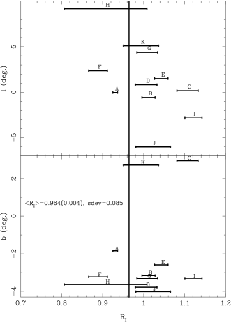
Figure 3: The ratio of total to selective extinction $R_{I}\equiv A_{I}/E(V-I)$ for each region as a function of Galactic coordinates. The values of $R_{I}$ correspond to the middle of the error bars, and the average $\langle R_{I}\rangle$ is shown with a vertical line.

Table 1: The ratio of total to selective extinction $R_{I}$ for each region.

Region	fields (BUL_SC)	$l(deg.)$	$b(deg.)$	$R_{I}$	$\sigma_{R_{I}}$	$sdev$
A	3 4 5 37 39	0.168	-1.844	0.930	0.006	0.031
B	22 23	-0.380	-3.155	1.012	0.016	0.033
C	43	0.370	2.950	1.107	0.026	0.027
D	1 38 45 46	1.030	-3.780	1.006	0.026	0.033
E	20 21 30 34	1.692	-2.593	1.043	0.016	0.028
F	2 31 32 33 35 36	2.560	-3.233	0.889	0.023	0.027
G	16 17 18 19 42	4.582	-3.322	1.009	0.025	0.032
H	8 9 10 11 12 13	9.360	-3.632	0.907	0.101	0.078
I	24 25 40 41	-2.632	-3.333	1.121	0.021	0.031
J	26 27 28 29	-5.805	-4.015	1.023	0.042	0.036
K	14 15	5.305	2.720	0.994	0.043	0.026
All	-	-	-	0.964	0.004	0.085
without A	-	-	-	1.026	0.008	0.075

Figure 4: The constant $I_{0,\rm RC}$ (cf. Eq. (3)) is shown for each region as a function of Galactic coordinates adopting a fixed value $R_{I}=0.964$. The values correspond to the middle of error bars. Note region (C) and (K) are fields with $b>0$.

Table 2: Extinction corrected $I$ magnitude of RCGs $I_{0,RC}$ measured with fixing $R_{I}=0.964$ for each region.

Region	$I_{0,RC}$	$\sigma_{I_{0,RC}}$	$sdev$	$I_{0,RC}^{*}$	$\sigma_{I_{0,RC}^{*}}$
A	14.625	0.003	0.034	14.652	0.024
B	14.700	0.005	0.036	14.728	0.024
C	14.808	0.009	0.042	14.835	0.025
D	14.576	0.004	0.034	14.603	0.024
E	14.551	0.003	0.031	14.578	0.024
F	14.491	0.003	0.028	14.518	0.024
G	14.453	0.004	0.033	14.480	0.024
H	14.371	0.016	0.077	14.398	0.028
I	14.808	0.005	0.041	14.836	0.024
J	14.772	0.006	0.036	14.799	0.024
K	14.529	0.005	0.026	14.557	0.024

Note: $I_{0,RC}^{*}$ represent the value after the zero-point correction.

4 Extinction Map

4.1 Relative Reddening

In this section we estimate the mean RCGs colours for each bin $\langle V-I\rangle_{\rm RC}$, and we transform them to the relative reddening, $E(V-I)_{\rm RC}=\langle V-I\rangle_{\rm RC}-\langle V-I\rangle_{0,\rm RC}$, assuming the intrinsic colour of RCGs $\langle V-I\rangle_{0,\rm RC}=1.0$. Then we estimate the relative extinctions in $V$-band ($A_{V,\rm RC}$) and $I$-band ($A_{I,\rm RC}$) by Eq. (2) and (1).

In the following analysis we adopt the reddening line with the slope $R_{I}=0.964$ and a constant $I_{0,RC}$ as given in table 2. Thanks to fixing $R_{I}$ and $I_{0,RC}$, we can get accurate $\langle V-I\rangle_{\rm RC}$ with a smaller number of RCGs, i.e. with high resolution in space (small bin) and in reddening (small group). Furthermore we introduce a new indicator $\langle V-I\rangle_{\rm all}$ which is the average colour of all stars in each bin, to represents the level of extinction in each bin to arrange bins into group. Because the number of all stars are much larger than RCGs, we to get higher spacial resolution.

We divide each field into a new set of small ”bins” with the size in the range $64\times 64$ to $157\times 157$ pixels, chosen so that each bin has $\sim 200$ stars. Next, we measure the average colour of all stars in each bin, $\langle V-I\rangle_{\rm all}$. We also measure the average colour of RCGs in each ”bin”, $\langle V-I\rangle_{\rm RC}$, following method [1] described in the previous section, with a radius of 0.5 mag, allowing the center of RCGs to lie only on the reddening line. The initial values of $\langle V-I\rangle_{\rm RC}$ for this method are estimated by using the parallelogram along this reddening line. This may be fairly uncertain statistically as there are only several RCGs per bin, but may suffer from less systematics than $\langle V-I\rangle_{\rm all}$. We compare the two sets of colours in Fig. 6 (upper sequence) for the field BUL_SC22. There is good correlation between $\langle V-I\rangle_{\rm RC}$ and $\langle V-I\rangle_{\rm all}$. Other fields have similar trends, but the slops are not always $1$. This good correlation imply that $\langle V-I\rangle_{\rm all}$ can be a good extinction indicator, as suggested by Popowski, Cook & Becker (2003).

We arrange bins in a given field in order of extinction by using $\langle V-I\rangle_{\rm all}$. Then we combine these bins into groups from low extinction to high extinction until each group is filled by $\sim 100$ RCGs. Note that groups in § 3 have $\sim 1,000$ RCGs.

In Fig. 5 we show an example of a CMD for two groups of bins in BUL_SC22, one with low extinction (filled circles) and one with high extinction (open circles). We calculate the average colour of RCGs $\langle V-I\rangle_{\rm RC,g}$ for each group of bins using the method described in previous paragraph. As described above, thanks to fixing $R_{I}$ and $I_{0,RC}$, we can get accurate $\langle V-I\rangle_{\rm RC,g}$ because the RCGs colour are very similar to the colours of red giants which are somewhat brighter or fainter than RCGs.

There is a very good correlation between these colours and $\langle V-I\rangle_{\rm RC}$ obtained for single bins, as shown in Fig. 6 (lower sequence). In this figure the typical width of $\langle V-I\rangle_{\rm RC}$ of bins in each group can be seen by the gaps of $\langle V-I\rangle_{\rm RC,g}$, about $<0.1$ mag depending on the number density of stars. We adopt $\langle V-I\rangle_{\rm RC,g}$ as the mean colour of RCGs for bins in this group, because these are based on the large statistics of RCGs.

Some bins were not included in any group for variety of reasons: (1) a bin has fewer than 20 stars, (2) a bin has a very bright blue star (mimics low extinction), (3) a bin has a very bright red star (mimics high extinction). (4) because of a very high extinction a large fraction of Bulge red giants is below the detection limit, so these bins can not be grouped properly with $\langle V-I\rangle_{\rm all}$ (in fields BUL_SC5 and BUL_SC37). If there were more than 5 RCGs in a given bin, then we adopted the average colour of these RCGs $\langle V-I\rangle_{\rm RC}$, which were estimated in the third paragraph of this section, as the mean colour of RCGs for this bin. Otherwise these bins are filled by the average value of the neighbours. $\langle V-I\rangle_{\rm RC}$ in each bin can not be used for the case (3), because stars reddened by bright red stars contaminate the RCG region in the CMD.

Problematic bins are flagged with ”-1” (1), ”-2” (2), ”-3” (3) and ”-4” (4). If $\langle V-I\rangle_{\rm RC}$ is adopted in a bin then this bin is flagged with the above value plus ”-10”.

We do not have confidence in measurements of $\langle V-I\rangle_{\rm RC}$ at $\langle V-I\rangle_{\rm RC}>4$, where the detection limit makes RCG centroid in the CMD systematically brighter and bluer. This implies that for $\langle V-I\rangle_{\rm RC}>4$ mag our maps give a lower limit to the extinction. We added ”-20” to the value of the flag of such bins. Only BUL_SC5 and BUL_SC37 suffer from this effect.

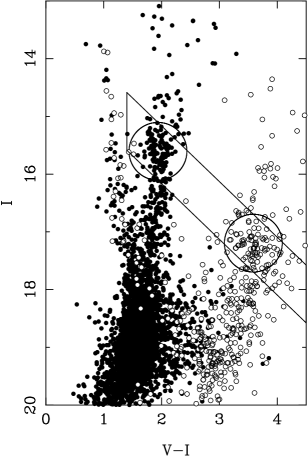
Figure 5: The CMDs of two groups in BUL_SC22. Filled and open circles represent stars in a group with low and high extinction, respectively. The elongated parallelogram represents the window used for the initial selection of RCGs. Two large circles indicate the RCG selection for the two groups.

Figure 6: The mean colour of RCGs $(V-I)_{\rm RC}$ in each bin as a function of the mean colour of all stars in the bin ($(V-I)_{\rm all}$, upper sequence) and the mean colour of RCGs in each group ($(V-I)_{\rm RC,g}$, lower sequence) in the field BUL_SC22. $(V-I)_{\rm RC,g}$ is shifted by +0.5 mag for clarity.

4.2 Zero point

We assume that the average colour of RCG stars, corrected for interstellar reddening, is the same in every field, and we ignore a possible weak dependence on metalicity (Paczyński & Stanek 1998). The zero-point of $\langle V-I\rangle_{\rm 0,RC}$ is calibrated following Alcock et al. (1998b). In Fig. 7, we show the offset of our relative extinction $A_{V,\rm RC}$ and $V$-band absolute extinction for 20 RRab in Alcock et al. (1998b), $A_{V,\rm RR}$. The average offset is $\langle A_{V,\rm RC}-A_{V,\rm RR}\rangle=0.055\pm 0.048$ with the standard deviation of $sdev=0.22$. The errors and $sdev$ are the same as in Alcock et al. (1998b) with Stanek (1996)’s map. This means that reddening corrected $\langle V-I\rangle$ colour and $\langle I\rangle$ magnitude of RCGs are given as $1+0.055/R_{VI}=1.028$ and the value of $I_{0,\rm RC}$ in table 2 plus $0.055R_{I}/R_{VI}=0.027$, respectively. The extinction corrected $I$-band magnitudes $I_{0,\rm RC}^{*}$ after zero-point correction are shown in table 2.

Our extinction and reddening maps are calibrated by this offset. We show the $A_{V}$ extinction maps in Fig. 8. The parameters: the bin-size, the number of groups, the total number of all stars, the average number of all stars in each bin, the total number of RCGs, the average number of RCGs in each group, the average values and errors in $E(V-I)$, $A_{V}$ and $A_{I}$ are given in Table 3. The values of $\langle\sigma\rangle$ are the statistical errors in relative maps, and they do not include zero-point errors $\sigma_{E(V-I),0}=0.024$, $\sigma_{A_{V},0}=0.048$ and $\sigma_{A_{I},0}=0.024$. To check our maps we present in Fig. 9 a comparison of $A_{V}$ in the relatively large overlap region of BUL_SC30 and BUL_SC31. One can see a good correlation between them in this figure, and $\chi^{2}/d.o.f.=1.15$ implies that our error estimate is reasonable.

Figure 7: Difference of relative extinction $A_{V,\rm RC}$ from RCGs (see §4.1) and $V$-band extinction from 20 RRab in Alcock et al. (1998b), $A_{V,\rm RR}$, i.e., the same figure as Fig. 3 of Alcock et al. (1998b).

Table 3: Basic parameters of maps, the bin-size, the number of groups, the total number of all stars, the mean number of all stars in each bin, the total number of RCGs, mean of RCGs in each group, the mean of values and errors in $E(V-I)$, $A_{V}$ and $A_{I}$.

BUL	binsize	$N_{\rm grp}$	$N_{\rm all}$		$N_{\rm RC}$		$E(V-I)$		$A_{V}$		$A_{I}$
_SC	(pixel)		total	mean	total	mean	mean	$\langle\sigma\rangle$	mean	$\langle\sigma\rangle$	mean	$\langle\sigma\rangle$
1	73.1	189	647014	203.1	18571	98.3	0.854	0.012	1.677	0.027	0.823	0.017
2	68.3	207	753366	198.4	20416	98.6	0.787	0.012	1.545	0.024	0.759	0.013
3	73.1	427	653389	205.3	42183	98.8	1.472	0.014	2.891	0.065	1.419	0.061
4	70.6	417	693066	197.7	41059	98.5	1.319	0.014	2.591	0.054	1.272	0.048
5	157.5	-	145562	209.2	21310	35.6	2.918	0.030	5.733	0.192	2.814	0.184
6	107.8	68	319093	221.0	6783	99.8	0.700	0.011	1.374	0.024	0.675	0.015
7	97.5	62	376688	210.3	6176	99.6	0.676	0.012	1.327	0.025	0.652	0.015
8	113.8	52	287653	214.7	4476	86.1	1.087	0.014	2.135	0.042	1.048	0.034
9	113.8	50	269318	197.2	4516	90.3	1.060	0.013	2.083	0.039	1.023	0.032
10	107.8	61	316050	219.4	5382	88.2	1.136	0.013	2.231	0.044	1.095	0.037
11	113.8	58	287074	220.4	4965	85.6	1.153	0.014	2.266	0.046	1.112	0.039
12	93.1	84	400853	215.7	7154	85.2	1.165	0.015	2.289	0.048	1.123	0.040
13	89.0	83	455162	212.6	7088	85.4	1.047	0.015	2.056	0.042	1.009	0.034
14	93.1	158	409086	201.4	15727	99.5	1.269	0.012	2.494	0.048	1.224	0.044
15	102.4	134	322254	221.3	13232	98.8	1.408	0.012	2.766	0.059	1.358	0.055
16	89.0	127	444114	232.1	11926	93.9	1.094	0.013	2.150	0.038	1.055	0.031
17	85.3	131	494911	213.3	12606	96.2	0.988	0.012	1.940	0.031	0.952	0.022
18	73.1	189	649856	196.7	18267	96.7	0.904	0.012	1.776	0.028	0.872	0.019
19	75.9	173	625566	203.6	16562	95.7	1.022	0.012	2.008	0.034	0.986	0.026
20	68.3	313	732180	193.8	30732	98.2	0.986	0.013	1.936	0.032	0.951	0.023
21	66.1	287	793369	197.6	27964	97.4	0.930	0.013	1.827	0.030	0.897	0.020
22	75.9	273	596019	194.3	26357	96.5	1.392	0.013	2.734	0.060	1.342	0.055
23	78.8	230	583168	204.6	22400	97.4	1.377	0.013	2.704	0.058	1.327	0.053
24	81.9	228	509439	196.1	22737	99.7	1.282	0.011	2.519	0.049	1.237	0.045
25	81.9	210	519559	198.7	20908	99.6	1.191	0.011	2.339	0.042	1.148	0.037
26	75.9	175	617829	201.2	16864	96.4	0.945	0.011	1.857	0.029	0.912	0.021
27	75.9	156	594953	193.9	15333	98.3	0.860	0.011	1.690	0.025	0.830	0.016
28	102.4	80	339107	201.0	7871	98.4	0.834	0.012	1.638	0.025	0.804	0.015
29	93.1	76	398252	194.7	7430	97.8	0.779	0.011	1.530	0.024	0.751	0.015
30	73.1	258	671739	211.3	25476	98.7	0.971	0.012	1.908	0.030	0.937	0.022
31	70.6	245	716500	204.2	24183	98.7	0.921	0.012	1.810	0.028	0.888	0.018
32	70.6	217	684274	200.0	21387	98.6	0.822	0.012	1.614	0.025	0.792	0.014
33	73.1	184	669836	202.6	17962	97.6	0.865	0.012	1.699	0.026	0.834	0.016
34	64.0	331	849632	198.4	31842	96.2	1.146	0.013	2.252	0.042	1.106	0.035
35	70.6	221	696335	196.7	21495	97.3	0.936	0.012	1.838	0.029	0.902	0.019
36	68.3	205	764524	201.5	19973	97.4	0.825	0.012	1.621	0.026	0.796	0.015
37	102.4	-	463048	274.3	37114	23.4	1.921	0.029	3.773	0.114	1.852	0.102
38	73.1	213	634009	199.2	21036	98.8	0.927	0.012	1.821	0.029	0.894	0.019
39	70.6	383	684042	193.9	37753	98.6	1.337	0.013	2.625	0.055	1.289	0.050
40	93.1	230	419439	206.9	22680	98.6	1.496	0.012	2.940	0.066	1.443	0.063
41	85.3	229	495001	205.2	22661	99.0	1.351	0.012	2.653	0.055	1.303	0.051
42	81.9	160	521529	198.2	14804	92.5	1.164	0.013	2.286	0.043	1.122	0.036
43	120.5	247	257326	216.0	25921	104.9	1.870	0.012	3.674	0.097	1.803	0.094
44	-	-	53346	-	1257	-	-	-	-	-	-	-
45	78.8	175	562718	205.4	17247	98.5	0.836	0.012	1.642	0.028	0.806	0.018
46	85.3	159	495299	213.1	15643	98.4	0.871	0.012	1.711	0.029	0.840	0.019
47	128.0	58	209811	194.4	4986	86.0	1.321	0.015	2.595	0.056	1.274	0.049
48	128.0	57	217083	201.0	5229	91.7	1.194	0.014	2.346	0.046	1.152	0.039
49	136.5	43	193318	203.5	4086	95.0	1.063	0.014	2.089	0.038	1.025	0.030

Note: $\langle\sigma\rangle$ do not include zero-point errors $\sigma_{E(V-I),0}=0.024$, $\sigma_{A_{V},0}=0.048$ and $\sigma_{A_{I},0}=0.024$.

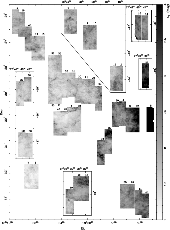
Figure 8: $A_{V}$ Extinction map. Distant fields are in small boxes. Gray scale is shown at the right corner.

Figure 9: Comparison of $A_{V}$ of overlap region in BUL_SC30 and in BUL_SC31.

We show the histogram of $E(V-I)$ for all our maps in Fig. 10. The vertical line indicates the threshold value $E(V-I)_{\rm th}=3.0$, which corresponds to $\langle V-I\rangle_{\rm RC}=4$ mag. We have confidence in our maps below this threshold. However, small, very heavily obscured regions are above this reddening threshold, pushing some RCGs below the OGLE-II detection limit, and distorting the RCGs. This implies that for $\langle V-I\rangle_{\rm RC}>4$ mag our maps give a lower limit to the extinction. Histograms of $A_{V}$ and $A_{I}$ can be obtained by multiplying $E(V-I)$ by $R_{VI}$ and $R_{I}$ respectively. The thresholds are: $A_{V,\rm th}=5.8$ and $A_{I,\rm th}=2.9$.

Figure 10: A histogram of $E(V-I)$ for all our maps. Vertical line indicates the threshold value $E(V-I)_{\rm th}=3.0$ mag.

The reddening corrected value of $(V-I)_{\rm 0,RC}$ may vary from one field to another due to weak dependence on metalicity. The RR Lyrae variables are good distance indicators (e.g., Nemec, Nemec & Lutz 1994) whose period-luminosity relations are well established (Jones, Carney, Storm & Latham 1992). The RR Lyrae lie in the instability strip, the range of their colour is small and it weakly depends on period, amplitude and/or metallicity (Bono, & Stellingwerf 1994; Alcock et al. 1998a). To check the relative zero-points of our reddening maps for each field we make use of the $V-I$ colour of RR Lyrae Type ab (RRab), assuming that period - $(V-I)_{0}$ colour relation of RRab is the same for all OLGE-II fields

We selected RRab in OGLE-II Galactic Bulge variable star catalogue (Woźniak et al. 2001) by using the method of Alard (1996). We measured periods $P$ using PDM algorithm (Stellingwerf 1978) and Fourier coefficients by fitting Fourier series with five harmonics. In Fig 11 we show the the amplitude ratio $R_{21}\equiv A_{2}/A_{1}$ versus phase differences $\phi_{21}\equiv\phi_{2}-2\phi_{1}$ for variables with $P<0.9$ days, except $0.4985<P<0.5001$ days, which are affected by aliasing. We selected 1,961 RRab stars as a clear clump within the ellipse in this figure. Of these 1,819 stars have $\langle V\rangle$ and $\langle I\rangle$ photometry provided by Udalski (2003). We visually inspected all light curves and several stars with non RR Lyrae shape light curves were rejected. In Fig 12 we present colour - magnitude diagram for RRab stars so selected. The differential reddening is apparent. A similar reddening slope is found in §3.

In the following analysis we rejected 39 stars with $I<1.1(V-I)+13.1$ because they are either nearby disk stars or they are blended with other bright stars. We did not reject several background RRab below the sequence as they made no difference to our analysis, for which we used 1,780 RRab stars.

Figure 11: $R_{21}$ v.s. $\phi_{21}$ for periodic variables in the OGLE catalogue. RRab variables are selected within the ellipse. There is a clump of RRc variables below the ellipse, but we do not use them in this work.

Figure 12: The CMD for RRab variables. Solid line with a slope of $I/(V-I)=1.0$ is shown as a reference. RRab variables above the dashed line: $I=1.1(V-I)+13.1$ are rejected in our analysis because they are foreground disk stars or variables blended with other bright stars.

We assume that reddening corrected colour $(V-I)_{\rm 0,RR}$ is the same in every field, with a possible weak dependence on period $P$, or amplitude $A$, or both. We estimate the zero-points $C_{i}$ for each field $i$ by fitting extinction corrected colour of RRab with a linear dependence on $\log P$, $A$, and on both of them. We obtained the following relations:

$$(V-I)_{\rm 0,RR} = 0.309(\pm 0.049){\rm log}P+C_{i},sdev=0.158,$$ (6)

$$(V-I)_{\rm 0,RR} = -0.096(\pm 0.016)A+C_{i},sdev=0.157,$$ (7)

$$(V-I)_{\rm 0,RR} = 0.211(\pm 0.056){\rm log}P-0.063(\pm 0.018)A$$ (8)

$$+ C_{i},sdev=0.156.$$

All three relations provided almost the same values of $C_{i}$. Fitting with both $P$ and $A$ seems to be an over-parameterization.

In Fig. 13, we show extinction corrected colours of RCGs $(V-I)_{\rm 0,RC}$ (open circle) and RRab $(V-I)_{\rm 0,RR}$ (filled circle and errors) as a function of the galactic $l$ and $b$, where $(V-I)_{\rm 0,RC}$ are measured by the method [3] in § 3 and $(V-I)_{\rm 0,RR}$ are the value given by Eq. (6) at log$P=-0.3$.

$(V-I)_{\rm 0,RC}$ is constant as assumed. The mean of $(V-I)_{\rm 0,RC}=1.0283\pm 0.024$, where we used $\sigma_{E(V-I),0}=0.024$ as the error in $(V-I)_{\rm 0,RC}$, is consistent with the colour of nearby RCGs $(V-I)_{\rm 0,RC,near}=1.01\pm 0.08$ mag (Paczyński & Stanek 1998), contrary to $(V-I)_{\rm 0,RC,bulge}=1.11\pm 0.12$ by Paczyński et al. (1999) with Stanek (1996)’s map.

$(V-I)_{\rm 0,RR}$ seems to be systematically redder by about $\sim 0.1$ mag at large $|l|$. Such trend can not be seen in $b$. We plot $(V-I)_{\rm 0,RR}$ as a function $|l|$ in Fig. 14 and we fit it with a straight line for $|l|<6$ (filled circle and solid line) and for $|l|>6$ (open circle and dashed line). One can see the RRab colour is constant at $|l|<6$ and have a significant ($3\sigma$) dependence on $|l|$ at $|l|>6$. The mean $(V-I)_{\rm 0,RR}$ is $0.4670\pm 0.0047$ with $sdev=0.0286$ for $|l|<6$ and $0.5386\pm 0.0126$ with $sdev=0.0773$ for $|l|>6$. The significance of the redder colour in $|l|>6$ is estimated to be $5.3\sigma$ level.

This implies that $(V-I)_{\rm 0,RC}$, $(V-I)_{\rm 0,RR}$ or both of them, may vary with $l$. If we assume that $(V-I)_{\rm 0,RR}$ is constant, then the intrinsic colour of RCGs would be bluer, i.e., the zero-points of our reddening maps would be smaller by $\sim 0.1$ mag at $|l|=10$, compared to $|l|\leq 6$. This could be explained if the outer RCGs have lower metalicity and are somewhat bluer than near the Galactic Center. The colour of RRab $(V-I)_{\rm 0,RR}=0.4\sim 0.5$ for $|l|\leq 6$ is consistent with the colour of local RRab, while the two sets of colours were claimed to be different by Stanek (1996)’s map by Stutz, Popowski & Gould 1999.

The scatter of $(V-I)_{\rm 0,RR}$ values is large because public domain $V$-band OGLE photometry is the average of randomly distributed small number of $V$-band measurements, while the $V$ amplitude is large. Furthermore the scatter is larger for $|l|>6$ because the number of RRab is small in these fields. Therefore, we do not correct for the offsets apparent in Fig. 13. It will be possible to improve the accuracy of $(V-I)_{\rm 0,RR}$ when individual $V$-band measurements become available.

Figure 13: Extinction corrected colours of RCGs $(V-I)_{\rm 0,RC}$ (open circle) and RRab $(V-I)_{\rm 0,RR}$ (filled circle and errors) as a function of the galactic $l$ and $b$. $(V-I)_{\rm 0,RR}$ are the value given by Eq. (6) at log$P=-0.3$. Solid line represent a mean of $(V-I)_{\rm 0,RC}=1.0283\pm 0.024,sdev=0.0034$, where the error in $(V-I)_{\rm 0,RC}$ is dominated by $\sigma_{E(V-I),0}=0.024$.

Figure 14: Extinction corrected colours of RRab $(V-I)_{\rm 0,RR}$ as a function of the absolute galactic $|l|$. $(V-I)_{\rm 0,RR}$ are the value given by Eq. (6) at log$P=-0.3$. Filled and open circles represent plots in $|l|<6$ and in $|l|>6$, and solid and dashed lines indicate the best fits for them, respectively. One can see the RRab colour is constant at $|l|<6$ and significantly red at $|l|>6$.

5 Discussion and Conclusion

We confirmed the anomalous reddening, i.e. a small value of the ratio of total to selective extinction $R_{VI}=1.9\sim 2.1$ depending on the line of sight, as measured by Udalski (2003). This implies that the distribution of dust grains may be tipped to smaller sizes in these regions, compared to average in the Galaxy. A detailed analysis of these results is beyond the scope of the present study.

By adopting the mean value of $R_{VI}=1.964$, we have constructed reddening $E(V-I)$ and extinctions, $A_{V}$ and $A_{I}$ maps in 48 OGLE-II GB fields, covering a range of $-11^{\circ}<l<11^{\circ}$, with the total area close to 11 square degrees. The reddening $E(V-I)$ and extinctions, $A_{V}$ and $A_{I}$ are measured in the range $0.42<E(V-I)<3.5$ mag, $0.83<A_{V}<6.9$ mag and $0.41<A_{I}<3.4$. Note: above the threshold values $E(V-I)_{\rm th}=3.0$, $A_{V,\rm th}=5.8$ and $A_{I,\rm th}=2.9$, which correspond to $\langle V-I\rangle_{\rm RC}=4$ mag, our maps give the lower limit to reddening and extinction. Spatial resolutions of maps are $26.7^{\prime\prime}\sim 106.8^{\prime\prime}$ depending on the stellar density of each field.

The absolute zero-point is calibrated using 20 RRab variables in Baade’s Window, following Alcock et al. (1998b). Relative zero-points of our maps are verified with 1,780 RRab variables found in our fields. We found that these zero-points may be lower by $\sim 0.1$ mag at larger Galactic longitudes $|l|>6$. Note that our extinction map is OK in terms of the relative extinction within each field. The relative zero points are also OK between fields for $|l|<6$. We did not make any correction for this effect in the paper.

We used the mean value of $R_{VI}=1.964$, but different fields have a range of values, with a standard deviation $sdev\sim 0.085$ (see Fig.3). We estimated the errors of our maps by taking this range into account. The errors approach $0.17$ mag at the highest extinction ($A_{V}=6$).

As noted by Udalski et al. (2002) and Udalski (2003), the $I$-band filter used by OGLE-II has the red wing somewhat wider than standard. This may lead to systematic deviations from the standard values for very red stars, giving brighter $I$-band magnitudes (redder $V-I$ colour) for the OGLE-II filter for very red stars ($V-I>2$), while the error is negligible in the range where the OGLE-II data were calibrated by standards, i.e. for ($V-I<2$). This effect may reach $\sim 0.2$ mag for the very red RCGs ($V-I>4$ mag). This effect makes the slope of reddening line in the CMD somewhat shallower, as shown by Udalski (2003). This effect is not sufficient to explain the anomalous extinction towards the GC. Udalski (2003) analyzed the differences between OGLE-II and standard $I$-band filters using Kurucz (1992)’s model atmosphere of a typical RCGs, reddened with the standard interstellar extinction of Cardelli, Clayton& Mathis (1989) and Fitzpatrick (1999). He found possible errors to be at the level $\pm 0.1$ in $R_{VI}$, depending on the model of extinction and the colour range of RCGs in each field. This leads to $\sim 0.2$ mag differences in $E(V-I)$, $A_{V}$ and $A_{I}$ for the very red RCGs, with $V-I>4$ mag, corresponding to $E(V-I)\sim 3$, $A_{V}\sim 5.9$ and $A_{I}=2.9$ mag in our extinction maps. These differences are the upper limits because the atmospheric absorption in the range 900-990 nm makes the OGLE-II $I$-band filter closer to the standard one (Udalski et al. 2002). To make a more accurate estimate of the required correction it is necessary to have very red standard stars, with $(V-I)>2$.

The extinction corrected $I$-band magnitude of RCGs, $I_{0,RC}^{*}=14.6$ in Baade’s window is fainter than expected. Adopting distance modulus to the GC of $14.52\pm 0.1$ mag (Eisenhauer et al. 2003), and assuming that the population of RCG stars in the Galactic bulge is the same as local, i.e. that the absolute magnitude is $M_{I_{0,RC}}=-0.26\pm 0.03$ (Alves et al. 2002) and the average colour is $(V-I)_{0}=1.01\pm 0.08$ (Paczyński & Stanek 1998), then the expected magnitude of RCG in Baade’s Window should be $I_{0,RC}=14.3$. In Fig. 15 we show CMD and RCG centroids of BUL_SC1 (at Baade’s window) before (left panel) and after (right panel) the extinction and reddening correction, with the expected RCG centroid. Note, that the difference between the average distance modulus in Baade’s Window and the Galactic center is only 0.02 mag, i.e. it is of no consequence (Paczyński & Stanek 1998).

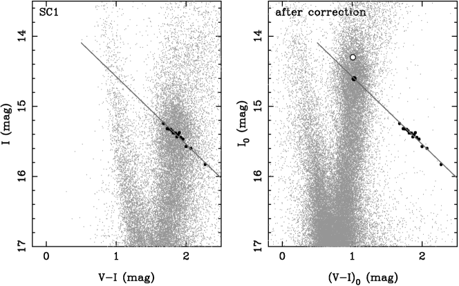
Figure 15: Colour Magnitude Diagram of BUL_SC1 before (left panel) and after (right panel) the extinction and reddening correction. Small and large filled circles indicate the same plots as Fig. 2 and RCGs centroid after the extinction and reddening correction. Open circle represents the RCGs centroid expected from the assumption that the population of RCGs in GB is the same as local. The solid line indicate the reddening line given by Eq. 3 with the mean slope $R_{I}=0.964$ and a constant $I_{0,RC}=14.6$ for this field.

We do not know what is the solution of this problem. It may be that the population effects are large $M_{I_{0,RC}}=-0.4\sim-0.03$, as claimed by Salaris et al. (2003) and Percival & Salaris (2003), it may be that the distance to the GC is larger, or it is possible that the reddening is more complicated. We assumed that the extinction to reddening ratio is constant all the way to zero extinction. OGLE photometry is well calibrated with standards for $(V-I)<2$. The slope of the reddening line in Baade’s Window (Region D) is well measured for RCG in the colour range $1.6<(V-I)<2.2$, but we have no direct information about the reddening line for $1.0<(V-I)<1.6$, i.e. for the reddening range $0<E_{V-I}<0.6$. If we make an ad hoc assumption that the RCG population in Baade’s Window is the same as local, and the distance is 8 kpc, then we may obtain $I_{0,RC}^{*}=14.3$ and $(V-I)_{0,RC}=1.0$ adopting $R_{VI}\sim 2.8$ (i.e. $R_{I}\sim 1.8$)for the unobserved range $0<E_{V-I}<0.6$. We do not know if this is plausible or not.

The situation will improve somewhat once detailed $V$-band OGLE photometry becomes available for RR Lyrae stars, and this will make it possible to obtain an independent estimate of the reddening in Baade’s Window. Preliminary analysis of the average photometry of RR Lyrae stars seems to indicate that the puzzling brightness of red clump giants may be due to population effects, i.e. their average absolute magnitude in the Bulge is somewhat different than it is near the Sun. A much improved analysis will be done when OGLE-II $V$-band measurements become available in the next several months. At this time it should be OK to use our maps of differential reddening, but we consider our calibration of zero point to be uncertain. This implies that at this time our reddening maps are not adequate for a quantitative study of Galactic bar structure.

In this work we leave our extinction maps in the OGLE-II $I$-band because the reddening map is urgently needed for various applications, and is already used in some works (Sumi et al. 2003b; Wray, Eyer & Paczyński 2003). A reader must take care of possible small error mentioned above while using our maps for standard $I$-band photometry.

The extinction map is available in electronic format via anonymous ftp from the server ftp://ftp.astrouw.edu.pl/ogle/ogle2/extinction/ and ftp://bulge.princeton.edu/ogle/ogle2/extinction/.

These extinction maps of OGLE-II GB fields facilitate the study of the Galactic structure with OGLE proper motion catalogue (Sumi et al. 2003b) and microlensing optical depth, and a study of variable stars, but the reader should be aware of the zero point of the extinction may not be accurate. We intend to improve the quality of the zero points in all fields as soon as individual OGLE $V$-band measurements of the RR Lyrae stars become available.

References

- Afonso et al. (2003) Afonso, C. et al. 2003, A&A in press, preprint (astro-ph/0303100)
- Alard (1996) Alard, C. 1996, ApJ, 458, L17
- Alcock et al. (1997) Alcock, C. et al. 1997, ApJ, 486, 697
- Alcock et al. (1998a) Alcock, C. et al. 1998a, ApJ, 492, 190
- Alcock et al. (1998b) Alcock, C. et al. 1998b, ApJ, 494, 396
- Alcock et al. (2000) Alcock, C. et al. 2000a, ApJ, 541, 734
- Alves et al. (2002) Alves, D. R. et al. 2003, ApJ, 573, L51
- Bond et al. (2001) Bond, I. A. et al. 2001, MNRAS, 327, 868
- Cardelli, Clayton& Mathis (1989) Cardelli, J. A., Clayton, G. C. & Mathis, J. S., 1989, ApJ, 345, 245
- Derue (1999) Derue, F. et al. 1999, A&A, 351, 87
- Dutra et al. (2003) Dutra, C. M., Santiago, B. X., Bica, E. L. D. and Barbuy, B. 2003, MNRAS, 338, 253
- Eisenhauer et al. (2003) Eisenhauer, F. et al. 2003, preprint (astroph/0306220)
- Fitzpatrick (1999) Fitzpatrick, E. L. 1999, PASP, 111, 63
- Gould (1996) Gould, A. 1996, PASP, 108, 465
- Gould, Popowski & Terndrup (1998) Gould, A., Popowski, P. & Terndrup, D. M. 1998, ApJ, 492, 778
- Jones, Carney, Storm & Latham (1992) Jones, R. V., Carney, B. W., Storm, J. & Latham, D. 1992, ApJ, 386, 646
- Bono, & Stellingwerf (1994) Bono, G. & Stellingwerf, R. F. 1994, ApJ, 93, S233
- Kiraga, Paczyński & Stanek (1997) Kiraga, M., Paczyński, B. & Stanek, K. Z., 1997, ApJ, 485, 611
- Kurucz (1992) Kurucz, R. L. 1992, IAU Symp. 149, The Stellar Populations of Galaxies, ed.B.Barbuy & A. Renzini (New York:Springer), 225
- Ng et al. (1996) Ng, Y. K., et al. 1996, A&A, 310, 771
- Nemec, Nemec & Lutz (1994) Nemec, J. M., Nemec, A. F. L. & Lutz, T. E. 1994, AJ, 108, 222
- Paczyński (1996) Paczyński, B. 1996, ARA&A, 34, 419
- Paczyński & Stanek (1998) Paczyński, B. & Stanek, K. Z. 1998, ApJ, 494, L219
- Paczyński et al. (1999) Paczyński, B. et al., 1999, Acta. Astron.,49, 319
- Percival & Salaris (2003) Percival, S. M. & Salaris, M. 2003, MNRAS, 343, 539
- Popowski (2000) Popowski, P. 2000, ApJ, 528, L9
- Popowski et al (2003) Popowski, P. et al. 2003, Invited Review, to appear in ”Gravitational Lensing: A Unique Tool For Cosmology”, Aussois 2003, eds. D. Valls-Gabaud & J.-P. Kneib (astro-ph/0304464)
- Popowski, Cook & Becker (2003) Popowski, P., Cook, K., Becker, B. 2003, AJ, in press
- Salaris et al. (2003) Salaris, M., Percival, S., Brocato, E., Raimondo, G., Walker, A. R., 2003 ApJ, 588, 801