Towards Constraints on Dark Energy from Absorption Spectra of Close Quasar Pairs

Abstract

A comparison between the line of sight power spectrum (the auto spectrum) of absorption in the Lyman-alpha forest and the cross power spectrum (the cross spectrum) between the absorption in neighboring lines of sight offers an evolution-free means to constrain the cosmological constant, or dark energy. Using cosmological simulations, we consider a maximum likelihood method to obtain constraints from this comparison. In our method, measurements of the auto and cross spectra from observations are compared with those from a multi-parameter grid of simulated models of the intergalactic medium (IGM). We then marginalize over nuisance parameters to obtain constraints on the cosmological constant. Redshift space distortions due to peculiar velocities and thermal broadening, a potential difficulty in applying this test, are explicitly modeled in our simulations. To illustrate our method, we measure the cross spectrum from a new sample of five close quasar pairs, with separations of 0.5 to 3 arcmin. Using published measurements of the auto spectrum and our measurements of the cross spectrum, we attempt to obtain a constraint on $\Omega_{\Lambda}$, but find only weak constraints. An Einstein-de-Sitter cosmology is, however, disfavored by the data at a $\sim 2\sigma$ confidence level. We consider the power of future observations, paying particular attention to the effects of spectral resolution and shot-noise. We find that $\sim 50$ moderate resolution, FWHM $\sim 150$ km/s, fully-overlapping, close separation pairs (with $\Delta\theta\sim 30^{\prime\prime}-120^{\prime\prime}$) should allow a ($2\sigma$) constraint on $\Omega_{\Lambda}$ at the level of $15\%$, if other modeling parameters are well determined through other means. We find that there is a sizeable gain from observing very close, $\Delta\theta\sim 30^{\prime\prime}$, separation pairs provided they are observed with high spectral resolution. A sample of $\sim 10$ such pairs would yield similar constraints to the $50$ moderate resolution pairs mentioned above.

1 Introduction

In the last several years, much work has been done on the measurement of the flux/transmission auto power spectrum from the Lyman-alpha forest, and the derivation of cosmological constraints from it (e.g. Croft et al. 1998,1999,2002, Hui 1999, McDonald et al. 2000, Zaldarriaga, Hui & Tegmark 2001, Zaldarriaga, Scoccimarro & Hui, 2003, Gnedin & Hamilton 2002). Motivated by these developments, it is natural to extend observations and simulations to compare the cross-correlation, or in Fourier space the cross spectrum, between the absorption in neighboring lines of sight. Measuring the flux cross spectrum is a more ambitious project observationally than measuring the auto spectrum because extracting a good signal requires Ly$\alpha$ forest spectra of many close quasar pairs, which are rare. However, good observations of the Ly$\alpha$ forest in a handful of close quasar pairs have already existed for several years (Bechtold et al. 1994, Crotts & Fang 1998, Petitjean et al. 1998), and yielded information on the size and shape of Ly$\alpha$ absorbers. Theoretically, simulating the cross-correlation is challenging since it depends more sensitively on redshift distortions than the auto spectrum, the detailed modeling of which requires large volume, high resolution simulations. Although difficult to obtain, the information contained in the cross-correlation signal is rich. In particular, using the auto spectrum of the absorption in the Ly$\alpha$ forest and the cross spectrum one can constrain the cosmological constant or dark energy through a version of the Alcock-Paczyński (AP) test (Alcock & Paczyński 1979, McDonald & Miralda-Escudé 1999, Hui, Stebbins & Burles 1999, McDonald 2003, Lin & Norman 2002, Rollinde et al. 2003). In spite of this, little work has been done in comparing pair spectra with simulations using the modern picture of the Ly$\alpha$ forest and focusing on continuous-field statistics. (See however Rollinde et al. 2003.)

As a step in this direction, this paper aims to measure the cross spectrum from data and from simulations. Our present data set, consisting of five pairs with $z\gtrsim 2.2$, includes two new pairs and a triplet from Crotts & Fang (1998). From our measurements of the cross spectrum, which have large error bars owing to the small number of pairs in our current sample, and using the precise measurements of the auto spectrum from Croft et al. (2002), we attempt to obtain a constraint on the cosmological constant.

It is appropriate to ask: why carry out this exercise if we already know the value of the cosmological constant to fair accuracy from supernova measurements (Riess et al. 1998, Perlmutter et al. 1999), especially when used in conjunction with the microwave background anisotropies (Spergel et al. 2003)? The answer lies partly in the elegance of the Alcock-Paczyński test, in that it does not require a standard candle, and is therefore free of assumptions about evolution. The application to the Ly$\alpha$ forest of course suffers from systematics of its own. It is the cross-checks provided by different methods that give us confidence in our current picture of the universe. The present paper should be viewed as a warm-up exercise – as quasar pair samples increase in size, the method described here might prove to give competitive constraints on the cosmological constant/dark energy, and as will be discussed below, the resulting constraints will be nicely complementary to those from other methods.

The paper is organized as follows. In §2 we briefly review the AP test, its application using the Ly$\alpha$ forest and its sensitivity to cosmological parameters, especially dark energy. In §3 we describe the statistics that we use in our implementation of the AP test and describe how we measure them from simulations. In §4 we describe and quantify the effect of redshift distortions on the three-dimensional flux power spectrum by measurements from simulations. In §5 we present measurements of the cross spectrum from a small sample of quasar pairs and attempt to place a constraint on the cosmological constant from the measurements. The constraint comes from comparing simulated auto and cross spectra from a grid of models with the observed auto and cross spectra. The grid of models examined here is rather small, but our constraints are correspondingly weak. In §6 we consider the possibilities for constraining dark energy with future observations and consider the dependence on spectral resolution and shot noise. This section should be helpful in planning future observations. In §7 we conclude. In Appendix A we include some details concerning the simulations we run and show resolution and boxsize tests.

2 The AP Test

In this section we briefly review the AP test and its application in the Ly$\alpha$ forest. Alcock & Paczyński (1979) considered an astrophysical object, with redshift extent $\Delta z$ and angular extent $\Delta\theta$, and pointed out that the object’s inferred shape depends on cosmology. To be specific, the dependence on cosmology is as follows. The length of the hypothetical object along the line of sight in velocity units is $u_{\parallel}={{c\Delta z}\over{1+z}}$, and its perpendicular extent in velocity units is $u_{\perp}={H(z)\over 1+z}D_{A}(z)\Delta\theta$. Here $z$ is the mean redshift of the object, and $H(z)$ and $D_{A}(z)$ are respectively the Hubble parameter and the co-moving angular diameter distance at the mean redshift. The radiation-free Hubble parameter is $H(z)=H_{0}\left[\Omega_{m}(1+z)^{3}+\Omega_{k}(1+z)^{2}+\Omega_{\Lambda}\right]^{1\over 2}$, where $H_{0}$ is the present day Hubble parameter, and $\Omega_{m},\Omega_{k},\Omega_{\Lambda}$ are the present day matter, curvature and cosmological constant contributions to the energy density. The curvature density is related to the matter and cosmological constant densities by $\Omega_{k}=|1-\Omega_{m}-\Omega_{\Lambda}|$. The co-moving angular diameter distance, (as opposed to the proper angular diameter distance), is $D_{A}(z)={c\over H_{0}}{1\over\sqrt{\Omega_{k}}}S_{k}\left[\sqrt{\Omega_{k}}\int_{0}^{z}{dz^{\prime}\over H(z^{\prime})/H_{0}}\right]$. The function $S_{k}(x)$ that appears in the angular diameter distance is $S_{k}(x)=\sin(x)$ for a closed universe, $S_{k}(x)=\sinh(x)$ for an open universe and $S_{k}(x)=x$ for a flat universe, in which case $D_{A}(z)$ is just the co-moving distance out to redshift z.

The ratio, $u_{\parallel}\over u_{\perp}$, is a measure of the object’s shape, equal to one for spherical objects. The cosmological dependence of this ratio means that observers converting angles and redshifts to distances assuming different cosmologies will reach different conclusions about the object’s shape. One can assume any possible value of the cosmological parameters $\Omega_{m}$, $\Omega_{\Lambda}$; if the assumed parameters differ from the true cosmology, an object’s inferred shape will be distorted from its true shape. In particular we consider the distortion an observer assuming an Einstein-de-Sitter (EDS) cosmology measures in a universe with a cosmological constant (a Lambda cosmology), or any other postulated “true” cosmology. We define a squashing factor, $g_{\rm squash}(z)$, to quantify the distortion in the object’s shape (see e.g. Ballinger et al. 1997),

$$g_{\rm squash}(z)=\left({{u^{\prime}_{\perp}}\over{u^{\prime}_{\parallel}}}\right)\left({{u_{\parallel}}\over{u_{\perp}}}\right)={{H^{\prime}(z)D^{\prime}_{A}(z)}\over{H(z)D_{A}(z)}}$$ (1)

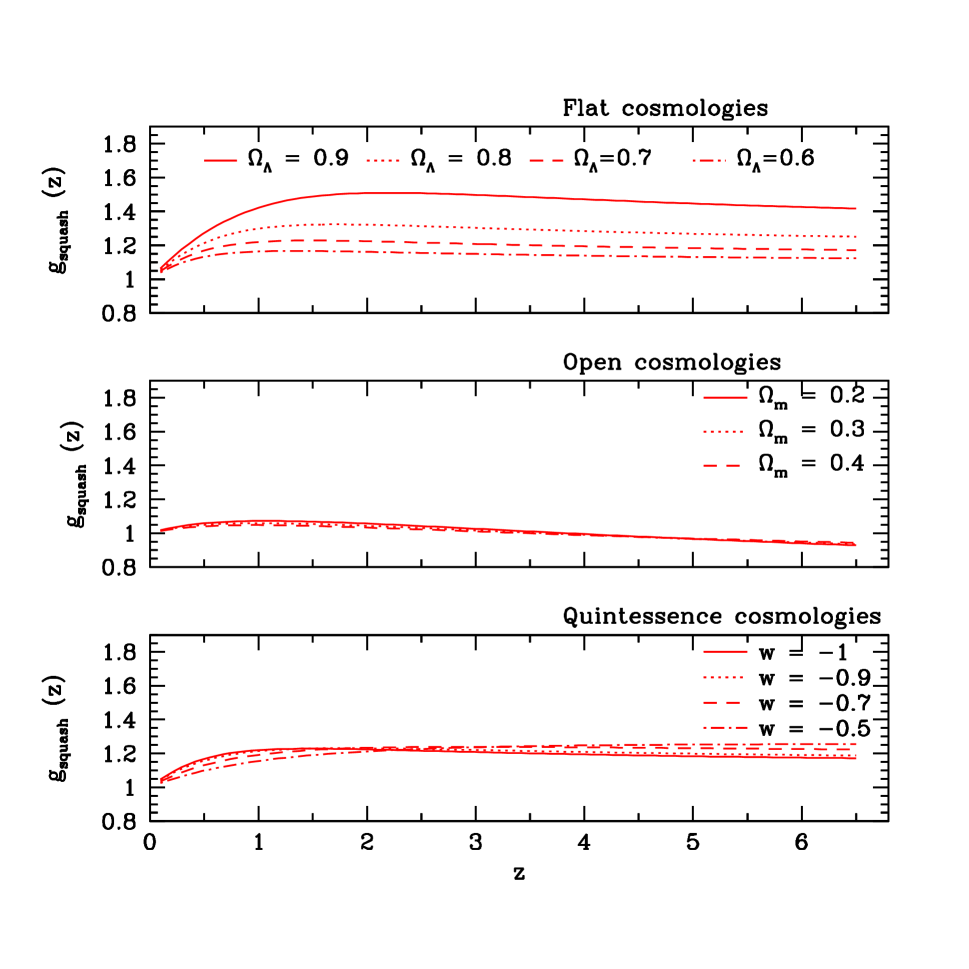
Figure 1: The top panel shows the squashing factor, $g_{\rm squash}(z)$, defined in §2, as a function of redshift for various flat, Lambda cosmologies. The middle panel shows the same factor for open universes. The bottom panel shows the squashing factor for flat quintessence models with $\Omega_{m}=0.3$. The equation of state of the quintessence field is assumed to be constant as a function of redshift. In each panel, the squashing factor is defined relative to the EDS case; it is the squashing an observer converting angles and redshifts to distances assuming an EDS cosmology would measure in a given “true” cosmology.

The primed variables represent coordinates in the EDS cosmology and the unprimed variables denote coordinates in the Lambda (or other postulated “true”) cosmology. This ratio is larger than one in the case of a Lambda cosmology; ${{H^{\prime}(z)D^{\prime}_{A}(z)}\over{H(z)D_{A}(z)}}>1$. The object appears squashed along the line of sight to the observer converting redshifts and angles to distances assuming an EDS cosmology; i.e., a spherical object with true dimensions $u_{\parallel}=u_{\perp}$, seems squashed by a factor $g_{\rm squash}$ so that $u^{\prime}_{\perp}>u^{\prime}_{\parallel}$. In figure (1) we plot the squashing factor, $g_{\rm squash}(z)$, as a function of redshift for several different cosmological models. In each case, the squashing factor shown is the squashing an EDS observer measures in a given “true” cosmology. In the top panel we show the squashing factor for several different values of $\Omega_{\Lambda}$, assuming a flat universe. In the middle panel we show the squashing factor assuming an open universe with no cosmological constant. The squashing factors in the open universe, zero cosmological constant models are close to unity, the squashing effect is always $\lesssim 10\%$ and typically only a $\sim 5\%$ effect in these models. As we can see in the top panel of the figure, the squashing effect is rather sensitive, however, to the presence of a cosmological constant. The squashing factor in the flat, Lambda universes shown here rises quickly with redshift, but plateaus around $z\sim 1$. After reaching this plateau, the squashing effect is only a $\sim 20\%$ effect for an $\Omega_{\Lambda}=0.7$ universe, but is a $\sim 50\%$ effect for an $\Omega_{\Lambda}=0.9$ flat universe. The plateau effect arises because the squashing is sensitive to the presence of a cosmological constant, which is small at high redshift. At redshifts beyond the plateau, the AP test should be particularly good at constraining the existence of a very large cosmological constant.

We also consider the sensitivity of the AP test to the equation of state of a dark energy, or quintessence, component to the energy density (Hui, Stebbins & Burles 1999). The equation of state of the quintessence component is parameterized by $p=w\rho_{Q}$, where $p$ is the (negative) pressure, and $\rho_{Q}$ is the component’s energy density. Here we consider the equation of state to be constant as a function of redshift, in which case $\rho_{Q}=\Omega_{Q}(1+z)^{3(1+w)}$. In the bottom panel of figure (1) we plot the squashing factor as a function of redshift for a few different quintessence cosmologies. At redshifts near $z=3$, where one can apply the AP test to the Ly$\alpha$ forest, the squashing factor is extremely similar for all of the quintessence cosmologies considered. This is in accord with McDonald (2003), (see also Kujat et al. 2002), who notes that this insensitivity to $w$ makes the Ly$\alpha$ forest a particularly good probe of $\Omega_{m}$ since constraints obtained on $\Omega_{m}$ are then insensitive to prior assumptions regarding $w$. The squashing factor at this redshift is more sensitive to the equation of state of dark energy, $w$, if $w(z\sim 3)\gtrsim-0.4$, however (McDonald 2003). For instance, as the equation of state of the dark energy approaches the limiting case of $w=-1/3$ the effect approaches that of an open cosmology, which has a significantly different squashing factor than a universe with a cosmological constant ($w=-1$). At lower and higher redshifts, the squashing factor is more sensitive to the equation of state, $w$. At low redshift the difference between squashing factors for the different quintessence cosmologies peaks near $z\sim 0.5$. The difference between squashing factors in a $w=-0.5$ cosmology and in a $w=-1$ cosmology is still only $\sim 6\%$ near this redshift, but the clustering of low/intermediate redshift objects is certainly a better probe of $w$ than the Ly$\alpha$ forest at $z\sim 3$. For instance, Matsubara & Szalay (2002) suggest applying the AP test using the clustering of luminous red galaxies, as a good low/intermediate redshift sample, to constrain $w$. At any rate, we now have an idea of the size of the geometric distortion in different cosmologies, and proceed to discuss some complications in applying the AP test with real ’astrophysical objects’.

To apply this test in the pure form mentioned above, one needs a spherical object or an object of other known shape, expanding with the Hubble flow. The three-dimensional power spectrum of galaxy or quasar clustering, $P(k)$, for instance, could provide such an object since it should be spherical by the cosmological principle if measured in real space (see e.g., Phillips 1994, Matsubara & Suto 1996, Ballinger,Peacock & Heavens 1997, Popowski et al. 1998, Outram et al. 2001, Hoyle et al. 2002, Seo & Eisenstein 2003. See also Ryden 1995 and Ryden & Melott 1996 for an application using the shape of voids). This quantity is not directly accessible to observations, however, because measurements are performed in redshift space rather than in real space; one measures redshifts rather than absolute distances along the line of sight. The shape of the observed three-dimensional power spectrum is thereby distorted by the presence of peculiar velocities which affect distances inferred along the line of sight, but not across the line of sight. On large scales, as overdense regions undergo gravitational infall, the clustering pattern is squashed along the line of sight by these redshift-space distortions, mimicking the effect of a cosmological constant. On small scales, redshift distortions elongate structure along the line of sight in a “finger-of-god” effect. To use the AP test one must accurately model the effect of the redshift distortions. In the case of galaxy or quasar clustering, this requires knowledge of the biasing between the dark matter clustering and the galaxy/quasar clustering. The underlying physics of galaxy biasing is somewhat uncertain, making a first principles prediction of the bias difficult, forcing one to determine the biasing in other ways. The use of the galaxy bispectrum is one such promising method (Fry 1994, Scoccimarro et al. 2001, Verde et al. 2002), but it is as yet unclear whether the bias obtained in this way can be used in conjunction with the usual linear Kaiser formula (Kaiser 1987) to describe redshift distortions to sufficient accuracy at mildly nonlinear scales (Scoccimarro & Sheth 2002). This makes application of the AP test to galaxy surveys non-trivial, because one must disentangle the degenerate effects of redshift distortions, which depend on the biasing, and the cosmological distortion.

The proposed versions of the AP test using the Ly$\alpha$ forest at least partly circumvent this difficulty (McDonald & Miralda-Escudé 1999, Hui, Stebbins & Burles 1999). In these versions of the AP test, one uses the power spectrum of fluctuations in absorption in the Ly$\alpha$ forest as the ’astrophysical object’ for applying the test. In the case of the forest, there is also a biasing that affects the redshift distortions, but the relevant biasing is between the fluctuations in the Ly$\alpha$ absorption and the dark matter fluctuations. The advantage provided by the forest is that the physics of the absorbing gas is relatively simple, unlike the physics involved in galaxy biasing. The relevant physics is primarily just that of gas in photoionization equilibrium with an external radiation field. On large scales the hydrogen gas distribution follows the dark matter distribution – i.e. gravity-driven, and on small scales it is Jeans pressure-smoothed (see e.g. Cen et al. 1994, Zhang et al. 1995, Hernquist et al. 1996, Miralda-Escudé 1996, Muecket et al. 1996, Bi & Davidsen 1997, Bond & Wadsley 1997, Hui et al. 1997, Croft et al. 1998, Theuns et al. 1999, Bryan et al. 1999, Nusser & Haehnelt 1999). The hope is that one can thereby use numerical simulations to model this simple physics, and understand the biasing between the flux power spectrum and the mass power spectrum. In this way we might model the effect of redshift distortions from first principles and thereby isolate the cosmological distortion. One might worry that the relevant physics is actually not so simple and that the small scale structure of the absorbing gas is modified by hydrodynamic effects, such as massive outflows from galaxies (Adelberger et al. 2003), that are not modeled properly, or at all, in simulations. There is direct observational evidence that indicates that this is not the case, at least near $z\sim 3$ for the low column density gas responsible for most of the absorption in the Ly$\alpha$ forest. Rauch et al. (2001), by directly measuring the cross-correlation between lines of sight towards a lensed quasar, find, in fact, that the density field is quite smooth on small scales, arguing against a turbulent IGM constantly stirred up by massive outflows. One might also worry about the effect of a fluctuating ionizing background, but at $z\sim 3$, this has been shown to be negligible on relevant scales of interest (Croft et al. 1999, Meiksin & White 2003). A further possible systematic effect is from spatial fluctuations in the temperature of the IGM (Zaldarriaga 2002), expected if HeII is reionized near $z\sim 3$ (Theuns et al. 2002). Another line of evidence, however, that supports the simple gravitational instability picture of the forest comes from higher order statistics – gravity predicts a unique hierarchy of correlations, which so far seems to be consistent with data (either from bispectrum type measurements (Zaldarriaga et al. 2001b; see however Viel et al. 2003), or the one point probability distribution of flux (PDF) (e.g. Gaztanaga & Croft 1999, McDonald et al. 2000a)). While increasing amount of data will test these assumptions more precisely, it is worthwhile to push theoretical and observational efforts forward to obtain further cosmological constraints using, for instance, the AP test.

One other important difference with the case of galaxy clustering is that in the Ly$\alpha$ forest one does not directly measure the full three-dimensional flux power spectrum. Instead one measures the power spectrum of flux fluctuations along a line of sight (the auto spectrum) and the cross-correlation of power between two neighboring lines of sight (the cross spectrum). An observer measuring a given auto spectrum will infer the wrong cross spectrum if the observer assumes an incorrect cosmology in converting from the observed angular separation between the lines of sight to their transverse velocity separation. If the true cosmology is a Lambda cosmology, an observer converting between angles and distances assuming an EDS cosmology will infer too large a transverse velocity separation between the two lines of sight and predict too weak a cross correlation.

3 Simulation measurements of the flux power spectra

Our basic strategy for using the AP test in the Ly$\alpha$ forest is to simultaneously generate auto spectra and cross spectra from simulations for a range of different models describing the IGM. A model that fits the observed auto spectrum will only match the observed cross spectrum, measured at a given transverse separation, $\Delta\theta$, if the correct cosmology is assumed in converting from the observed $\Delta\theta$ to transverse velocity, $u_{\perp}(\Delta\theta)$. This, at least in principle, should allow us to constrain the underlying cosmology of the universe. In this section we define the relevant statistics and describe how we measure them from simulations. (Hui 1999, Viel et al. 2002)

It is instructive to describe the relationship of the auto spectrum and the cross spectrum to the fully three-dimensional flux power spectrum. In the presence of redshift distortions, the three-dimensional power spectrum of the flux field, $\delta_{f}$, depends on both the magnitude of the three dimensional wave vector, $k$, and its line of sight component, $k_{\parallel}$, as we discuss in §4. The auto spectrum, $P_{\rm 1d}(k_{\parallel})$, is related to the full (not directly observable) three-dimensional flux power spectrum, $P_{F}(k,\frac{k_{\parallel}}{k})$, by

$$P_{\rm 1d}(k_{\parallel})=\int_{k_{\parallel}}^{\infty}\frac{dk^{\prime}}{2\pi}k^{\prime}P_{F}(k^{\prime},\frac{k_{\parallel}}{k^{\prime}})$$ (2)

which is the general relationship between the three-dimensional power spectrum of an azimuthally symmetric random field and the projected power along a line of sight (Kaiser & Peacock 1991). Generally instead of the auto spectrum we will plot the dimensionless quantity, $k_{\parallel}P_{\rm 1d}(k_{\parallel})/\pi$, which is the contribution per interval in ln($k$) to the flux variance.

The cross spectrum, $P_{\times}(k_{\parallel},\Delta\theta)$ is related to the flux power spectrum by

$$P_{\times}(k_{\parallel},\Delta\theta)=\int_{k_{\parallel}}^{\infty}\frac{dk^{\prime}}{2\pi}k^{\prime}J_{0}\left[\sqrt{k^{\prime^{2}}-k_{\parallel}^{2}}\,u_{\perp}(\Delta\theta)\right]P_{F}(k^{\prime},\frac{k_{\parallel}}{k^{\prime}})$$ (3)

where $J_{0}$ is a zeroth order Bessel function. The above form follows from azimuthal symmetry, the Bessel function coming from an integration over azimuthal angle. The dependence on cosmology is embedded primarily in the form of $u_{\perp}(\Delta\theta)$. $P_{F}(k^{\prime},\frac{k_{\parallel}}{k^{\prime}})$ also depends on cosmology, through redshift distortions (§4), but the dependence should be weak for currently favored ranges of cosmologies. Again we will generally plot the dimensionless quantity, $k_{\parallel}P_{\times}(k_{\parallel},\Delta\theta)/\pi$. These definitions illustrate the relation between the auto and cross spectra and the full three-dimensional flux power, but in practice we measure the auto and cross spectra by one-dimensional Fast Fourier Transforms (FFTs) as described below.

3.1 Simulation Method

We summarize here the model parameters used in simulating the forest. The temperature of the IGM follows a power-law in the gas density, $T=T_{0}(1+\delta)^{\alpha}$, where $\alpha$ should be between $0$ and $0.6$ (Hui & Gnedin 1997). Here $\delta$ is the gas over-density, $\delta=(\rho-\bar{\rho})/\bar{\rho}$, with $\rho$ the gas density and $\bar{\rho}$ its mean, and $T_{0}$ is the temperature at mean density. From photo-ionization equilibrium, it then follows that the optical depth of a gas element is related to the gas density by $\tau=A(1+\delta)^{\nu}$. The power law index $\nu$ is related to the power law index of the temperature-density relation by $\nu=2.0-0.7\alpha$ and $A$ is a parameter related to the intensity of the ionizing background which is adjusted to match the observed mean transmission. The optical depth is then shifted into redshift space, taking into account the effects of peculiar velocities, and then convolved with a thermal broadening window. We thereby have a recipe for creating artificial Ly$\alpha$ spectra from realizations of the density and velocity fields, which cosmological simulations provide us with.

In this paper we wish to examine many different models, and will thus use N-body only simulations as opposed to hydrodynamic simulations which are much more computationally expensive. Our methodology will follow that of Zaldarriaga et al. (2001a,2003): we produce a grid of models with different points in the grid corresponding to different models of the IGM, compute the auto and cross spectra for each model in the grid, and compare with observations. For the most part we rely on $256^{3}$ particle, $20.0$ Mpc/h box size, particle-mesh (PM) simulations, run assuming an Standard-Cold-Dark-Matter (SCDM; $\Omega_{m}=1$) cosmology. On the range of scales probed by the Ly$\alpha$ forest, the linear power spectrum is effectively power law, so running multiple simulations in an SCDM cosmology suffices to probe a range of power spectrum amplitudes and slopes. As we discuss in more detail in Appendix A, running the SCDM simulations to approximate Lambda cosmologies means that we neglect the dependence of dynamics and redshift distortions on $\Omega_{m}$, but the dependence should be small since $\Omega_{m}(z\sim 3)\sim 1$ for the Lambda cosmologies considered. The details of the simulations are provided in Appendix A, where we also show resolution and boxsize tests.

Our N-body simulation supplies us with a realization of the dark matter density and velocity fields. To obtain the hydrogen gas density field and velocity field we smooth the dark matter density and momentum fields in order to incorporate roughly the effects of gas pressure. The smoothing is applied in k-space, after which the resulting smoothed real space density field is obtained by a three-dimensional FFT. The smoothing is described in k-space by $\delta_{g}(k)=exp\left(-\frac{k^{2}}{k^{2}_{f}}\right)\delta_{\rm dm}(k)$, where $\delta_{g}$ is the gas density, $\delta_{\rm dm}$ is the dark matter density, and $k_{f}$ describes the smoothing scale. This simplified prescription for computing the gas density fields seems likely to produce reasonably good agreement with fully hydrodynamic simulations, but more tests are warranted (Meiksin & White 2001, Gnedin & Hui 1998,McDonald 2003).

Given the gas density and velocity fields, we generate mock Ly$\alpha$ spectra; the gas density is mapped into an optical depth, which is shifted into redshift space, and convolved with a thermal broadening window. To summarize, then, our model of the IGM thus has several free parameters: $a$, the output scale factor of the simulation which is related to the power spectrum normalization; $n$, the slope of the primordial power spectrum which is related to the shape of the power spectrum on scales probed by Ly$\alpha$ forest measurements; $k_{f}$, the wave number of the pressure smoothing filter; $T_{0}$, the temperature of the IGM at mean density; $\alpha$, the logarithmic slope of the temperature-density relation; and $\langle f\rangle$, the mean flux in the Ly$\alpha$ forest. The parameter, $A$, related to the strength of the ionizing background, is adjusted to match the mean flux, $\langle f\rangle$, at each grid point in our grid of IGM models. To generate the cross spectrum we assume a flat universe and introduce the additional parameter $\Omega_{\Lambda}$.

To measure the auto spectrum from a simulation we generate mock Ly$\alpha$ spectra along 6,000 random lines of sight, with the line of sight direction taken along each of the different box axes, and measure the auto spectrum by one-dimensional FFT, finally averaging the results over the different lines of sight. For examining our fiducial model introduced below, in order to reduce sample variance errors, we average over several different realizations of the density and velocity fields, each generated from the same cosmology, but with differing initial phases.

We then measure the cross spectrum as follows: 1) The desired angular separation between two lines of sight is converted into units of transverse cells by $u_{\perp}(\Delta\theta)=\frac{H(z)}{H_{\rm box}(z)}D_{A}(z)\Delta\theta\frac{N^{1/3}}{L_{\rm box}}$ cells, assuming a particular cosmology. Here $H(z)$ and $D_{A}(z)$ are the Hubble parameter and the co-moving angular diameter distance in the cosmology in which we wish to calculate the cross spectrum and $H_{\rm box}(z)$ is the Hubble parameter in the cosmology of the simulation box; in this case an EDS cosmology. The parameters $L_{\rm box}$ and $N$ are, respectively, the size of the simulation box in units of Mpc/h and the number of grid points. 2) We generate a flux field for 3,000 random pairs of lines of sight, each separated by a transverse distance of $n_{a}$ cells, where $n_{a}$ is the closest integer less than the desired $u_{\perp}$ in cell units. 3) The same is done for an additional 3,000 random pairs of lines of sight, each of these pairs separated by $n_{b}$ cells, where $n_{b}$ is the closest integer larger than the desired $u_{\perp}$ in cell units. 4) We measure the cross spectrum from the lines of sight separated by $n_{a}$ cells and from the lines of sight separated by $n_{b}$ cells, and linearly interpolate between the two measurements to find the cross spectrum at the exact desired separation. 5) In considering the fiducial model introduced below, we average the results over five different realizations of the density and velocity fields.

3.2 Examples

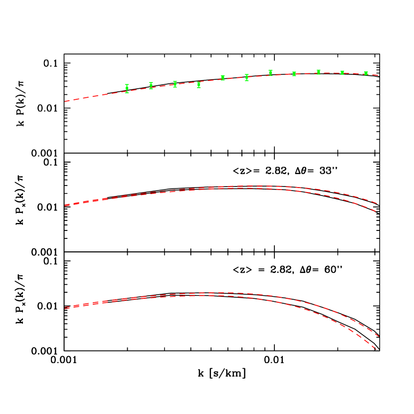
Figure 10: The top panel shows Croft’s measured auto spectrum, interpolated to $\langle z\rangle=2.82$ (green points with error bars), a fit to this with the fitting formula of §6 (red dashed line), and a measurement from simulations (black solid line). The middle panel shows a fit to the cross spectrum at separation $\Delta\theta=33^{\prime\prime}$ (red dashed line), and the simulation measurement at the same separation (black solid line). The top black solid curve in the panel and its red dashed fit are for a $\Omega_{m}=0.3$, $\Omega_{\lambda}=0.7$ (Lambda) cosmology, and the bottom curves for a $\Omega_{m}=1.0$ flat (EDS) cosmology. The bottom panel shows a fit to the cross spectrum at separation $\Delta\theta=60^{\prime\prime}$ (red dashed line) and the simulation measurement at the same separation (black solid line). Again the top curves in this panel are for a Lambda cosmology and the bottom curves for a EDS cosmology.

From the auto and cross spectra measured in this way, we determine the goodness of fit of a model in our parameter grid by calculating, first for the auto spectrum, $\chi^{2}_{\rm auto}=\sum_{i=1}^{n}\left[\frac{\left(P_{\rm sim}(k_{i})-P_{\rm obs}(k_{i})\right)^{2}}{\sigma^{2}_{i}}\right]$. We then compute, as described in §5, the goodness of fit of the model to the observed cross spectrum, using an analogous $\chi^{2}$. We add a term coming from observational constraints on $\langle f\rangle$ to our calculated value of $\chi^{2}_{\rm auto}$. At $z=2.82$ this term is $\chi^{2}=\left[\left(\langle f\rangle-0.682\right)/0.034\right]^{2}$, where the value 0.682 is from Press at al.’s (1993) measurement of the mean transmission, which, at this redshift, is in good agreement with recent measurements by Bernardi et al. (2002) from the SDSS quasar sample, although recently some authors have argued that these measurements may be biased low (Seljak, McDonald & Makarov 2003). The uncertainty in the mean transmission is taken to be $5\%$ following Zaldarriaga et al. (2003). In the equation for $\chi^{2}_{\rm auto}$ the sum runs over the data from Croft et al. (2002) with wavenumber $k_{i}\lesssim 0.03$ s/km, interpolated to $z=2.82$. Here $P_{\rm obs}(k_{i})$ is the observed auto spectrum at wavenumber $k_{i}$, $\sigma_{i}$ is Croft et al.’s (2002) observational error estimate for $P_{\rm obs}(k_{i})$, and $P_{\rm sim}(k_{i})$ is the simulation measurement interpolated to $k=k_{i}$. A resolution test shown in Appendix A demonstrates that our fiducial simulation, with $256^{3}$ particles in a $20.0$ Mpc/h box, gives a reliable (compared with present observational errors) flux auto spectrum on large scales, but misses some power in the auto spectrum on small scales. Because of this, we do not include the auto spectrum data at $k\gtrsim 0.03$ s/km in constructing our fits. (A plot of the auto spectrum is shown later in the text, in figure 10.)

From now on, whenever we refer to the fiducial model for the purpose of illustration, it refers to the following: $(a,n,k_{f},T_{0},\alpha,\langle f\rangle)=(0.19,0.7,35.0$ h^-1 Mpc, $250$ (km/s)², $0.2,0.684)$. Similar models were found to fit the observed auto spectrum by Zaldarriaga et al. (2001a,2003). The power spectrum normalization and slope of this model can also be characterized by $\Delta^{2}(k_{p},z=2.82)$ and $n_{\rm eff}$, which are the amplitude and slope of the linear power spectrum at $k_{p}=0.03$ s/km, $z=2.82$ (Croft et al. 2002). This model has $\Delta^{2}(k_{p},z=2.82)=0.44$, $n_{\rm eff}=-2.7$. The fit has $\chi^{2}_{\rm auto}=6.7$. The model has roughly 4 free parameters, $a,n,T_{0}$, and $\alpha$, since $k_{f}$ and $\langle f\rangle$ are fixed, and we fit to 11 data points, so there are 7 degrees of freedom. The fit, with $\chi^{2}$ per degree of freedom of $0.96$ is reasonable.

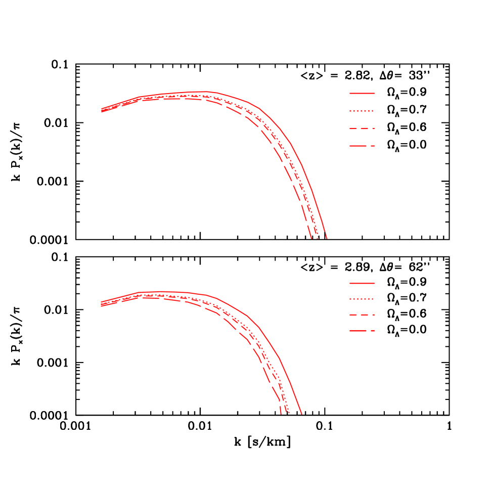
Figure 2: The cross spectrum for a range of flat cosmologies at $\langle z\rangle=2.82,2.89$, assuming a model of the IGM that provides a reasonable fit to the observed auto spectrum at each redshift. The top panel shows the cross spectrum for a separation of $\Delta\theta=33^{\prime\prime}$ and the bottom panel shows the cross spectrum for a separation of $\Delta\theta=62^{\prime\prime}$. These redshifts and separations correspond to those in the data set considered in §5.

Since this fiducial model of the IGM provides a reasonable fit to the observed auto spectrum it is interesting to examine the cross spectra this model predicts for a range of cosmological geometries. From equation (1) we know how different the squashing factors in different cosmologies are, but have yet to examine how different the cross spectra are in these cosmologies. After all, the cross spectrum is the observationally relevant quantity in our study. We illustrate the difference in figure (2) for $\langle z\rangle=2.82,\Delta\theta=33^{\prime\prime}$ and for $\langle z\rangle=2.89,\Delta\theta=62^{\prime\prime}$, which correspond to the redshift and angular separation of two of the pairs we analyze in §5. The cross spectra shown in the figure are estimated from the average of 5 different simulation realizations. These predictions include the effect of redshift distortions as discussed below in §4. Looking first at the $\Delta\theta=33^{\prime\prime}$ plot, it will clearly be difficult to discriminate between a flat $\Omega_{\Lambda}=0.7$ cosmology and a flat $\Omega_{\Lambda}=0.6$ cosmology, as already implied by the similarity of the squashing factor for these two cosmologies in figure (1). At $k_{\parallel}=3.2\times 10^{-3}$ s/km, which is twice the wavenumber at the fundamental mode, the cross spectrum in the $\Omega_{\Lambda}=0.7$ cosmology only differs from the cross spectrum in an EDS cosmology by $\sim 7\%$, while the cross spectrum in the $\Omega_{\Lambda}=0.6$ cosmology differs from the EDS case by only $\sim 5.5\%$. By $k_{\parallel}\sim 0.03$ s/km, the fractional differences with the EDS case are larger, around $\sim 33\%$ for $\Omega_{\Lambda}=0.7$ and $\sim 27\%$ for $\Omega_{\Lambda}=0.6$. However a cosmology with a significant cosmological constant makes its presence felt, and there is a sizeable difference between a flat, $\Omega_{\Lambda}=0.9$ cosmology and a flat, $\Omega_{\Lambda}=0.7$ cosmology. The fractional difference between the $\Omega_{\Lambda}=0.9$ case and the EDS case is $\sim 14\%$ at $k_{\parallel}=3.2\times 10^{-3}$ s/km, and $\sim 53\%$ by $k_{\parallel}\sim 0.03$ s/km. Looking now at the $\Delta\theta=62^{\prime\prime}$ plot, the difference between models is larger, but the magnitude of the cross spectrum is reduced slightly and the scale at which the cross spectrum turns over moves to lower $k_{\parallel}$. At this separation, the fractional difference between the $\Omega_{\Lambda}=0.9$ case and the EDS case is $\sim 21\%$ at $k_{\parallel}=3.2\times 10^{-3}$ s/km and $\sim 73\%$ by $k_{\parallel}\sim 0.03$ s/km. As we describe in §6, however, the ability to discriminate between two cosmologies depends not on the fractional difference between the cross spectra in the two models, but rather on the difference between the cross spectra, divided by the square root of the sum of the squares of the true auto and cross spectra. This means that the discriminating power is actually better for the close separation, $\Delta\theta\lesssim 1^{\prime}$, pairs. However, as we will flesh out in §6, the advantage provided by observing close separation pairs is nullified if the spectral resolution is not good enough to resolve the small scales where such models differ significantly. One can see some noise in the simulation measurement from the $\Delta\theta=62^{\prime\prime}$ pairs at high $k$. Simulation measurements of the cross spectrum at large separations and high $k$ are generally rather noisy. This is not too much of a concern for our present purposes since in this paper we consider an observational data set of relatively close pairs, with poor spectral resolution, confining our measurements from data to large scales. In §6, however, we consider the expected cross spectrum signal at large separations, extrapolating our simulation measurements to these separations using the fitting formula proposed by McDonald (2003).

4 The Flux Power Spectrum and its Redshift Distortion

In order to use the AP test to determine the cosmological constant, we must take into account the effect of redshift distortions. It is our aim in this section to investigate the relative importance of cosmology versus redshift distortions in determining the anisotropy of the observed power spectrum. It is important to emphasize that while we will make comparisons between simulations and linear theory predictions, we will not make use of the linear predictions in the rest of the paper.

The detailed form of the full three-dimensional flux power spectrum involves non-linear effects, the effects of peculiar velocities and of thermal broadening. A start towards understanding these effects was made by Hui (1999), (see also McDonald & Miralda-Escudé 1999), who made a linear theory calculation of the effect of redshift distortions and found that $P_{F}(k,\mu)\propto(1+\beta\mu^{2})^{2}e^{-\frac{k^{2}\mu^{2}}{{k_{s}}^{2}}}P(k)$. (Further investigations have been carried out by McDonald 2003). Here $\mu$ refers to the ratio of the component of the wavenumber along the line of sight, $k_{\parallel}$, to the total wavenumber, $k$. The optical depth is assumed to go as $\tau\propto(1+\delta)^{\nu}$ before the effects of thermal broadening and redshift distortions are included; $P(k)$ is the mass power spectrum in real space; and $\beta=f_{g}(\Omega_{m},z)/\nu$. Here $f_{g}\equiv dlnD/dlna$ is the logarithmic derivative of the linear growth factor, $D(a)$, and $f_{g}(\Omega_{m},z)\sim\Omega_{m}(z)^{0.6}$ for Lambda cosmologies. On large scales $P_{F}(k,\mu)$ has the same qualitative form as the expression for the galaxy power spectrum in redshift space predicted by Kaiser (1987); the three-dimensional flux power is enhanced along the line of sight in redshift space. Here, however, the “bias factor” in the expression is given by $\nu$, the power law in the relation between density and optical depth. On small scales the flux power spectrum is suppressed along the line of sight, as described by the factor $e^{-\frac{k^{2}\mu^{2}}{{k_{s}}^{2}}}$. In linear theory the smoothing scale, $k_{s}$, is the thermal broadening scale, $k_{s}=\sqrt{2}/\sqrt{(T_{0})}$, where $T_{0}$ is the temperature at mean density in units of (km/s)². In the non-linear regime the flux power spectrum will be suppressed on small scales not only from thermal broadening, but also from non-linear peculiar velocities and the suppression will not generally be well described by a Gaussian. This suppression of power is analogous to the finger of god effect found in the case of the galaxy power spectrum in redshift space, but here the effect is due not only to peculiar velocities but also to thermal broadening. In this section we quantify the anisotropy due to redshift distortions by direct measurement from simulations.

We measure the three-dimensional flux power spectrum from a $512^{3},20.0$ Mpc/h simulation, assuming the fiducial model described in the last section. To measure the full three-dimensional flux power spectrum, we form the flux field at every pixel in the simulation box taking the line of sight along one of the box axes, form the power spectrum by three-dimensional FFT, then repeat the measurement with the lines of sight along the other box axes, and average the results over the three box axes.

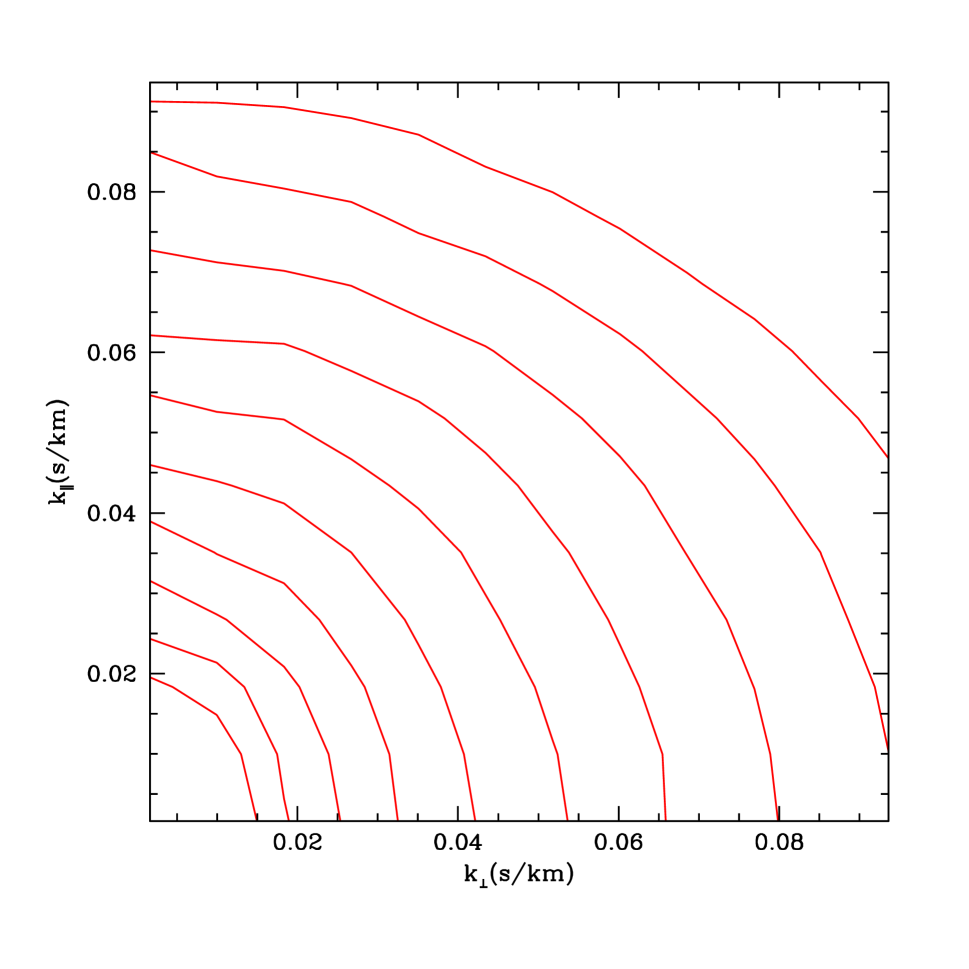
Figure 3: Contours of constant flux power in the $k_{\perp}-k_{\parallel}$ plane. The contours range from ln(P/(km/s)³) = 6.5 to ln(P/(km/s)³)=12.5. The flux power is measured from an SCDM simulation with $512^{3}$ particles in a $20.0$ Mpc/h box. The flux generation parameters are $(a,n,k_{f},T_{0},\langle f\rangle,\alpha)=(0.19,0.7,35.0$ h Mpc^-1, $300$ (km/s)², $0.684,0.1)$

Our measurement is illustrated in figure (3) where we show contours of constant flux power in the $k_{\perp}-k_{\parallel}$ plane. On large scales (small $k$) the contours of constant flux power have a slightly prolate shape. This means that in configuration space contours of constant correlation function would have a slightly oblate shape, signifying a squashing along the line of sight. This behavior, of the flux correlation function in redshift space, is qualitatively the same as the behavior of the galaxy correlation in redshift space; both are squashed on large scales from gravitational infall. At higher $k$, near $k\sim 0.05$ s/km, the situation reverses itself and the contours of constant flux power become oblate, signifying a finger-of-god elongation along the line of sight. This behavior is also exactly analogous to the behavior of the galaxy redshift space power spectrum and is qualitatively consistent with the predictions of Hui (1999), McDonald & Miralda-Escudé (1999), and McDonald (2003).

A useful statistic to quantify the measured anisotropy of the flux power spectrum is its quadrapole to monopole ratio $Q(k)$, as is often done for the galaxy power spectrum in redshift space. (See e.g., Cole, Fisher & Weinberg 1994, Hatton & Cole 1998, Scoccimarro, Couchman & Frieman 1999.) To compute this quantity one writes the anisotropic flux power spectrum, $P_{F}(k,\mu)$, as a sum of Legendre polynomials. The Legendre sum is $P_{F}(k,\mu)=\sum_{l=0}^{\infty}a_{l}(k)L_{l}(\mu)$, where $L_{l}(\mu)$ are the Legendre polynomials, and we wish to determine the coefficients, $a_{l}(k)$, in the expansion. Using the orthogonality of the Legendre polynomials we then have the quadrapole to monopole ratio,

$$Q(k)=\frac{a_{2}(k)}{a_{0}(k)}=\frac{5/2\int_{-1}^{1}d\mu{1\over 2}\left(3\mu^{2}-1\right)P_{F}(k,\mu)}{1/2\int_{-1}^{1}d\mu P_{F}(k,\mu)}$$ (4)

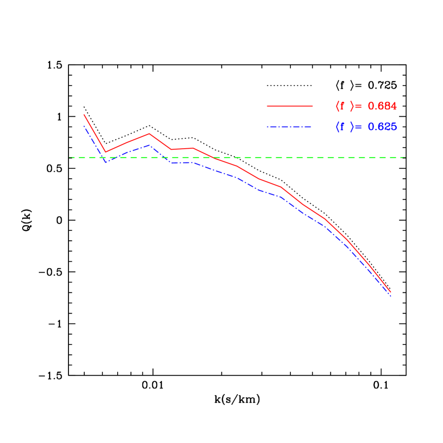
Figure 4: The quadrapole to monopole ratio of the flux power spectrum. The red solid line is a simulation measurement with the same parameters as in figure (3). The simulation measurement is shown starting from $k=3.0\times k_{\rm fundamental}$. The green dashed line is the large scale linear theory prediction, which ignores the finger-of-god effect on small scales. We also show the quadrapole to monopole ratio for two models, identical to the above model, except with differing values of the mean transmission, $\langle f\rangle$, demonstrating the sensitivity of the measurement to $\langle f\rangle$. Note that only the model with $\langle f\rangle=0.684$ provides a good fit to the auto spectrum.

We have measured the quadrapole to monopole ratio at $z=2.82$ assuming the same IGM model parameters as above. A plot of the measurement is shown as the red solid line in figure (4). The measurement is shown starting from three times the fundamental mode, $k=3.0\times k_{\rm fun}$, since on larger scales there are few $k$ modes with which to estimate the anisotropy. The measurement is generally noisy since it comes from only one simulation realization. The measured quadrapole to monopole ratio has the approximate form expected given Hui’s (1999) linear theory calculation. From the linear theory form of the flux power spectrum, one expects that on scales where thermal broadening is negligible, $Q(k)=\frac{4\beta/3+4\beta^{2}/7}{1+2\beta/3+\beta^{2}/5}$. At small $k$, the quadrapole to monopole measurement from the simulation is positive and has approximately the linear theory magnitude, but it appears to be slightly larger on the largest scales measured. On smaller scales, the quadrapole to monopole goes negative due to the suppression of power along the line of sight from the combined effects of peculiar velocities and thermal broadening.

We caution, however, that the quadrapole to monopole ratio is somewhat sensitive to $\langle f\rangle$, which in turn is sensitive to small scale physics, some of which may be missing from our relatively low resolution, N-body simulations. It is not obvious that the linear theory calculation gives the correct biasing factor, as Hui (1999) points out. As Hui (1999) emphasizes, the redshift distortions of the flux power spectrum are complicated, involving several transformations; a transformation from gas density to neutral hydrogen density, a transformation of the optical depth into redshift space involving both a shift by peculiar velocity and convolution with a thermal broadening window, and finally an exponentiation to go from optical depth to flux. The effect then of small scale, non-linear behavior on the redshift distortions at large scales is not clear. We know, at any rate, that small scale physics is important in determining $A$ (the parameter adjusted to match the observed mean transmission discussed in §3.1), which in turn affects the large scale flux power. It is perhaps not terribly surprising then that the quadrapole to monopole depends somewhat on $\langle f\rangle$, since this parameter sets which range of mass overdensities the flux field, $\delta_{f}$, is sensitive to. The black dotted and blue dot-dashed lines in figure (4) show the quadrapole to monopole ratios for models with $\langle f\rangle=0.625,0.725$, illustrating the dependence on $\langle f\rangle$. The quadrapole to monopole ratio for the model with the largest $\langle f\rangle$ is a bit larger than the fiducial model while the model with the smallest $\langle f\rangle$ has a smaller quadrapole to monopole ratio than the fiducial model. This means that the quadrapole to monopole ratio is likely to have a different magnitude at different redshifts, where the mean transmission is different. Indeed the fitting formula that McDonald (2003) found (see §6) for the three dimensional flux power spectrum at $\langle z\rangle\sim 2.25$ implies a somewhat larger quadrapole to monopole ratio on large scales, which is qualitatively consistent with our expectations given the larger mean transmission at that redshift. After performing these measurements and making the caveat about the dependence of our results on $\langle f\rangle$, we leave a more systematic investigation of flux power redshift distortions for future work.

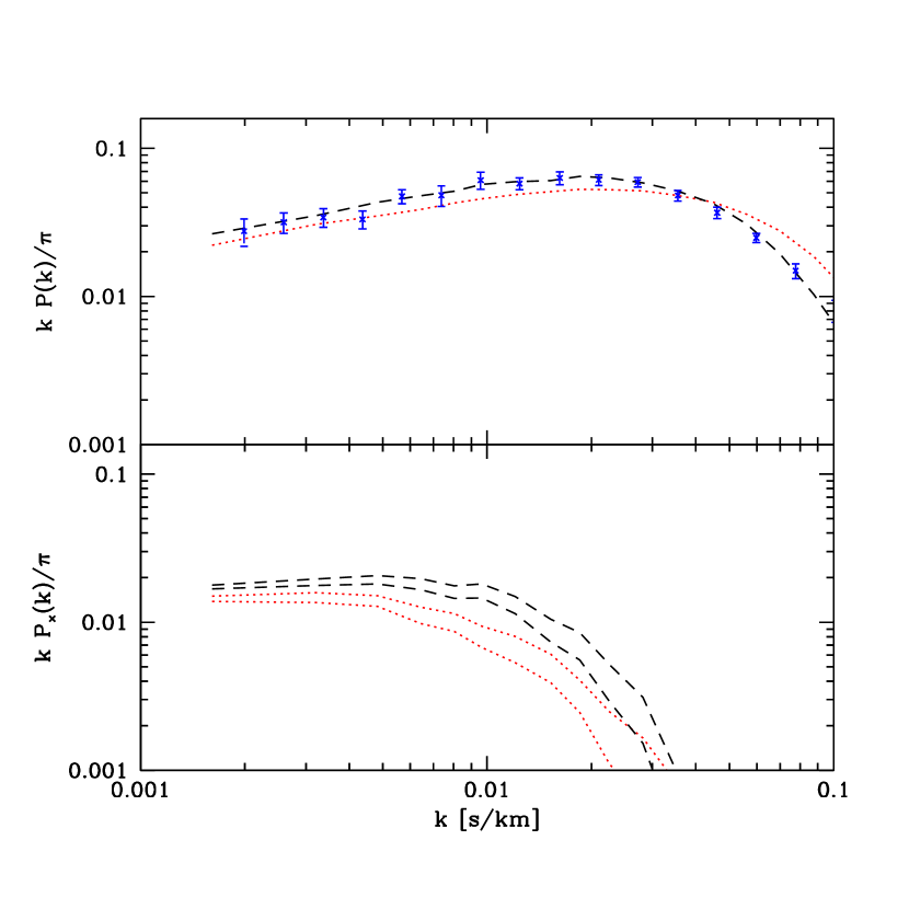
Figure 5: The top panel shows (black dashed line) the auto spectrum from the $512^{3}$ simulation including the effects of thermal broadening and peculiar velocities. The red dotted line is the auto spectrum in the same model, without the effect of peculiar velocities and thermal broadening. The blue points with error bars are Croft et al’s (2002) measurement interpolated to $\langle z\rangle=2.82$. The bottom panel shows (black dashed lines) the cross spectrum measured at $\Delta\theta=60^{\prime\prime}$ measured in a Lambda model (top black dashed line) and in a EDS model (bottom black dashed line). The red dotted lines are the cross spectra measured in the same models, ignoring the effect of redshift distortions. In calculating the cross spectra in the redshift distortion free case, the mass power spectrum amplitude of the model has been adjusted so that the corresponding auto spectrum matches observations on large scales.

Given these measurements of the anisotropy of the three-dimensional flux power spectrum due to redshift distortions, it is natural to ask how large the anisotropy from redshift distortions is in comparison to the anisotropy from cosmological distortions. To gauge the relative size of the two effects we consider the power spectrum of $f=e^{-A(1+\delta)^{\nu}}$; the flux power spectrum neglecting thermal broadening and peculiar velocities, which is isotropic. We refer to this field as the isotropic flux field to distinguish it from the anisotropic flux field that includes redshift distortions. In the top panel of figure (5) we show a comparison of the auto spectrum measured from the fully anisotropic flux field and that measured from the isotropic flux field for the same model of the IGM. On large scales, the auto spectrum measured from the anisotropic flux field is boosted compared to that measured from the isotropic flux field. On the other hand, on small scales the auto spectrum measured from the anisotropic flux field is suppressed relative to that measured from the isotropic flux field. This qualitative behavior of the auto spectrum, that redshift distortions boost the auto spectrum on large scales and suppress the auto spectrum on small scales is expected from our above measurements of the full three-dimensional flux power. How different then our the cross spectra of the isotropic flux field and the anisotropic flux field? To provide a fair comparison, we first boost the mass power spectrum normalization in the isotropic case so that the auto spectrum of the isotropic flux field matches the observed auto spectrum on large scales ($k\lesssim 0.03$ s/km). The corresponding cross spectra are shown in the bottom panel of figure (5) for lines of sight separated by $\Delta\theta=60^{\prime\prime}$ in each of a Lambda ($\Omega_{\Lambda}=0.7$) cosmology and an EDS cosmology. From the figure, one can see that redshift distortions significantly boost the amplitude of the cross spectrum in each cosmology. If one naively neglects redshift distortions, the cross spectrum one predicts in the Lambda cosmology (top red dotted line) is less than that of the cross spectrum in the EDS cosmology including redshift distortions (bottom black dashed line)! At larger separations, we expect that the geometrical effect will become more important relative to the effect of redshift distortions. At any rate, this clearly suggests that redshift distortions are an important effect and must be accounted for in detail in order to apply the Ly$\alpha$ AP test. Now that we have some sense of the size of the cosmological distortion and the size of the redshift distortions, we measure the cross spectrum from a small data sample.

5 Measurements of the Cross Power Spectrum from a sample of Close Quasar Pairs

In this section we present both a measurement of the cross spectrum from our data, and present constraints obtained from comparison with a small grid of simulated models. In Table (1) we provide a summary of pertinent information for the quasar pairs that we analyze. Observations were performed with the 4-meter/RC spectrograph combination at both Kitt Peak National Observatory and Cerro Tololo Inter-american Observatory, using the T2KB CCD detector and grating BL420 in 2nd order, and the Loral 3K CCD and KPGL1 grating (1st order), respectively, delivering 3150Å$\lesssim\lambda\lesssim 4720$Å and 3575Å$\lesssim\lambda\lesssim 6675$Å for the KP triplet and 2139-44/45 pairs, respectively. Further details of these (and redder observations for the KP triplet, plus further spectra for additional objects) are detailed in Crotts & Bechtold (2003).

In order to estimate the cross spectrum of a given quasar pair the following procedure is followed:

• We extract the region of the Ly$\alpha$ forest that is common to each member of a quasar pair, avoiding regions close to each quasar that might be contaminated by the proximity effect. (Bajtlik et al. 1988) We make a conservative cut for the proximity effect, including only the region in the Ly$\alpha$ forest corresponding to rest frame wavelengths of $\lambda_{\rm rest}\sim 1051$Å$-1185$Å. We then discard regions that do not overlap in wavelength between each member of a given pair. In the case of the KP triplet, we discard regions that do not overlap across the entire triplet.

  We have not made any attempt to remove metal absorption lines in the Ly$\alpha$ forest. The effect of metal lines on the flux power spectrum is expected to be small, except on scales smaller than the resolution of our present data (McDonald et al. 2000).

• We determine the flux field, $\delta_{f}=(f-\langle f\rangle)/\langle f\rangle$, for each member of a quasar pair. Here $f$ is the flux at a given pixel and $\langle f\rangle$ is the mean flux. To do this we follow the procedure of Croft et al. (2002). We smooth the entire spectrum with a large radius, $50$ Å, Gaussian filter giving the smoothed number of counts, $f_{s}(\lambda)$, as a function of wavelength. From the smoothed spectrum, $\delta_{f}$ is given by $\delta_{f}=\left(f(\lambda)-f_{s}(\lambda)\right)/f_{s}(\lambda)$. This procedure estimates the mean flux directly, avoiding a measurement of the unabsorbed continuum level. Clearly, however, this procedure does not allow one to reliably measure the flux power on scales $r\gtrsim 50$ Å, but the flux power on these scales is expected to be contaminated by continuum fluctuations anyway (Zaldarriaga et al., 2001b). We confine ourselves to measurements of cross power on scales of $k_{\parallel}\gtrsim 2.0\times 10^{-3}$ s/km.

• We estimate the cross spectrum from the following estimator, utilizing 1d FFTs:

  $$\hat{P}_{\times}(k_{\parallel},\Delta\theta)=\frac{1}{n_{k}}\sum_{i=1}^{n_{k}}\frac{1}{2}\left[\delta_{a}(k_{i})\delta^{*}_{b}(k_{i})+\delta_{b}(k_{i})\delta^{*}_{a}(k_{i})\right]$$ (5)

  Here the sum is over the $n_{k}$ modes in a given k-bin, $k_{i}$ is the ith mode in the bin, and $k_{\parallel}$ is the average wave number in the bin. Our convention is that modes with $|k_{i}|$ and $-|k_{i}|$ fall within the same k-bin and that $k_{\parallel}$ is always positive, so that $|k_{i}|$ and $-|k_{i}|$ count as two modes towards $n_{k}$. The Fourier amplitude $\delta_{a}(k_{i})$ comes from the Fourier transform of the flux field of the first spectrum in the pair, $\delta_{b}(k_{i})$ from the Fourier transform of the second spectrum in the pair and $\delta^{*}_{a}$, $\delta^{*}_{b}$ are their complex conjugates. The cross spectrum is thereby a real quantity that contains information about the relative phase of the Fourier coefficients, $\delta_{a}(k_{i})$, $\delta_{b}(k_{i})$, as well as their amplitude.

• An estimate of the error on the cross spectrum measurements is made assuming Gaussian statistics, a procedure which seems to be supported on relevant scales by analyses from a large number of spectra from the SDSS (Hui et al., in preparation). With this assumption the error on the cross-spectrum estimate is (see Hui et al. 2001 for a derivation of the auto-spectrum variance)

  $$\sigma_{\hat{P}}^{2}(k_{\parallel})=\frac{1}{n_{k}}\left[\left(P_{\times}(k_{\parallel},\Delta\theta)\right)^{2}+\left(P_{\rm 1d}(k_{\parallel})+b^{a}(k_{\parallel})\right)\left(P_{\rm 1d}+b^{b}(k_{\parallel})\right)\right]$$ (6)

  Here $P_{\rm 1d}(k_{\parallel})$ and $P_{\times}(k_{\parallel},\Delta\theta)$ refer to the true auto and cross spectra as opposed to the noisy estimates from the data, which we refer to as $\hat{P}_{\rm 1d}$ and $\hat{P}_{\times}$. In the above equation $b^{a}(k_{\parallel})$ and $b^{b}(k_{\parallel})$ are estimates of the shot-noise in each spectrum. As in equation (5), $k_{\parallel}$ refers to the average wavenumber in a $k$-bin and $n_{k}$ is the number of modes in the bin counted with the convention described previously. When using these equations to estimate the error on the cross spectrum, we use simulation measurements to provide the true auto spectrum, $P_{\rm 1d}(k_{i})$ and the true cross spectrum, $P_{\times}(k_{i},\Delta\theta)$. The simulation measurements are made assuming a model for the IGM that fits the observed auto spectrum at the relevant redshift. For the purposes of computing the error, we assume an $\Omega_{m}=0.3$, $\Omega_{\Lambda}=0.7$ cosmology. For pairs with large separations, the cross spectrum contribution to the error is negligible. In practice we measure the cross power of spectra that are smoothed by the limited spectral resolution of the observations, and so we take $\sigma_{\hat{P}}(k_{\parallel})\to\sigma_{\hat{P}}(k_{\parallel})W(k_{\parallel})$, where $W(k_{\parallel})$ describes the smoothing due to limited spectral resolution.

• In deriving a constraint on $\Omega_{\Lambda}$ from the KP triplet, we need to take into account that each pair is not independent of the other pairs. A given pairing of lines of sight from the triplet has a line of sight in common with every other pairing and so measurements of the cross spectrum at a given scale are correlated across the different pairs. To take this correlation into account, we consider the covariance between cross spectrum measurements from two pairs that have a line of sight in common. Assuming Gaussian statistics, and ignoring shot-noise which should be unimportant on the scales we probe reliably with the KP triplet, we find that the covariance is

  $$\langle\delta P_{\times}^{12}(k_{\parallel},\Delta\theta)\delta P_{\times}^{23}(k_{\parallel},\Delta\theta^{\prime})\rangle=\frac{1}{n_{k}}\left[P_{\times}^{12}(k_{\parallel},\Delta\theta)P_{\times}^{23}(k_{\parallel},\Delta\theta^{\prime})+P_{1d}(k_{\parallel})P_{\times}^{13}(k_{\parallel},\Delta\theta^{\prime\prime})\right]$$ (7)

  The lines of sight are labeled by $1$, $2$, and $3$. We write down the expression for the covariance between cross spectrum estimates of pairs $12$ and $23$, so that line of sight $2$ is the common line of sight to the two pairs, expressions for other pairings follow from swapping the super-scripts. In this equation $P_{\times}^{12}(k_{\parallel},\Delta\theta)$ is the cross spectrum of lines of sight 1 and 2, which are separated by an angle $\Delta\theta$, $P_{\times}^{23}(k_{\parallel},\Delta\theta^{\prime})$ and $P_{\times}^{13}(k_{\parallel},\Delta\theta^{\prime\prime})$ have similar meanings, $P_{1d}(k_{\parallel})$ is the auto spectrum, and $k_{\parallel}$, $n_{k}$ have the meanings described above.

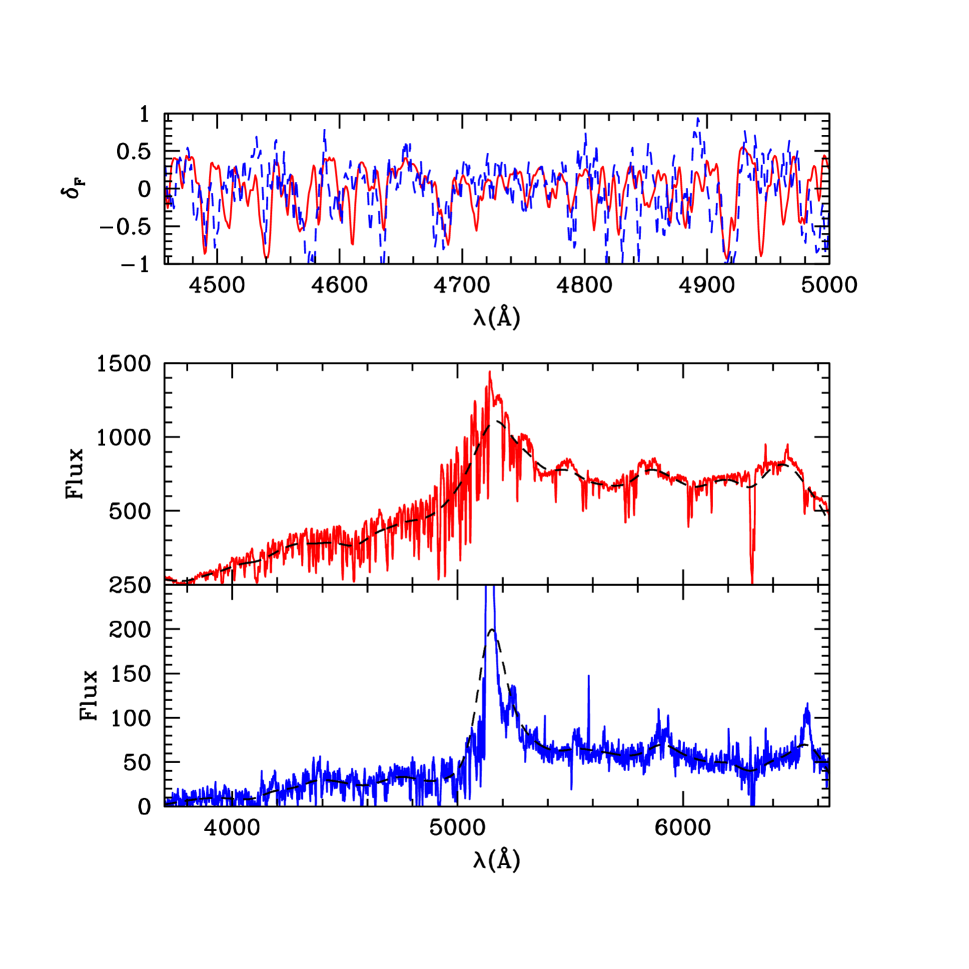
Figure 6: The bottom panel shows the spectrum of Q2139-4433 (red solid line) and the middle panel shows the spectrum of Q2139-4434 (blue solid line). The dark dashed lines show the spectra when smoothed with a Gaussian filter of $50\AA$ radius in order to form $\delta_{F}$ (see text). The top panel shows $\delta_{F}$ overlayed for each spectrum. The red solid line is $\delta_{F}$ for Q2139-4433 and the blue dashed line is Q2139-4434. The pair is separated by $\Delta\theta=62^{\prime\prime}$.

In figure (6) we provide an example of our procedure for forming $\delta_{f}$. The spectra of the members of the pair Q2139-33/34 are shown, as well as the result of smoothing them with a $50\AA$ filter. The flux fields, $\delta_{f}$, are shown one on top of the other, with the above cuts for the proximity effect. One can visually discern a cross-correlation between the two spectra in this pair, which has a separation of $62^{\prime\prime}$. We generate flux fields for the other pairs in a similar fashion.

We then compare our measurements with a grid of models, using the method of Zaldarriaga et al. (2001a,2003). In particular for each of the two high redshift pairs we generate models with
$a=(0.11,0.14,0.19,0.24)$, $n=(0.7,0.8,0.9,1.0)$, $k_{f}=35.0$ h Mpc^-1, $T_{0}=(200,250,300)$ (km/s)²,
$\alpha=(0.0,0.2,0.4,0.6)$, $\langle f\rangle=(0.625,0.666,0.700)$ at $\langle z\rangle=2.89$ and $\langle f\rangle=(0.650,0.684,0.725)$ at $\langle z\rangle=2.82$, $\Omega_{\Lambda}=(0.0,0.1,0.2,0.3,0.4,0.5,0.6,0.7,0.8,0.9,1.0)$. At $\langle z\rangle=2.26$, our grid spans a different range of power spectrum normalizations, $a=(0.24,0.27,0.31)$ and mean transmissions, $\langle f\rangle=(0.750,0.800,0.850)$. In computing the likelihood of each model in the grid, as described in §3.1, we include a prior constraint on $\langle f\rangle$. This constraint is $\langle f\rangle=0.666\pm 0.033$ at $\langle z\rangle=2.89$, $\langle f\rangle=0.682\pm 0.034$ at $\langle z\rangle=2.82$, and $\langle f\rangle=0.802\pm 0.040$ at $\langle z\rangle=2.26$. The values of $\langle f\rangle$ come from the measurements of Press et al. (1993). In comparing the theoretical predictions with the observed auto spectrum, since we compare with only one simulation realization, we do not include points with $k\lesssim 2\times k_{\rm fun}$ where $k_{\rm fun}$ is the fundamental mode of the simulation box (see Appendix A). We do include such points in our cross spectrum analysis because the observational error bars on these points are very large and our results are not very sensitive to whether we include these points or not.

For each model in our grid, we then compute $\chi^{2}_{\rm tot}=\chi^{2}_{\rm auto}+\chi^{2}_{\rm cross}$. The computation of $\chi^{2}_{\rm auto}$, the goodness of fit of the model auto spectrum to the observed auto spectrum of Croft et al. (2002) interpolated to the relevant redshift, is described in §3.1. To compute $\chi^{2}_{\rm cross}$ we take the sum $\chi^{2}_{\rm cross}=\sum_{i=1}^{n}\left[\frac{(\widetilde{P}_{\rm\times,sim}(k_{i},\Delta\theta)-P_{\rm\times,obs}(k_{i},\Delta\theta))^{2}}{\sigma^{2}_{i}}\right]$. Here $P_{\rm\times,obs}(k_{i},\Delta\theta)$ is the observed cross spectrum measurement at wavenumber $k_{i}$ and transverse separation $\Delta\theta$, $\widetilde{P}_{\rm\times,sim}(k_{i},\Delta\theta)$ is the simulation measurement linearly interpolated to the same $k_{i}$ and $\Delta\theta$, and smoothed to mimic the limited spectral resolution of our cross spectrum measurement. The error estimates of 6 and 7 are multiplied by the smoothing window before calculating $\chi^{2}$. The spectral resolution of each spectrum is shown in Table (1). We truncate the sum at $k_{n}$, the scale at which the limited spectral resolution causes the measured cross power to drop to $50\%$ of the value it would have with perfect resolution. From the vales of $\chi^{2}_{\rm tot}$ at each point in the parameter grid we determine marginalized constraints on $\Omega_{\Lambda}$ following the method of Tegmark & Zaldarriaga (2000), Zaldarriaga et al. (2001a,2003).

In brief, the method of Tegmark & Zaldarriaga (2000) is as follows. We begin from a grid of $\chi^{2}$ points in a seven-dimensional parameter grid. We wish to find constraints on $\Omega_{\Lambda}$, marginalized over all of the other “nuisance” parameters in the grid. To do this one should integrate over the “nuisance” parameters. In this paper, we avoid the full multidimensional integration by assuming that the likelihood function is multi-variate Gaussian, in which case integrating out a parameter is equivalent to maximizing the likelihood over the parameter (Tegmark & Zaldarriaga 2000). We then maximize over each parameter in turn, first cubic spline-interpolating over the parameter. In this way we obtain marginalized constraints on $\Omega_{\Lambda}$.

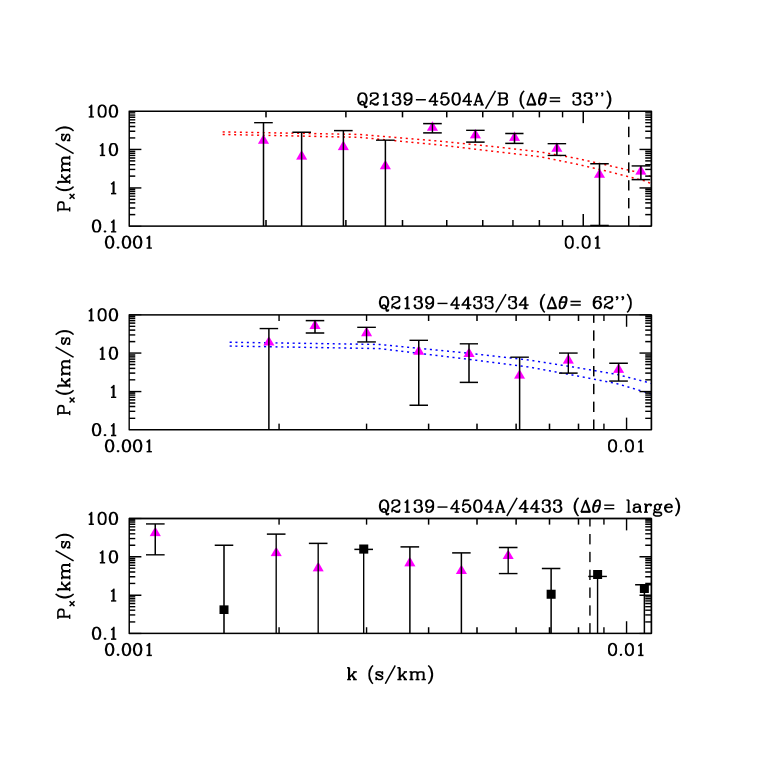
Figure 7: The top panel shows the cross spectrum measured from the pair Q2139-4504A/B. We also show models from our grid that are close to the best fit, (to the combined auto and cross spectra), flat universe models with $\Omega_{\Lambda}=0.9$ (top curve) and $\Omega_{\Lambda}=0.0$ (bottom curve). (Since $\chi^{2}$ is spline interpolated between grid points, the minimum value we obtain for $\chi^{2}$ does not occur precisely on a grid point in the parameter space. The curves shown are thus at grid points close to this true minimum.) The model fits have been multiplied by a filter representing the limited spectral resolution of the observations. The dashed line indicates the cut we make on the data due to the limited spectral resolution; only points to the left of the dashed line are included in our fit. The other IGM parameters are the same for both models, $(a,n,k_{f},T_{0},\langle f\rangle,\alpha)=(0.19,0.8,35,200,0.684,0.4)$. The models in the top panel are somewhat poor fits to the observed cross spectrum, which has more power on small scales. The middle panel shows the same for the pair Q2139-4433/34. In this case the other IGM parameters are $(a,n,k_{f},T_{0},\langle f\rangle,\alpha)=(0.14,0.9,35,250,0.666,0.0)$. and the models provide reasonable fits to the measured cross spectrum. The bottom panel shows the cross spectrum of a widely separated pair, which is consistent with zero. The magenta diamonds indicate points with a positive cross spectrum and the black squares indicate the absolute value of points with a negative cross spectrum.

The cross spectrum measurements from the two high redshift pairs are shown in the top two panels of figure (7). From the figure one sees that the signal is generally weakly detected on large scales where few modes are available. On these scales some of the measurements in different k bins are consistent with zero at the $1\sigma$ level. A more significant signal is detected on small scales where more modes are available. Before comparing these cross spectrum measurements with models from the simulation grid, it is useful to measure the cross spectrum from the overlapping regions in the Ly$\alpha$ forests of a widely separated quasar pair. If our underlying assumption that the cross spectrum signal arises from fluctuations in the underlying density field is correct, the cross spectrum of widely separated pairs should be consistent with zero. In the bottom panel of figure (7) we show a measurement of the cross spectrum between the spectra of Q2139-4504A/4433. Over the range of scales that we use here for our constraints, the cross spectrum of the widely separated pair is consistent with zero. Quantitatively, we find that $\chi^{2}$ for the measurement, compared with the null hypothesis of $P_{\times}(k_{\parallel},\Delta\theta=\infty)=0.0$, is $5.0$ for $7$ degrees of freedom.

We then compare the measured cross spectra with fits from the simulation grid. For the pair Q2139-4433/34, at separation $\Delta\theta=62^{\prime\prime}$ and $\langle z\rangle=2.89$, we find that the cross spectrum measurements are fit reasonably well by models from the simulation grid. In particular the minimum $\chi^{2}$ is $\chi^{2}_{\rm tot}\sim 11.2$ obtained near $\Omega_{\Lambda}=0.9$. This is a reasonable fit to the 16 data points considered, (9 auto spectrum points and 7 cross spectrum points), given that our model has roughly 5 free parameters. Each of the auto and cross spectrum are well fit by the model; a model at a nearby grid point in the parameter space has $\chi^{2}_{\rm auto}\sim 5.7$. To gauge the difference between models with different $\Omega_{\Lambda}$ we show models in figure (7) with $\Omega_{\Lambda}=0.9$ and $\Omega_{\Lambda}=0.0$ that are close to the interpolated best fit parameters. We emphasize that $\chi^{2}$ is spline interpolated between grid points and so the minimum value of $\chi^{2}$ does not, in general, lie on a grid point in the parameter space. We include the plots of the model cross spectra just to provide some visual comparison between the data and the model fits. The cross spectrum measurement of the pair Q2139-4504A/B is not as well fit by the models in the parameter grid. The best fit model in the grid has $\chi^{2}_{\rm tot}=15.8$ obtained at $\Omega_{\Lambda}=1.0$. The fit is to 18 data points (9 auto spectrum points and 9 cross spectrum points), with roughly 5 free parameters. The auto spectrum is very well fit for these models with nearby grid points having $\chi^{2}_{\rm auto}\sim 3.5$. The poor $\chi^{2}_{\rm cross}$ for this pair is somewhat surprising. We searched the spectra for contaminating metal line absorbers and for artifacts, but found no effects in the wavelength range we analyze. Another possible issue is that we need to estimate our resolution window carefully, since we have included scales where the power is suppressed by the resolution by $\lesssim 50\%$. We made a careful estimate by looking at the widths of narrow metal lines and night sky lines. For now we consider the poor fit for Q2139-4504A/B to be a curiosity, but point out that larger data samples in the future will allow us to test more carefully for systematic effects.

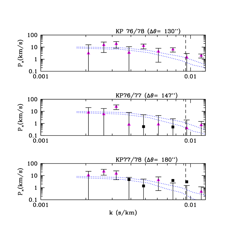
Figure 8: The panels show measurements of the cross spectrum from the KP triplet pairs, as well as models from the simulation grid with $\Omega_{\Lambda}=0.9$ and $\Omega_{\Lambda}=0.0$ to provide some comparison between the data and model fits. The models have $(a,n,k_{f},T_{0},\langle f\rangle,\alpha)=(0.24,0.9,35,250,0.800,0.6)$. The model fits have been multiplied by a filter representing the limited spectral resolution of the observations. The magenta diamonds indicate points with a positive cross spectrum and the black squares indicate the absolute value of points with a negative cross spectrum. In examining this figure, one should keep in mind that the measurements of the cross spectrum at a given scale are correlated across the different pairs, as discussed in the text.

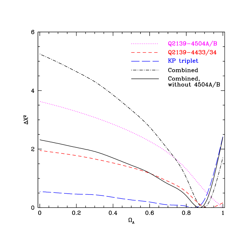
Figure 9: The constraint on $\Omega_{\Lambda}$ from the quasar pairs. The magenta dotted line shows $\Delta\chi^{2}=\chi^{2}-\chi^{2}_{\rm min}$ from the pair Q2139-4504A/B. The red short-dashed line shows the constraint from the pair Q2139-4433 and the blue long-dashed line shows the constraint from the KP triplet. The black dot-dashed line is the combined constraint. The black solid line shows the constraint obtained ignoring Q2139-4504A/B, since the cross spectrum of this pair is somewhat poorly fit by the models in our simulation grid.

In figure (8) we show the measurements obtained from the KP triplet. In this case the cross spectrum signal of the pairs, with $\langle z\rangle\sim 2.26$ and separations in the range of $\Delta\theta\sim 2^{\prime}-3^{\prime}$, is only weakly detected. For the two larger separation pairs most of the measurements of the cross spectrum at different scales are consistent with zero. In spite of this, we still obtain a weak constraint on $\Omega_{\Lambda}$ from the KP triplet, taking into account the covariance between the cross spectrum estimates of the three pairs. The best fit model is obtained near $\Omega_{\Lambda}\sim 0.85$, where $\chi^{2}_{\rm tot}=24.6$. This is a reasonable fit given that there are 21 cross spectrum points and 9 auto spectrum points, and roughly 5 free parameters for a total of 25 degrees of freedom. We then combine the marginalized constraints on $\Omega_{\Lambda}$ by adding the $\chi^{2}_{\rm tot}$ curve from the KP triplet with the constraints from Q2139-4433/34 and Q2139-4504A/B. Given that the cross spectrum of the pair Q2139-4504A/B is somewhat poorly fit by the models in the simulation grid, we also consider the combined constraint ignoring this pair. Including Q2139-4504A/B, the minimum total $\chi^{2}$ for the five pairs is $\chi^{2}_{\rm tot}\sim 52.5$, (for $\sim 59$ degrees of freedom), obtained near $\Omega_{\Lambda}\sim 0.9$. If we don’t include the poorly fit pair, the total $\chi^{2}$ is $\chi^{2}_{\rm tot}\sim 36.1$ for the combined measurement, (for $\sim 41$ degrees of freedom) which occurs near $\Omega_{\Lambda}\sim 0.9$. The result, shown in figure (9), is that, if we include Q2139-4504A/B, $\Delta\chi^{2}=\chi^{2}-\chi^{2}_{\rm min}$ is $\sim 5.1$ for a flat model with $\Omega_{\Lambda}=0$, implying such a cosmology is excluded at the $\sim 2.3\sigma$ level. Ignoring the poorly fit pair, $\Delta\chi^{2}$ reaches $\sim 2.3$ for $\Omega_{\Lambda}=0$. Our small sample of pairs seems to already disfavor an EDS cosmology at a significance of $\sim 1.5\sigma$, or at an even larger significance if one includes the constraint from the poorly fit pair. There is a weak preference from each pair for a high value of $\Omega_{\Lambda}$; models with moderate $\Omega_{\Lambda}\sim 0.6$ are similarly disfavored at the $\gtrsim 1\sigma$ level. Admittedly, even ignoring the poorly fit pair, some our ability to rule out an EDS cosmology comes from just two $k$-bins in the pair Q2139-33/34 with particularly large cross power (see figure 7). While we have no reason to believe the measurements in these $k$-bins are unreliable, we can check how much the significance depends on them. Ignoring these two $k$-bins, we find that an EDS cosmology is still disfavored at the 1$\sigma$ level.

6 Predictions for Future Samples/Observational Strategies

Clearly it is not possible to draw any strong conclusions with the limited sample of five pairs analyzed above. This motivates considering the type of sample necessary to do better in the future. In this section we make predictions for the signal-to noise level (S/N) at which one can distinguish between two different cosmologies with a given number of quasar pairs, and examine the dependence of the expected S/N level on observational resolution and shot noise. We hope that these considerations will be useful in constructing an optimal observing strategy. This is similar to estimates considered in (Hui, Stebbins & Burles 1999), but here we use more accurate expressions for the cross spectrum; our estimates coming from simulations that include the effects of redshift distortions and the detailed form of the three-dimensional flux power spectrum. These authors also limited their considerations to large scales, ($k\lesssim 0.02$ s/km), because of concerns about non-linear effects. We model the non-linear effects with simulations and so can consider the benefit gained from high $k$ modes, which can be quite substantial given close separation pairs and high resolution data. In addition, we consider the effects of instrumental resolution and shot-noise. McDonald (2003) has also made this type of comparison, primarily considering the expected signal from pairs obtained with the SDSS. While our results are broadly consistent with his, we emphasize the potential gain from very close separation pairs observed with high spectral resolution.

The expected signal to noise level at which one can distinguish between two cosmologies with the Ly$\alpha$ AP test is:

$$\frac{S}{N}\sim\left[\frac{fL}{\pi}\int_{k_{\parallel}=k_{\rm min}}^{k_{\parallel}=k_{\rm max}}dk_{\parallel}\left[\frac{P^{A}_{\times}(k_{\parallel},\Delta\theta)-P^{B}_{\times}(k_{\parallel},\Delta\theta)}{\sqrt{\left(P_{\rm 1d}(k_{\parallel})+b(k_{\parallel})\right)^{2}+\left(P^{A}_{\times}(k_{\parallel},\Delta\theta)\right)^{2}}}\right]^{2}\right]^{1/2}$$ (8)

In this equation $P^{A}_{\times}(k_{\parallel},\Delta\theta)$ is the assumed true cross spectrum, and $P^{B}_{\times}(k_{\parallel},\Delta\theta)$ is the cross spectrum in a model we would like to rule out. The denominator is the Gaussian error estimate on the variance of the cross spectrum given in equation (6) for a single $k$-mode. We caution that the Gaussian error estimate is likely to be inaccurate on small scales, but leave a more careful treatment of errors for future work. The integral is over all positive $k$-modes, from the lower limit of $k_{\rm min}$ to the upper limit of $k_{\rm max}$, with a density of states factor of $L/\pi$. For the length of the spectrum we take $L\sim 37,500$ km/s. The factor $f$ is the fraction of the wavelength coverage between Ly$\alpha$ and Ly$\beta$ that is overlapping between the two spectra in the pair, which we take to be $f=1$. The minimum wavenumber in the integral, $k_{\rm min}$ is taken to be $k_{\rm min}=2.0\times 10^{-3}$ s/km since larger scales are expected to be contaminated by fluctuations in the continuum. The maximum wavenumber in the sum is set by the spectral resolution of the observation; it is taken to be the wavenumber where the measured power falls to $1/e$ of its true vales. Modeling the effect of spectral resolution as a Gaussian smoothing, this wavenumber is given by $k_{\rm max}=\frac{1}{\sigma_{s}}$, where $\sigma_{s}$ is related to the instrumental FWHM by $\sigma_{s}=\frac{FWHM}{2\sqrt{2\ln(2)}}$. In considering high spectral resolution data, we enforce an upper limit of $k_{\rm max}=0.1$ s/km, since the Ly$\alpha$ forest is expected to be contaminated by metal lines on such scales (McDonald et al. 2000). One caveat is that in estimating our ability to discriminate between models in this way, we assume perfect knowledge of the other parameters that go into our modeling; the power spectrum normalization, the primordial spectral index, the temperature of the IGM, etc. Measurements of the auto spectrum from SDSS should dramatically reduce the error bars on the observed auto spectrum, and make the associated errors in our modeling parameters smaller. Uncertainties in these modeling parameters will, however, affect our ability to constrain $\Omega_{\Lambda}$, so the constraints quoted below are optimistic. We would like to estimate our ability to discriminate between cosmological models using pairs with a range of separations. Unfortunately, as described in §(3.1), direct measurements of the cross spectrum at large separations from simulations are rather noisy. To get around this difficulty, we use a fitting formula that describes the fully three-dimensional flux power spectrum and reproduces the results of simulation measurements at small separations. This allows us to extrapolate cross spectrum measurements to large angular separations. In particular, at our fiducial redshift of $\langle z\rangle=2.82$, we find the cross and auto spectra are well fit if the three-dimensional flux power spectrum follows the fitting form found by McDonald (2003), $P_{F}(k,\mu)=b_{\delta}^{2}(1+\beta\mu^{2})D(k,\mu)P_{L}(k)$, with $D(k,\mu)=exp\left[\left(\frac{k}{k_{\rm NL}}\right)^{\alpha_{\rm NL}}-\left(\frac{k}{k_{p}}\right)^{\alpha_{p}}-\left(\frac{k_{\parallel}}{k_{v}(k)}\right)^{\alpha_{v}}\right]$ and $k_{\rm v}(k)=k_{\rm v0}(1+k/k^{\prime}_{v})^{\alpha_{v}^{\prime}}$. Here $P_{L}(k)$ is the linear power spectrum of mass and $D(k,\mu)$ describes the effect of non-linear redshift distortions. The first term in $D(k,\mu)$ describes non-linear growth, the second term pressure smoothing, and the third term describes the effect of non-linear peculiar velocities and thermal broadening. The first two terms describe isotropic effects, while the third term has a $\mu$ dependence since thermal broadening and peculiar velocities act only along the line of sight. Given this fitting formula we predict auto and cross spectra by numerical integration using equations (2) and (3). At our fiducial redshift of $\langle z\rangle=2.82$ the cross and auto spectra are fit using the fitting parameters $b_{\delta}^{2}=0.04$, $\beta=0.62$, $k_{\rm NL}=10.0$ h Mpc^-1, $\alpha_{\rm NL}=0.550$, $k_{P}=14.0$ h Mpc^-1, $\alpha_{p}=2.12$, $k_{\rm v0}=5.50$ h Mpc^-1, $\alpha_{v}=1.25$, $k^{\prime}_{v}=0.917$ h Mpc^-1, and $\alpha^{\prime}_{v}=0.528$. These parameters are different than the ones found by McDonald (2003), but he considers a lower redshift, $z=2.25$, and uses a different linear power spectrum model. In figure (10) we show the fits to the auto and cross spectra from simulation measurements. The model fit to the auto spectrum is reasonable. The plot also shows fits at separations of $\Delta\theta=33^{\prime\prime}$ and $\Delta\theta=60^{\prime\prime}$ for both EDS and Lambda cosmologies, which are reasonable. We also checked that the fitting formula provides reasonable fits at $\Delta\theta=90^{\prime\prime}$ in these cosmologies. With the fitting formula in hand we then make predictions of the cross spectrum at large separations using equation (3). We then calculate our expected ability to discriminate between cosmologies using equation (8).

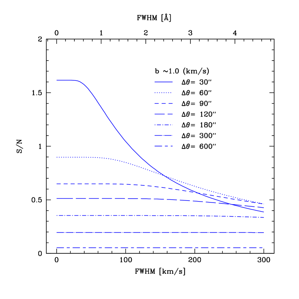
Figure 11: The expected signal to noise level (S/N) at which one can distinguish between an $\Omega_{m}=0.3,\Omega_{\Lambda}=0.7$ cosmology and a $\Omega_{m}=1.0$ cosmology from a single quasar pair as a function of resolution (FWHM). The effect of shot noise is included, with shot noise at the level of $b\sim 1.0$ km/s. We assume perfect knowledge of all of the other parameters involved in modeling the IGM.

In figure (11) we show the results of this calculation, in this case considering the difference between an $\Omega_{m}=1.0$ (EDS) cosmology and a $\Omega_{m}=0.3,\Omega_{\Lambda}=0.7$ (Lambda) cosmology. For a single pair with $\Delta\theta=30^{\prime\prime}$, at high observational resolution, one can already distinguish between the two models at $S/N\sim 1.6\sigma$. Still considering high observational resolution, we see that at larger separation, as the cross spectrum signal weakens, the S/N level goes down, reaching $S/N\sim 0.9\sigma$ at $\Delta\theta=60^{\prime\prime}$ and $S/N\sim 0.35\sigma$ at $\Delta\theta=180^{\prime\prime}$. At still larger separations, the discriminating power is quite weak, reaching $S/N\sim 0.2\sigma$ at $\Delta\theta=300^{\prime\prime}$ and $S/N<0.1$ at $\Delta\theta=600^{\prime\prime}$.

At lower observational resolution the advantage of measuring the cross spectrum for close separation pairs is lost. When the FWHM becomes slightly worse than $\sim 150$ km/s, the S/N level, at $S/N\sim 0.7\sigma$, is comparable for measuring the cross spectrum from a pair at separation $\Delta\theta=30^{\prime\prime}$ and for using a pair at separation $\Delta\theta=60^{\prime\prime}$. In order to obtain the increased discriminating power of small separation pairs, one must be able to resolve the high $k$ modes. At increased angular separation, however, observational resolution makes very little difference. At these separations the cross spectrum (see eq. 3) turns over at relatively low $k_{\parallel}$, and so, regardless of resolution, the high $k$ modes contribute insignificantly to the S/N level. This explains why the S/N curves at large angular separation in figure (11) are flat as a function of observational resolution. The conclusion is that there is an advantage to hunting out close separation pairs, but only if the observational resolution is sufficiently good. Below we give a rough formula to determine what spectral resolution is good for observing pairs of a given separation.

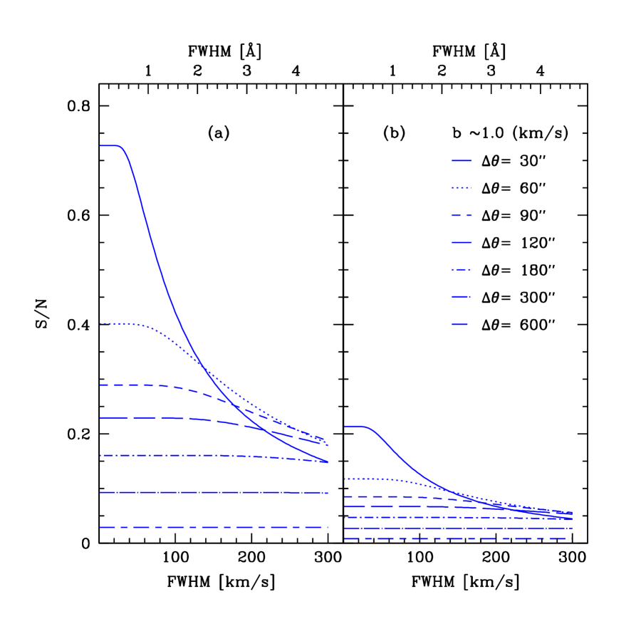
Figure 12: a) The same as figure (11) except this plot shows the S/N level at which one can distinguish between a $\Omega_{m}=0.3,\Omega_{\Lambda}=0.7$ cosmology and a $\Omega_{m}=0.2,\Omega_{\Lambda}=0.8$ cosmology from a single quasar pair. b) The S/N level at which one can distinguish between two quintessence cosmologies from a single quasar pair. Both cosmologies have $\Omega_{m}=0.3$ and $\Omega_{Q}=0.7$. The models have equations of state $w=-1$ and $w=-0.7$. The equation of state is assumed constant with redshift. In both a) and b), we assume perfect knowledge of all of the other parameters involved in modeling the IGM. It should be stressed that these comparisons are at $z\sim 3$. At sufficiently lower or higher redshifts, the AP test should have an increased sensitivity to $w$.

Figure (11) illustrates the possibilities of distinguishing between an EDS cosmology and a Lambda cosmology, but it is more interesting to consider the discriminating power between two more realistic cosmologies. In figure (12) we show the ability of the Ly$\alpha$ AP test to discriminate between a $\Omega_{m}=0.3,\Omega_{\Lambda}=0.7$ cosmology and a $\Omega_{m}=0.2,\Omega_{\Lambda}=0.8$ cosmology (left panel) as well as the ability to discriminate between two quintessence cosmologies (right panel). At high observational resolution, using a single pair with separation $\Delta\theta=30^{\prime\prime}$, one can expect to distinguish between the two Lambda cosmologies at a level of $S/N\sim 0.7$. With a pair at $\Delta\theta=60^{\prime\prime}$ the discriminating power falls off to $S/N\sim 0.4$ and then to $S/N\lesssim 0.2$ at $\Delta\theta=180^{\prime\prime}$ and $S/N\lesssim 0.1$ at $\Delta\theta=300^{\prime\prime}$. At the moderate resolution of ${\rm FWHM}\sim 150$ km/s, where the discriminating power is typically $S/N\sim 0.3$ for close separation pairs (with $\Delta\theta\sim 30-120^{\prime\prime}$), one needs $\sim 200$ pairs to distinguish between these models at the 4-$\sigma$ level. Alternatively, one could achieve the same discriminating power with only $\sim 35$ close separation ($\Delta\theta\sim 30^{\prime\prime}$), high resolution, pairs. We can provide a rough criterion for determining the spectral resolution that will be good for observing pairs at a given separation. We adopt the rule that the spectral resolution, FWHM, should be sufficiently good that the discriminating power drops off by no more than a factor of $0.7$ from its value at optimal resolution. Adopting this criterion for the case of discriminating between the two Lambda cosmologies, we find that the FWHM should be less than than $80(\Delta\theta/30^{\prime\prime})^{1.1}$ km/s for pairs with separations between $\Delta\theta=30^{\prime\prime}-100^{\prime\prime}$ and that the spectral resolution is pretty irrelevant for larger separation pairs. At separations between $\Delta\theta=30^{\prime\prime}-600^{\prime\prime}$, we find that the following fitting formula describes the expected discriminating power for a pair with a given separation and FWHM to better than $10\%$:

$$\frac{S}{N}(\theta,FWHM)\sim\frac{0.727\left(\frac{30^{\prime\prime}}{\theta}\right)^{0.83}-0.015\left(\frac{300^{\prime\prime}}{\theta}\right)^{-1.1}}{1-\left(0.7\ \frac{30^{\prime\prime}}{\theta}\frac{FWHM}{300km/s}\right)+\left(3.0\ \frac{30^{\prime\prime}}{\theta}\frac{FWHM}{300km/s}\right)^{2}-\left(1.6\ \frac{30^{\prime\prime}}{\theta}\frac{FWHM}{300km/s}\right)^{3}}$$ (9)

In the right hand panel of figure (11), we show the ability of the Ly$\alpha$ AP test to discriminate between a quintessence cosmology with equation of state $w=-1$ and a cosmology with $w=-0.7$. Here the pressure of the quintessence component is $p=w\rho_{Q}$, where $\rho_{Q}$ is the energy density of the quintessence component, and we assume that the equation of state is constant with redshift so that $\rho_{Q}=\Omega_{Q}(1+z)^{3(1+w)}$. As mentioned in §2, and illustrated in figure (1), the Ly$\alpha$ forest AP test is barely sensitive to $w$, at $z\sim 3$. We will be making a small error here in the predicted signal for $w=-0.7$, because the redshift distortions in this cosmology should be slightly different than in the $w=-1$ cosmology. We find that, indeed, even with high observational resolution, the discriminating power is only $S/N\sim 0.2$ for a single pair separated by $\Delta\theta=30^{\prime\prime}$. Discriminating between two quintessence models with the Ly$\alpha$ forest AP test would require an extremely large number of close separation pairs. The Ly$\alpha$ forest AP test may, however, be helpful for attempts to constrain quintessence models by helping to tighten constraints on $\Omega_{m}$, as mentioned in §2, and emphasized by McDonald (2003). Alternatively, applying the forest AP test to lower or higher redshifts might be a more promising way of constraining $w$ (see figure 1).

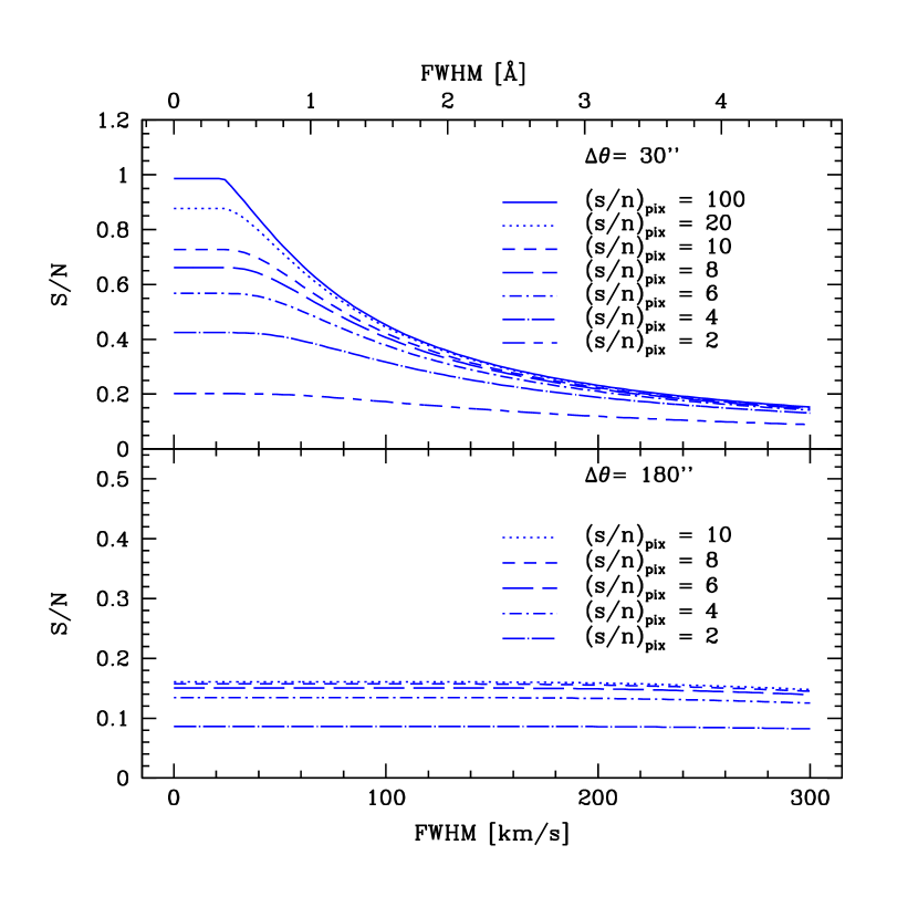
Figure 13: The plot shows the effects of shot noise on the S/N level at which one can distinguish between a flat $\Omega_{\Lambda}=0.7$ cosmology and a flat $\Omega_{\Lambda}=0.8$ cosmology. The top panel is for a single quasar pair separated by $\Delta\theta=30.0^{\prime\prime}$ and the bottom panel for $\Delta\theta=180.0^{\prime\prime}$. The different curves represent different assumptions about the typical signal to noise level per pixel, $(s/n)_{\rm pix}$ in each quasar spectrum. In each case the signal to noise level refers to the level at the continuum for a pixel size of $\Delta u=70$ km/s. The equivalent signal to noise level for a pixel of arbitrary size, $\Delta u$, is $(s/n)_{\rm pix}\times\left(\frac{\Delta u}{70km/s}\right)^{1/2}$. We assume perfect knowledge of all of the other parameters involved in modeling the IGM.

It is also instructive to consider the effect of shot-noise on our ability to discriminate between cosmologies. Since the noise fluctuations in each line of sight are independent, the noise has no cross-correlation and shot-noise does not directly contribute to our estimator for the cross spectrum. However, shot noise does contribute to the variance of our estimate for the cross spectrum. Here we estimate the shot noise level, at some typical signal to noise level per pixel, $(s/n)_{\rm pix}$, using an approximate formula from Hui et al (2001). If the typical signal to noise level per pixel at the continuum is $(s/n)_{\rm pix}$, the pixel separation $\Delta u$, and the mean transmission $\langle f\rangle$, then the shot-noise bias is $b\sim\frac{\Delta u}{\langle f\rangle}\left((s/n)_{\rm pix}\right)^{-2}$. For instance, in the above discussion we assumed $b\sim 1.0$ km/s, which for $\langle f\rangle=0.684$, $\Delta u=70$ km/s ($\sim 1\AA$ at $z\sim 2.82$), corresponds to a signal to noise per pixel of $(s/n)_{\rm pix}\sim 10$. In figure (13) we show the expected discriminating power (between Lambda cosmologies with $\Omega_{\Lambda}=0.7$ and $0.8$) for $(s/n)_{\rm pix}=2,4,6,8,10,20$ and $100$, with $\Delta u=70$ km/s, for a close separation pair separated by $\Delta\theta=30^{\prime\prime}$. We also show the discriminating power for a moderate separation pair, with $\Delta\theta=180^{\prime\prime}$, at shot noise levels corresponding to $(s/n)_{\rm pix}=2,4,6,8,10$. Given the plot we can ask how low a shot-noise level is required so that the expected discriminating power, from a pair with a given separation and spectral resolution, is degraded by no more than a factor of $0.7$ from its optimal value. We will take this as a criterion for determining what $(s/n)_{\rm pix}$ level is good for a pair at a given separation, observed with a given spectral resolution. For the pair separated by $\Delta\theta=30^{\prime\prime}$, at high spectral resolution, the discriminating power is degraded by a factor of $0.7$ when the signal to noise level reaches $(s/n)_{\rm pix}\sim 10$. At lower spectral resolution, FWHM $\sim 150$ km/s, the discriminating power is reduced by the same factor only when the signal to noise level reaches $(s/n)_{\rm pix}\sim 3-4$. For the pair separated by $\Delta\theta=180^{\prime\prime}$, the spectral resolution is unimportant and the discriminating power is degraded by a factor of $0.7$ when the signal to noise level reaches $(s/n)_{\rm pix}\sim 3-4$. In general shot-noise is an issue only when its contribution to the cross spectrum error becomes comparable to the sample variance contribution. The two contributions to the variance become comparable roughly when $b\sim P_{\rm 1d}(k)$; if $b\sim 1$ km/s, (corresponding to $(s/n)_{\rm pix}\sim 10$), the two are comparable near $k\sim 0.06$ s/km, at which scale the cross spectrum is very small unless the separation of the pair is also very small. With this level of shot-noise, the discriminating power will only be degraded for high-resolution, close separation pairs. If the shot-noise is sufficiently bad, however, the shot-noise contribution to the cross spectrum variance can become comparable to the sample variance contribution even on large scales. In this case, which occurs around $(s/n)_{\rm pix}\sim 3-4$, the shot-noise will degrade the discriminating power even for large separation pairs, as illustrated in the lower panel of figure (13). To summarize, for close separation pairs, with $\Delta\theta\sim 30^{\prime\prime}$, and high spectral resolution, given a pixel size of $\Delta u$, a signal to noise level of $(s/n)_{\rm pix}\sim 10\left(\frac{\Delta u}{70km/s}\right)^{1/2}$ is recommended. In other cases, $(s/n)_{\rm pix}\sim 4\left(\frac{\Delta u}{70km/s}\right)^{1/2}$ is generally adequate.

7 Conclusions

In this paper we have described a concrete procedure for obtaining constraints on dark energy from a version of the Ly$\alpha$ AP test. We applied this procedure to a small sample of quasar pairs, and discussed the possibilities of future observations. Our main results are summarized as follows:

• While the Ly$\alpha$ AP test is a sensitive discriminator of a cosmological constant, it is not sensitive to the equation of state of a quintessence field unless $w(z\sim 3)\gtrsim-0.4$. (See also McDonald 2003.) The Ly$\alpha$ AP test is particularly sensitive to the presence of a large $\Omega_{\Lambda}$.

• The effect of redshift distortions on the cross spectrum are important and must be taken into account in detail. At a redshift of $z=2.82$ we measure the quadrapole to monopole ratio of the flux power spectrum and find that a linear theory prediction is close to correct on large scales. The ratio depends somewhat on $\langle f\rangle$. The lesson is that one needs simulations to account for redshift distortions accurately.

• We measured the cross spectrum from a sample of close quasar pairs. The cross spectrum measurements have large error bars due to the small number of pairs in the present sample. The measurements are generally consistent with the cross spectra from a grid of simulated models, if perhaps weakly favoring high $\Omega_{\Lambda}$ cosmologies, although one pair, Q2139-4504A/B, has somewhat excess small scale power. A comparison between models from the simulation grid and the cross spectra of Q2139-4433/34 and the KP triplet disfavors an EDS cosmology at a level of $\sim 1.5\sigma$. If we include the poorly fit pair, an EDS cosmology is disfavored at $\gtrsim 2\sigma$. Future, more accurate measurements of the cross spectra will require comparison with a larger grid of simulated models.

• We consider the expected power of future observations to discriminate between different cosmological geometries. A sample of $\sim 50$ moderate resolution, FWHM $\sim 150$ km/s, close separation pairs (with $\Delta\theta\sim 30^{\prime\prime}-120^{\prime\prime}$) should be able to discriminate between an $\Omega_{\Lambda}=0.7$ and an $\Omega_{\Lambda}=0.8$ cosmology at the $\sim 2\sigma$ level, ignoring degeneracies with other IGM modeling parameters. We find that there is a sizeable advantage obtained by observing very close, $\Delta\theta\sim 30^{\prime\prime}$, separation pairs with high spectral resolution, provided simulation measurements are reliable at high $k$. Given $\sim 10$ high resolution, $\Delta\theta\sim 30^{\prime\prime}$ separation pairs, we should be able to distinguish between the two Lambda cosmologies at the $2\sigma$ level.

  One should be able to obtain this type of sample with quasar pairs discovered by the Two Degree Field (2df) and SDSS surveys, provided one does some follow-up spectroscopy (Burles, private communication 2003). Two remarks may be helpful in this regard. First, due to the finite optical fiber size, SDSS selects against quasar pairs with separation less than 55”. One can attempt to recover pairs with these separations by looking for objects with similar colors nearby existing quasars. Second, SDSS has a spectroscopic cut-off at 3800 Å. One can recover many more pair spectra by going down to a lower cut-off of $\sim 3400$ Å. Since the auto spectrum has not yet been measured at the low redshifts corresponding to these wavelengths, one would also need to use the spectra in the sample to measure the auto spectrum at $z\sim 1.8$.

Finally, we mention a few words about future work. As the error bars on cross spectrum measurements get smaller in the future, it will be important to use higher resolution, larger volume simulations. It will also be important to test the accuracy of our N-body plus smoothing technique against full hydrodynamic simulations, especially if we aim to compare data and theory at high $k$ where the hydrodynamic effects should be most important. Measurements of the cross spectrum may also be useful in other pursuits such as recovering the linear mass power spectrum (Viel et al. 2002), reconstructing a three dimensional map of the density field in the IGM (Pichon et al. 2001), and constraining the effect of feedback on the IGM found by Adelbeger et al. (2003).

AL and LH are supported in part by the Outstanding Junior Investigator Award from the DOE, AST-0098437 grant from the NSF, and by National Computational Science Alliance under grant AST030027, utilizing the Origin 2000 array. AC acknowledges support from grant AST-0098258 from the NSF and AR-9195 from STScI. MZ was supported by the David and Lucille Packard Foundation and the NSF. AL thanks the Fermilab theoretical astrophysics department for hospitality. We thank Nick Gendin for the use of his PM code, Roman Scoccimarro for discussions and for reading a draft, and Scott Burles for discussions about the expected number of quasar pairs from 2df and SDSS.

Appendix A

In this section we mention some details regarding the simulations that we run and show some convergence tests with respect to resolution and box size.

All of our simulations are run in an SCDM cosmology with the same linear transfer function. We use the Ma (1996) transfer function, which is a modified version of the BBKS transfer function (Bardeen et al. 1996). We assume a shape parameter of $\Gamma=\Omega_{m}h=0.5$, and a normalization of $\sigma_{8}(z=0)=0.82$. We run all simulations assuming an $\Omega_{m}=1$ cosmology so that the linear growth factor is just proportional to $1+z$. In this case it is easy to use different simulation outputs to represent different power spectrum normalizations. The box units are converted into units of km/s assuming the EDS cosmology. Although this is a rather disfavored shape for the initial linear power spectrum, our purpose here is to span a range of power spectrum shapes and amplitudes near $z\sim 3$ in units of km/s, at scales around $1$ h/Mpc, for which this initial power spectrum template is adequate. In a different cosmology the conversion between units of comoving $Mpc/h$ and observed $km/s$ units will require different initial linear power spectra to fit the observed flux auto spectra; however the differing initial power spectra must all lead to similar flux power spectra in units of $km/s$ at $z\sim 3$. We do, however, then neglect the dependence of dynamics and redshift distortions on $\Omega_{m}$. For flat models with a cosmological constant, we should only be making a small error since $\Omega_{m}(z\sim 3)\sim 1$. (For tests see Croft et al. 1998, Gnedin & Hamilton 2002). We examine a range of different power spectrum amplitudes and slopes. To investigate a range of power spectrum normalizations, we save the density and velocity fields from the simulations at a range of output times. Different power spectrum shapes are examined by considering a range of primordial spectral indices.

Simulations of the Ly$\alpha$ forest are challenging in that the requirements on box size and resolution are fairly stringent. On the smallest scales, one must resolve the pressure smoothing scale, which is typically $k_{f}\sim 35$ h Mpc^-1 for an SCDM cosmology. One also needs to resolve the thermal broadening scale which smooths the optical depth on scales of $k_{\rm th}\sim 0.1$ s/km, for $T_{0}=10^{4}$ K. On the largest scales one requires a boxsize large enough that fluctuations on the box scale are still in the linear regime, and such that the box has a sufficient volume to provide a representative sample of the universe. In figure (14) we show a test of the resolution of our simulation box. In this figure we show the flux auto and cross spectra from two simulations run in the same model, each with a box size of $20.0$ Mpc/h, but one with $256^{3}$ particles and the other with $512^{3}$ particles. Right at the fundamental mode, probably due to the small number of modes available in the simulation box, the auto and cross spectra from the $512^{3}$ simulation are substantially larger than those from the $256^{3}$ simulation, otherwise the spectra from the low and high resolution simulations are consistent on large scales. In comparing the observed auto spectrum with simulation models we thus neglect scales with $k<2\times k_{\rm fun}$, where $k_{\rm fun}$ is the fundamental mode of the simulation box. In comparing the cross spectrum with simulation models we include these modes, which should be adequate since the error bars on the cross spectrum are very large on such scales. On small scales the $256^{3}$ simulation clearly misses small scale flux power in the auto spectrum, primarily at $k\gtrsim 0.03$ s/km. Since we rely in this paper on $256^{3}$ simulations, we then only include data with $k\lesssim 0.03$ s/km in comparing our models with observations, as mentioned in §3.1. The cross spectrum, at separation $\Delta\theta=33^{\prime\prime}$, on the other hand, is actually slightly larger on small scales in the $256^{3}$ simulation than in the $512^{3}$ simulation. In this paper, our data have poor resolution, (see Table 1 and the dotted lines in the figure), so we do not use the high $k$ simulation points in comparing with data anyway. In figure (15) we show a box size test. The figure shows a comparison between cross and auto spectra measured in a $128^{3}$ particle, $20.0$ Mpc/h box size simulation and those measured in a $256^{3}$ particle, $40.0$ Mpc/h box size simulation. The two simulations thus have the same resolution, but one has twice the box size of the other. Additionally we show the auto and cross spectra in the smaller volume simulation using the same model, but averaged over 5 different realizations of the simulation box. On small scales the auto and cross spectra are quite similar. On large scales one can see the sample variance error from having only one realization of the smaller box. The figure also shows that this error is quite reduced by averaging over 5 different simulation realizations of the smaller volume box. In conclusion, it is less than ideal to obtain constraints from a single realization of a $256^{3}$, $20.0$ Mpc/h simulation box. Especially as the error bars on the observed auto and cross spectra decrease, it will be necessary to simulate a larger volume at higher resolution.

Table 1: Pairs for Cross-Correlation Analysis

QSO Pair	$z_{1}$, $z_{2}$	$\lambda_{\rm low}$(Å) - $\lambda_{\rm high}$(Å)	$\bar{z}_{Ly\alpha}$	$\Delta\theta$ (arcsec)
Q2139-4504A/B	3.06, 3.25	4467.56 – 4811.62	2.82	33
Q2139-4433/34	3.22, 3.23	4456.54 – 5000.52	2.89	62
KP76/77	2.467, 2.521	3809.60 – 4108.31	2.26	147
KP76/78	2.467, 2.607	3809.60 – 4108.31	2.26	130
KP77/78	2.521, 2.607	3809.60 – 4108.31	2.26	180

Note. — A summary of the quasar pairs included in the cross-correlation analysis. The first column gives the names of the members of the QSO pair, the second column gives the redshifts of each member of the pair, the third column shows the wavelength range analyzed, the fourth column indicates the mean redshift of absorption in the Ly$\alpha$ forest, and the fifth column is the separation of the pair in arcseconds. The pair Q2139-4433/34 has a typical resolution of FWHM = $3.6$ Å, the pair Q2139-4504A/B has a typical resolution of FWHM = $3.0$ Å, and the KP triplet has a typical resolution of FWHM = $2.79$ Å.

Figure 14: A resolution test, showing the flux auto and cross spectra for a $256^{3}$ particle, $20.0$ Mpc/h boxsize simulation and those measured from a $512^{3}$ particle, $20.0$ Mpc/h simulation in the same model. The assumed IGM model is $(a,n,k_{f},T_{0},\alpha,\langle f\rangle)=(0.19,0.7,35.0$ h Mpc^-1, $250$ (km/s)², $0.2,0.684)$. The cross spectrum is computed assuming $\Omega_{m}=0.3$. The comparison is shown for a single simulation realization at each resolution. The dotted curves show the cross spectra convolved with the instrumental resolution of the close separation pairs studied in §5.

Figure 15: A boxsize test, showing the flux auto and cross spectra for a $128^{3}$ particle, $20.0$ Mpc/h boxsize simulation and those measured from a $256^{3}$ particle, $40.0$ Mpc/h simulation in the same model. The assumed IGM model is $(a,n,k_{f},T_{0},\alpha,\langle f\rangle)=(0.19,0.7,35.0$ h Mpc^-1, $250$ (km/s)², $0.2,0.684)$. The cross spectrum is computed assuming $\Omega_{m}=1.0$, and shown at separations of $\Delta\theta=33^{\prime\prime}$ and $\Delta\theta=60^{\prime\prime}$. The auto spectrum shown here comes from the average of $6,000$ lines of sight taken along each of the simulation box axes. The cross spectra come from the average of $3,000$ pairs of lines of sight along each of the simulation box axes. The black dotted lines shows the result of averaging measurements of the auto and cross spectrum over 5 independent simulation realizations of the same model using the small volume simulations.

References

- (1) Adelberger, K. L. A., Steidel, C. C., Shapley, A. E., & Pettini, M. 2003, ApJ, 584, 45
- (2) Alcock, C. & Paczynski. B. 1979, Nature, 281, 358
- (3) Ballinger, W. E., Peacock, J. A., & Heavens, A. F. 1997, MNRAS, 282, 877
- (4) Bajtlik, S., Duncan, R. C., & Ostriker, J. P. 1988, ApJ, 327, 570
- (5) Bardeen, J. M., Bond, J. R., Kaiser, N., & Szalay, A. S. 1986, ApJ, 304, 15
- (6) Bechtold, J., Crotts, A. P. S., Duncan, R. C., & Fang, Y. 1994, ApJ, 437, L83
- (7) Bernardi, M. et al. 2002, ApJ submitted, (astro-ph 0206293)
- Bi & Davidsen (1997) Bi, H. & Davidsen, A. F., 1997, ApJ 479, 523
- Bond & Wadsley (1997) Bond, J. R. & Wadsley, J. W., 1997, Proc. 12th Kingston Conf., Halifax, (astro-ph 9703125)
- Bryan et al. (1999) Bryan, G., Machacek, M., Anninos, P., & Norman, M. L. 1999, ApJ, 517, 13
- (11) Cen, R., Miralda-Escudé, J., Ostriker, J. P., Rauch, M. 1994, ApJ, 437, L9
- (12) Cole, S., Fisher, K. B., & Weinberg, D. 1994, MNRAS, 267, 785
- Croft et al. (1998) Croft, R. A. C., Weinberg, D. H., Katz, N., & Hernquist, L., 1998a, ApJ 495, 44
- (14) Croft, R. A. C., Weinberg, D. H., Pettini, M., Hernquist, L., & Katz, N. 1999, ApJ, 520, 1
- Croftet al. (2002) Croft, R. A. C., Weinberg, D. H., Bolte, M., Burles, S., Hernquist, L., Katz, N., Kirkman, D., & Tytler, D. 2002, ApJ, 581, 20
- (16) Crotts, A. P. S., & Bechtold, J. 2003, (in preparation)
- (17) Crotts, A. P. S., & Fang, Y. 1998, ApJ, 502, 16
- (18) Fry, J. N. 1994, PRL, 73, 215
- (19) Gaztanaga, E., & Croft, R. A. C. 1999, MNRAS, 309, 885
- (20) Gnedin, N. Y, & Hui, L. 1998, MNRAS, 296, 44
- (21) Gnedin, N. Y, & Hamilton, A. J. S., 2002, MNRAS, 334, 107
- (22) Gunn, J. E., & Peterson, B. A. 1965, ApJ, 142, 1633
- (23) Hamilton, A. J. S., & Tegmark, M. 2002, MNRAS, 330, 506
- (24) Hatton, S., & Cole, S. 1998, ApJ, 296, 10
- Hernquist et al. (1996) Hernquist, L., Katz, N., Weinberg, D. H., & Miralda-Escudé, J., 1996, ApJ 457, L51
- (26) Hoyle, F., Outram, P. J., Shanks, T., Boyle, B. J., Croom, S. M., Smith, R. J. 2002, MNRAS, 332, 311
- Hui, Gnedin & Zhang (1997) Hui, L., Gnedin, N. Y., & Zhang, Y., 1997, ApJ 486, 599
- Hui & Gnedin (1997) Hui, L. & Gnedin, N. Y., 1997, MNRAS 292, 27
- (29) Hui, L., Stebbins, A., & Burles, S. 1999, ApJ, 511, L5
- (30) Hui, L. 1999, ApJ, 516, 519
- (31) Hui, L., Burles, S., Seljak, U., Rutledge, R. E., Magnier, E., & Tytler, D. 2001, ApJ, 552, 15
- (32) Kaiser, N. 1987, MNRAS, 227, 1
- (33) Kaiser, N. & Peacock, J. A. 1991, ApJ, 379, 482
- (34) Kujat, J., Linn, A. M., Scherrer, R. J., & Weinberg, D. H. 2002, ApJ, 572, 1
- (35) Lin, W. & Norman, M. L., 2002, (astro-ph 0211177)
- (36) Ma, C.-P., 1996, ApJ, 471, 13
- (37) Matsubara, T. & Suto, Y. 1996, ApJ, 470, L1
- (38) Matsubara, T. & Szalay, A. 2002, PRL, submitted (astro-ph 0208087)
- (39) McDonald, P. & Miralda-Escudé, J. 1999, ApJ, 519, 486
- (40) McDonald, P., Miralda-Escudé, J., Rauch, M., Sargent, W. L. W., Barlow, T. A., Cen, R., & Ostriker, J. P., 2000a, ApJ, 543, 1
- (41) McDonald, P. 2003, ApJ, 585, 34
- (42) Meiksin, A. & White, M., 2001, MNRAS, 2001, 324, 141
- (43) Meiksin, A., & White, M., 2003, submitted to MNRAS, astro-ph 0307289
- Muecket et al. (1996) Muecket, J. P., Petitjean, P., Kates, R. E., & Riediger, R., 1996, A&A 308, 17
- (45) Nusser, A., Haehnelt, M. 1999, MNRAS, 303, 179
- (46) Outram, P. J., Hoyle, F., Shanks, T., Boyle, B. J., Croom, S. M., Loaring, N. S., Miller, L., & Smith, R. J., 2001, MNRAS, 328, 1740
- (47) Perlmutter, et al. 1999, ApJ, 517, 565
- (48) Phillips, S. 1994, MNRAS, 269, 1077
- (49) Pichon, C., Vergely, J. L., Rollinde, E., Colombi, S., & Petitjean, P. 2001, MNRAS, 326, 597
- (50) Popowski, P. A., Weinberg, D. H., Ryden, B. S., & Osmer, P. S. 1998, ApJ, 498, 11
- (51) Press, W. H., Rybicki, G. B., & Schneider, D. P. 1993, ApJ, 414, 64
- (52) Rauch, M. et al. 1997, ApJ, 489, 7
- (53) Rauch, M., Sargent, W. L., Barlow, T. A., Carswell, R. F. 2001, ApJ, 562, 76
- (54) Riess, A. et al. 1998, AJ, 116, 1009
- (55) Rollinde, E., Petitjean, P., Pichon, C., Colombi, S., Aracil, B., D’Odorico, V., & Haehnelt, M. G., 2003, MNRAS, submitted (astro-ph 0302145)
- (56) Ryden, B. S. 1995, ApJ, 452, 25
- (57) Ryden, B. S., & Melott, A. L., 1996, ApJ, 470, 160
- (58) Scoccimarro, R., Couchman, H. M. P., & Frieman, J. A., 1999, ApJ, 517, 531
- (59) Scoccimarro, R., Feldman, H. A., Fry, J. N., Frieman, J. A. 2001, ApJ, 546, 652
- (60) Scoccimarro, R. & Sheth, R. 2002, MNRAS, 329, 629
- (61) Seljak, U., McDonald, P., & Makarov, A. 2003, submitted to MNRAS, astro-ph 0302571
- (62) Seo, H.-J., Eisenstein, D. J. 2003, submitted to ApJ, astro-ph 0307460
- (63) Spergel, D. et al. 2003, ApJ, in press, astro-ph 0302209
- (64) Tegmark, M. & Zaldarriaga, M. 2000, ApJ, 544, 30
- Theuns et al. (1999) Theuns, T., Leonard, A., Schaye, J., & Efstathiou, G. 1999, MNRAS, 303L, 58
- (66) Theuns, T. et al. 2002, ApJ, 574, L111
- (67) Verde, L. et al. 2002, MNRAS, 335, 432
- (68) Viel, M., Matarrese, S., Mo, H. J., Haehnelt, M. G., Theuns, T., 2002, MNRAS 329, 848
- (69) Viel, M., Matarrese, S., Heavens, A., Haehnelt, M. G., Kim, T. S., Springel, V., & Hernquist, L. 2003, submitted to MNRAS, astro-ph 0308151
- (70) Zaldarriaga, M., Hui, L., & Tegmark, M., 2001a, ApJ, 557, 519
- (71) Zaldarriaga, M., Seljak, U., & Hui, L., 2001b, ApJ, 551, 48
- (72) Zaldarriaga, M., 2002, ApJ, 564, 153
- (73) Zaldarriaga, M., Scoccimarro, R., & Hui, L., 2003, ApJ, 590, 1
- (74) Zehavi, I. et al. 2003, submitted to ApJ, astro-ph 0301280
- (75) Zhang, Y., Anninos, P., & Norman, M. L., 1995, ApJL, 453, L57