Formation of Dwarf Galaxies during the Cosmic Reionization

Abstract

We reanalyze the photoevaporation problem of subgalactic objects irradiated by ultraviolet background (UVB) radiation in a reionized universe. For the purpose, we perform three-dimensional radiation smoothed-particle-hydrodynamics (RSPH) calculations, where the radiative transfer is solved by a direct method and also the non-equilibrium chemistry of primordial gas including H₂ molecules is incorporated. Attention is concentrated on radiative transfer effects against UVB for the formation of subgalactic objects with $T_{\rm vir}\lesssim 10^{4}$K. We consider the reionization model with $z_{\rm reion}\approx 7$ and also the earlier reionization model ($z_{\rm reion}\approx 17$) inferred by the WMAP. We find that the star formation is suppressed appreciably by UVB, but baryons at high-density peaks are self-shielded even during the reionization, forming some amount of stars eventually. In that sense, the photoevaporation for subgalactic systems is not so perfect as argued by one-dimensional spherical calculations. The final stellar fraction depends on the collapse epoch and the mass of system, but almost regardless of the reionization epoch. For instance, a few tenths of formed stars are born after the cosmic reionization in $z_{\rm reion}\approx 7$ model, while more than 90% stars are born after the reionization in the WMAP reionization model. Thus, effects of UVB feedback on the substructure problem with a cold dark matter (CDM) scenario should be evaluated with careful treatment of the radiative transfer.

The star clusters formed at high-density peaks coalesce with each other in a dissipationless fashion in a dark matter potential, resultantly forming a spheroidal system. As a result, these low-mass galaxies have large mass-to-light ratios such as observed in dwarf spheroidals (dSph’s) in the Local Group.

1 Introduction

In the context of cold dark matter (CDM) cosmology, the first generation of objects should have the mass of $\sim 10^{6}M_{\odot}$ and form at redshifts of $20\lesssim z\lesssim 50$ (Tegmark et al., 1997; Fuller & Couchman, 2000). At later epochs, the first objects are assembled into larger systems in a hierarchical fashion to form dwarf or normal galaxies. On the other hand, it is thought that the universe was reionized at $z>5$, because the absorption by the neutral intergalactic medium (IGM) is observed to be feeble at redshifts $z\lesssim 4$. The reionization redshift is inferred to be $z_{\rm reion}\approx 6$ from the spectra of high-$z$ quasars (Djorgovski et al. 2001, and references therein), $6\lesssim z_{\rm reion}\lesssim 10$ from simulations on Ly$\alpha$ absorption lines (Umemura, Nakamoto, & Susa, 2001), or $11\lesssim z_{\rm reion}\lesssim 30$ from the recent results of WMAP (Kogut et al., 2003). Thus, it is anticipated that the UVB directly influences the assembly phase of galaxies. The UVB has several important physical impacts on the galaxy formation. One of the most important effects is the photoheating. If a gas cloud is irradiated by UVB, the gas temperature is raised up to $T\sim 10^{4}-10^{5}$K, so that gaseous systems with virial temperature of $T\lesssim 10^{4}$ K can be evaporated owing to the enhanced thermal pressure (Umemura & Ikeuchi, 1984; Dekel & Rees, 1987; Efstathiou, 1992; Babul & Rees, 1992; Thoul & Weinberg, 1996; Ferrara & Tolstoy, 2000; Gnedin, 2000c; Shapiro & Raga, 2001; Shaviv & Dekel, 2003). Such an effect by UVB may reconcile the paradox that low mass galaxies are overproduced in CDM cosmology, compared with observations (White & Frenk, 1991; Kauffmann, White, & Guiderdoni, 1993; Cole et al., 1994; Moore et al., 1999; Binney, Gerhard, & Silk, 2001). The criterion for photoevaporation has been derived from detailed hydrodynamic calculations by Umemura & Ikeuchi (1984) and Thoul & Weinberg (1996). However, if the systems are self-shielded against the UVB, the criterion for photoevaporation is completely changed. The self-shielding comes from the radiative transfer effects of ionizing photons. Tajiri & Umemura (1998) have derived the self-shielding criterion by solving full radiative transfer for spherical clouds, to find the critical optical depth of 2.4. Also, if the system is self-shielded from UVB, the gas can cool below $10^{4}$ K by H₂ cooling (Susa & Kitayama, 2000). The complete radiation-hydrodynamic calculations have been done for spherical clouds by Kitayama et al. (2001), where hydrodynamics, radiative transfer, and primordial gas chemistry including H₂ molecules are self-consistently incorporated, and thereby the criteria for cloud collapse have been derived depending on the redshifts. Very recently, pioneering approaches with three-dimensional hydrodynamics have started on this isuue in the context of CDM cosmology. They are, for example, the simulations by Ricotti, Gnedin, & Shull (2002a, b) with radiative transfer based on the optically thin variable Eddington tensor (OTVET) approximation, and by Tassis et al. (2003) with optically-thin approximation.

If the nonlinear evolution of density fluctuations proceed in a hierarchical fashion, two major effects by radiative transfer are expected. One is the direct effect, that is, the self-shielding of density peaks that collapse prior to the reionization (Gnedin, 2000c; Nakamoto, Umemura, & Susa, 2001; Razoumov et al., 2002; Ricotti, Gnedin, & Shull, 2002a, b). The other is the enhancement of H₂ formation in relatively massive fluctuations which are once ionized and then self-shielded in the course of mass accretion. The second effect has been pointed out by many authors so far (Kang & Shapiro, 1992; Corbelli, Galli & Palla, 1997; Susa & Umemura, 2000). These two effects play a substantial role for the galaxy formation under UVB, especially if the star formation process is taken into account in collapsing clouds, because star formation activities in galaxies appear to be strongly correlated to cold HI gas with a few $\times 10^{3}$K (Young & Lo, 1997a, b). Therefore, the effects of radiation transfer of ionizing photons should be carefully treated to elucidate the galaxy formation process under UVB. In this paper, we perform 3D SPH calculations, incorporating radiation transfer and primordial gas chemistry. Here, we focus on relatively low mass galaxies, where the dynamics is likely to be strongly subject to UVB. The evolution of subgalactic systems is significant also for the formation of massive galaxies, since the self-shielding against UVB can be responsible to overall SFH in the galaxies and therefore resultant galactic morphology (Susa & Umemura, 2000).

The goal of this paper is to elucidate how the photoevaporation of subgalactic systems is caused by UVB and how the star formation history (SFH) is influenced consequently. The paper is organized as follows. In §2, the numerical methods are described. In §3, the results of simulations are presented. In §4, the SFH is discussed in relation to the inferred SFH in dwarf galaxies. §5 is devoted to the conclusions.

2 Numerical Methods

We have performed numerical simulations on the single halo collapse with SPH particles ($2^{15}$) and dark matter particles ($2^{15}$). The halo mass ranges from $M_{\rm halo}\approx 6\times 10^{7}$ to $6\times 10^{8}M_{\odot}$. The initial conditions are set by COSMICS. The radiative transfer of the UV radiation field is solved assuming a single source outside the simulation box, coupled with the detailed chemistry of primordial gas. We also have taken into account the numerical “star formation”. Following subsections are devoted to describe some details of the scheme.

2.1 Hydrodynamics and Gravity

Hydrodynamics is calculated by Smoothed Particle Hydrodynamics (SPH) method. We use the version of SPH by Umemura (1993) with the modification according to Steinmetz & Müller (1993), and also we adopt the particle resizing formalism by Thacker et al. (2000). The gravitional force is calculated by a special purpose processor for gravity calculation, GRAPE (Sugimoto et al., 1990), which can also accelerate an SPH scheme (Umemura et al., 1993). Here, we used the latest version, GRAPE-6 (Makino, 2002), which has the speed of 1Tflops. Eight GRAPE-6 boards are combined with CP-PACS, which is a massively parallel supercomputer in University of Tsukuba, composed of 2,048 processing units, with theoretical peak speed of 614 Gflops (Iwasaki, 1988). This system is called the Heterogeneous Multi-Computer System (HMCS) (Boku et al., 2002). The hydrodynamics, radiative transfer, and chemical reactions are solved with CP-PACS. The originally developed software for HMCS can be easily applied to any massively parallel computer connected through TCP-IP with GRAPE-6 boards. Actually, we also used an alpha-cluster and a PC-cluster instead of CP-PACS as the host.

The softening length for gravity is taken as $60$pc for all SPH and CDM particles. Also, the minimal size of SPH particle is introduced so as to prevent the simulation from stopping owing to very short local timescales. We have tested this scheme by the standard Sod’s shock tube and Evrard’s collapse problems, and the results well reproduce the known solutions.

2.2 Thermal Processes

The non-equilibrium chemistry and radiative cooling for primordial gas are calculated by the code developed by Susa & Kitayama (2000), in which H₂ cooling and reaction rates are taken from Galli & Palla (1998). The H₂ cooling rate induced by the collision with H atoms is plotted in Figure 1 for high ($10^{6}{\rm cm}^{-3}$) and low density ($0.1\,{\rm cm}^{-3}$) cases. The cooling functions by Hollenbach & McKee (1979) and Lepp & Shull (1983) are also plotted for reference. They agree with each other at the high density limit (i.e. LTE), whereas they disagree significantly with each other at the low density limit. We also assessed the contribution of metallic cooling, and compared it to H₂ and Ly$\alpha$ cooling in Figure 2 for the temperature below $10^{4}$K. The cooling rate by metals is evaluated by the fitting formula in Dalgarno & McCray (1972), assuming that the relative abundance between the heavy elements is the same as the solar neighbourhood. The fractions of electrons and H₂ are assumed to be the values behind a shock with the velocity of $v_{\rm s}>30{\rm kms^{-1}}$, since the initially ionized gas traces a similar path as the gas behind such a shock (Kang & Shapiro, 1992; Corbelli, Galli & Palla, 1997; Susa & Umemura, 2000). We also plot H₂ cooling function assuming the H₂ fraction of $10^{-4}$, which is favored for the clouds with virial temperature of $10^{3}{\rm K}\lesssim T_{\rm vir}\lesssim 10^{4}{\rm K}$(Nishi & Susa, 1999). As shown in Fig.2, for $T\lesssim 8\times 10^{3}$ K, the dominant cooling mechanism is dependent on the metallicity.

In nearby dwarf galaxies, the metal cooling is likely to be important, because the observed metallicity is $Z/Z_{\odot}\sim 10^{-2}-10^{-1}$. On the other hand, the observations of Ly$\alpha$ absorption systems at high redshifts imply that the metallicity of high-$z$ intergalactic medium (IGM) is at a level of $Z/Z_{\odot}\sim 10^{-2}-10^{-3}$ (Songaila, 2001). Hence, the cooling rate by metals is rather smaller than that by H₂, as long as $10^{3}{\rm K}\lesssim T\lesssim 10^{4}{\rm K}$. In the present paper, we focus on the primary star-forming phase in dwarf galaxies from metal poor gas with the metallicity seen in IGM or more primordial gas. If one pursues the subsequent recycling phase of interstellar medium with SN explosions, it is definitely requisite to include the metal cooling. Such a recycling effect is important for the chemical evolution of galaxies, but the issue is beyond the scope of present paper and left in future study.

It should be also noted that the effects by metals can play a significant role even at a level of $Z/Z_{\odot}\sim 10^{-5}$ for the runaway collapse onto a primordial protostar (Omukai, 2000; Bromm et al., 2001; Schneider et al., 2002), although here we do not pursue the runaway to a star in such dense, cold regions. Based upon these arguments, we neglect the cooling by metals in this paper, and the thermal processes are calculated with the chemistry for primordial abundance gas.

2.3 Radiative Transfer

The photoionization rate and the photoheating rate are respectively given by

$$k_{\rm ion} = n_{\rm HI}\int_{\nu_{L}}^{\infty}\int\frac{I_{\nu}\left(s\right)}{h\nu}\sigma_{\nu}d\Omega d\nu,$$ (1)

$$\Gamma_{\rm ion} = n_{\rm HI}\int_{\nu_{L}}^{\infty}\int\frac{I_{\nu}\left(s\right)}{h\nu}\sigma_{\nu}(h\nu-h\nu_{L})d\Omega d\nu.$$ (2)

Here $n_{\rm HI}$ represents the number density of neutral hydrogen, $\sigma_{\nu}$ is the photoionization cross section, $\nu_{\rm L}$ is the frequency at the Lyman limit, and $\Omega$ is the solid angle. $I_{\rm\nu}(s)$ is the intensity of the UV radiation with $s$ denoting the distance from the source of ionizing photons. $I_{\rm\nu}(s)$ is determined by solving radiative transfer equation:

$$\frac{dI_{\nu}}{ds} = -n_{\rm HI}\sigma_{\nu}I_{\nu},$$ (3)

where the reemission term is not included, because we employ on-the-spot approximation. The transfer equation (3) is solved based upon the method developed by Kessel-Deynet & Burkert (2000), which utilizes the neighbor lists of SPH particles to assess the optical depth from a certain source to an SPH particle. Here, we assume a single point source located very far from the simulated region, and control the UV intensity by specifying the incident flux to the simulation box as described in section 2.5. It is noted that the irradiation from one side can overestimate the effects of shadowing, and also internal sources, if they form, might play a significant role (Ricotti, Gnedin, & Shull, 2002a, b). On the other hand, in Kessel-Deynet & Burkert’s method, the numerical diffusion of radiation is not negligible. This effect tends to reduce the shadowing effect. These points should be improved in the future.

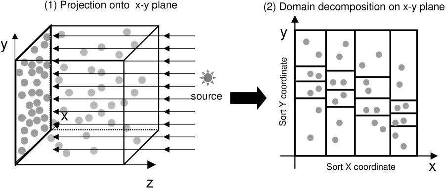
Figure 3: Parallelization of the code is schematically shown. (1) Particles are projected onto the $x-y$ plane which is perpendicular to the light ray. (2) The particles are sorted by $x-$ and $y-$ coordinates and decomposed into subclasses which include an equal number of particles. (3) Each subclass is assigned to each PU.

We parallelize the scheme so that we can implement it on massively parallel computer systems such as CP-PACS. For the purpose, particles should be classified into the subsets which are assigned to PUs. The domain decomposition is performed as shown in Figure 3. The first step is to project the particle positions onto the plane which is perpendicular to the light rays of the external single source. Since the position of source is assumed to be far away from the simulated region, we can approximate the light rays to be parallel. The second step is to sort the projected positions of particles on the $x-y$ plane. Then, with the results of coordinate sorting, we generate subsets with an equal number of particles, which are respectively assigned to computational domains, i.e. PUs. In Appendix, the test calculation using this scheme is presented for the propagation of ionization front in a uniform media. We remark that the present parallelization scheme is not valid for the multiple sources, because the domain decomposition is based upon the projection of all particles onto the plane perpendicular to the source direction. Hence, it is necessary to invoke a new technique in order to include internal sources in the future analysis.

Combining equations (1),(2) and (3), we can rewrite the ionization rate and the photoheating rate as follows:

$$k_{\rm ion} = -\frac{d}{ds}\int_{\nu_{L}}^{\infty}\int\frac{I_{\nu}\left(s\right)}{h\nu}d\Omega d\nu$$ (4)

$$= -\frac{d}{ds}\int_{\nu_{L}}^{\infty}\frac{F_{\nu}\left(s\right)}{h\nu}d\nu,$$

$$\Gamma_{\rm ion} = -\frac{d}{ds}\int_{\nu_{L}}^{\infty}\int\frac{I_{\nu}\left(s\right)}{h\nu}(h\nu-h\nu_{L})d\Omega d\nu$$ (5)

$$= -\frac{d}{ds}\int_{\nu_{L}}^{\infty}\frac{F_{\nu}\left(s\right)}{h\nu}(h\nu-h\nu_{L})d\nu.$$

When we need to assess the rates at each grid point (or each SPH particle), we use the following formula:

$$k_{\rm ion}\left(i+1/2\right) = \frac{1}{s_{i+1}-s_{i}}\left(\Phi_{1}(i)-\Phi_{1}(i+1)\right),$$ (6)

$$\Gamma_{\rm ion}\left(i+1/2\right) = \frac{1}{s_{i+1}-s_{i}}\left(\Phi_{2}(i)-\Phi_{2}(i+1)\right),$$ (7)

where

$$\Phi_{1}(s) = \int_{\nu_{L}}^{\infty}\frac{F_{\nu}\left(s\right)}{h\nu}d\nu,$$ (9)

$$\Phi_{2}(s) = \int_{\nu_{L}}^{\infty}\frac{F_{\nu}\left(s\right)}{h\nu}(h\nu-h\nu_{L})d\nu.$$ (10)

Here $i+1/2$ denotes the grid point at which the rates are assessed, and $i$ denotes the boundary between $i-1/2$ and $i+1/2$ grids. In the present simulation, these grids are generated by the method in Kessel-Deynet & Burkert (2000). The above formula has an important advantage that the propagation of ionization front is properly traced even for a large grid size with optical depth greater than unity ($\tau>1$) (Kessel-Deynet & Burkert, 2000; Abel, Norman & Madau, 1999).

2.4 Star Formation Algorithm

Here the “star formation” algorithm used in this simulation is described. At each time step, we pick up the SPH particles that satisfy following four conditions: (1) ${\rm div}\ \mbox{\boldmath$v$}<0$, (2) $\rho/\bar{\rho}>200$, (3) $T<5\times 10^{3}$K, and (4) $y_{\rm H_{2}}>5\times 10^{-4}$. These conditions look similar to those adopted by Cen & Ostriker (1993), but the conditions (3) and (4) are different. The first condition guarantees that gas surrounding the particle is infalling. In addition, if the region is virialized, the density around the particle should satisfy the second condition. The conditions (3) and (4) cannot be satisfied unless the region is self-shielded against UVB and thereby H₂ cooling is effective. These two conditions are essential for the star formation, although they are not hitherto taken into account in the previous simulations. Also, the conditions (3) and (4) match the observations on the HI contents in nearby dwarf galaxies, which indicate that the presence of cold ($T\sim 10^{3}$K) HI gas is a good indicator of star formation activities (Young & Lo, 1997a, b).

The next step is to define the timescale of “star formation”. In order to define the conversion timescale from gas to stars, we use the following simple and often used formula:

$$\frac{d\rho}{dt} = -\frac{d\rho_{\rm star}}{dt},$$ (11)

$$\frac{d\rho_{\rm star}}{dt} = \frac{c_{*}\rho}{t_{\rm ff}},$$ (12)

where $t_{\rm ff}$ is the local free-fall timescale, $\rho_{\rm star}$ is the mass density of star particles, and $c_{*}$ denotes the parameter of star formation timescale. Following the above expression, an SPH particle that satisfies the conditions for star formation is converted to a collisionless particle, after $\Delta t=t_{\rm ff}/c_{*}$. Here, we use $c_{*}=0.1$ for the fiducial model, and also investigate $c_{*}=1$ and $c_{*}=0.01$ for several cases. In the previous numerical simulations on the formation of disk galaxies, $c_{*}$ is sometimes set to be $0.05-0.1$ with applying the cooling criterion of $10^{4}$K, in order to regulate both the star formation efficiency and the star formation rate (SFR) to match the Kennicutt’s low (e.g. Kennicutt 1998; Koda, Sofue & Wada 2000). However, in the present simulation, the star formation efficiency is physically regulated in terms of the temperature criterion (3). Hence, in this paper, $c_{*}=1$ does not mean that all the gas cooled to $10^{4}$K is converted into stars. Here, $c_{*}$ just controls the star formation timescale or SFR.

2.5 Setup

The initial particle distributions in a CDM-dominated universe are generated by a public domain code, GRAFIC, which is a part of COSMICS. Throughout this paper, we assume a $\Lambda$-dominated flat universe, with $\Omega_{\rm M}=0.3$, $\Omega_{\rm\Lambda}=0.7$, $\Omega_{\rm B}h^{2}=0.02$, and $h=0.7$. Total mass of the simulated region is $10^{8}-10^{9}M_{\odot}$, in which a halo collapses at $1\lesssim z_{\rm c}\lesssim 10$. We first generate the positions and velocities of particles in a cube with the constraint that the peak of an overdense region is located at the center of the cube. The peak height is controlled so that the overdense region collapses at a given epoch. Then, we hollow out a spherical region from the cube, so that the sphere contains the overdense region and the radius of the sphere agrees with the smoothing scale of the overdensity. Then, we attach a rigidly rotating velocity field to the spherical region which corresponds to spin parameter $\lambda=0.05$ (Heavens & Peacock, 1988; Steinmetz & Bartelmann, 1995). In each run, we define the halo mass $M_{\rm halo}(z)$ as the mass within the radius $R_{\rm vir}(z)$. Virial radius $R_{\rm vir}(z)$ is defined by the condition,

$$\bar{\rho}_{DM}(<R_{\rm vir}(z))=18\pi^{2}\rho_{0}(1+z)^{3},$$ (13)

where $\bar{\rho}_{DM}(<R)$ is the averaged dark matter density within the radius $R$ measured from the center of mass of the whole system. $\rho_{0}$ denotes the averaged density of the present universe. We also define the collapse epoch $z_{\rm c}$ as the epoch by which a half of the dark halo mass collapsed within the radius $R_{\rm vir}(z)$. The typical halo mass just after the virialization is approximately 60% of the total mass of the simulated region. These are tabulated in Table 1.

For the largest simulations, $2^{17}(=131072)$ SPH particles + $2^{17}$ dark matter particles are employed. Also, the case study is done for all parameters with a smaller number of particles, $2^{15}$ SPH particles + $2^{15}$ dark matter particles. Finally, we give the Hubble expansion velocity to all particles in addition to the already generated peculiar velocity fields.

We also fix the initial abundance of chemical species. We have taken the values of the canonical model in Galli & Palla (1998). The evolution of the ultraviolet background (UVB) is modeled as follows. The spectrum shape of UVB is assumed to be $I_{\nu}\propto\nu^{-1}$, and the intensity $I_{\rm 21}$, which is the UVB intensity normalized by $10^{-21}{\rm erg~{}s^{-1}cm^{-2}str^{-1}Hz^{-1}}$, is assumed to be $I_{21}=\left[\left(1+z\right)/3\right]^{3}$ for $z\leq 2$ and $I_{21}=1$ for $2<z\leq 4$. This dependence is consistent with the UV intensity in the present epoch (Maloney, 1993; Dove & Shull, 1994) and the value inferred from the QSO proximity effects at high redshifts (Bajtlik, Duncan, & Ostriker, 1988; Giallongo et al., 1996), although there is an uncertainty of $10^{\pm 0.5}$ at $2<z\leq 4$. As for higher redshift epochs, we employ two regimes. One is a regime with $z_{\rm reion}\approx 7$, which is provided by $I_{21}=\exp\left[3\left(4-z\right)\right]$ for $z>4$ (Umemura, Nakamoto, & Susa, 2001). Such UVB evolution is suggested by the comparison between Ly$\alpha$ continuum depression in high-$z$ QSO spectra and the simulations of QSO absorption lines based on 6D radiation transfer calculations on the reionization (Nakamoto, Umemura, & Susa, 2001). In this regime, the reionization proceeds from $z\approx 9$ and is completed at $z\approx 7$. Most of the runs are performed in this regime. But, for comparison, we also investigate a high-$z$ reionization regime ($z_{\rm reion}\approx 17$) such as recently inferred by the WMAP (Kogut et al., 2003). In this regime, the intensity of UVB is modeled by $I_{21}={\rm max}(\exp\left[3\left(4-z\right)\right],0.01)$ for $4<z<17$ and $I_{21}=\exp\left[3\left(17-z\right)\right]$ for $z>17$, based on Nakamoto, Umemura, & Susa (2001). We calculate typical two runs in the high-$z$ reionization model.

3 Results

In Table 1, the model parameters studied here and the basic results are summarized, where $z_{\rm c}$ is the collapse redshift, $M_{\rm halo}$ is the halo mass, $T_{\rm vir}$ is the virial temperature, and $\sigma_{\rm 1D}$ is the line-of-sight velocity dispersion of stellar component, $\sigma_{\rm 1D}({\rm DM})$ is that of dark matter component. These values should be defined as functions of redshift, but the tablated values are assessed just after the virialization. $R_{\rm half}$ is the effective radius of the formed galaxy, $f_{\rm star}$ is the final stellar fraction, and $M_{\rm halo}/L$ is the mass-to-luminosity ratio in solar units. We show the detailed results in the following.

3.1 Reionization Feedback

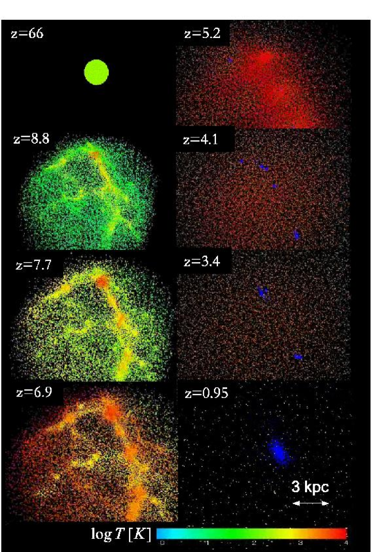
Figure 4: Time evolution of the spatial distributions of SPH and star particles for $M_{\rm halo}\simeq 6\times 10^{7}M_{\odot}$ and $z_{\rm c}\simeq 1.7$ is shown. The figure consists of 8 panels. Upper-left panel is the distribution of SPH particles at very early phase, and it evolves downward in the left column, continuing to the upper-right panel. Corresponding redshift is printed at the upper-left corner of each panel. The colors of dots represent the logarithmic temperature of the SPH particles, and the color legend is shown at the bottom in logarithmic scale, as well as the physical scale ruler (3 kpc) at the right-bottom corner. The blue particles do not represent SPH particles, but star particles.

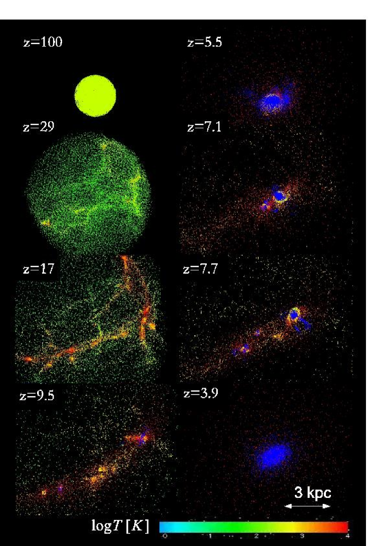
Figure 5: Same as Fig.4 except that the parameters are $M_{\rm halo}\simeq 6\times 10^{8}M_{\odot}$ and $z_{\rm c}\simeq 7.6$.

Figures 4 and 5 show two typical results, where $c_{*}=0.1$ for both cases. Figure 4 shows the low-$z_{\rm c}$ ($z_{\rm c}\simeq 1.7$) and less massive case ($M_{\rm halo}\simeq 6\times 10^{7}M_{\odot}$). Dots in the figure denote the location of SPH particles and numerically formed stars. The colors of particles represent the gas temperature (color legend is shown at the bottom), except that blue particles denote stars. At $z\simeq 66$ (1st panel), the initial condition is set in a spherical region as described in section 2.5. Thereafter, the system expands by the cosmic expansion, and also baryon perturbations are induced by imprinted dark matter fluctuations (2nd panel). At $z\simeq 9$, first objects with the mass of $\sim 10^{6-7}M_{\odot}$ form at density peaks (2nd and 3rd panels). This is consistent with the previous results by Tegmark et al. (1997) and Fuller & Couchman (2000). At $z\approx 7$, the system is reionized overall and reheated by UVB (4th panel). Then, a portion of the cooled gas that is once settled into the first objects is evaporated as a pressure-driven thermal wind at $z\approx 5$ (5th panel). But a significant amount of baryons are self-shielded against UVB at high-density peaks even during the reionization, so that the photoheating is precluded deep inside the peaks and eventually stars form there. As a result, small star clusters are left after the reionization epoch (6th panel). The stellar clusters coalesce with each other in a dissipationless fashion, according as dark matter fluctuations grow hierarchically (7th panel). Finally, a subgalactic spheroidal system with a high total mass-to-stellar mass ratio ($M_{\rm halo}/M_{\rm star}=20$) forms. If we assume the stellar mass to luminosity ratio of 3 in solar units that comes from a Salpter-like initial mass function, then the mass-to-light ratio of this system is assessed to be $M_{\rm halo}/L=63$.

In the above case, baryons are cooled to form stars only at density peaks, and gas in other regions is photoevaporated, resulting in a thermal wind. But, the evolution is quite different for the high-$z_{\rm c}$ and massive halo model. Figure 5 represents the $z_{\rm c}\simeq 7.6$ and $M_{\rm halo}\simeq 6\times 10^{8}M_{\odot}$ case. In this case, most of baryons collapse before the reionization. Resultantly, the photoevaporation is less effective than the low-$z_{\rm c}$ case, and thus the whole system does not lose a significant portion of baryonic matter. Finally, a formed spheroidal system has $M_{\rm halo}/M_{\rm star}=7.7$, which is close to the assumed initial the total mass-to-baryonic mass ratio, $\Omega/\Omega_{\rm B}=7.35$. The mass-to-light ratio of this system is assessed to be $M_{\rm halo}/L=26$.

3.2 Star Formation History

In Figure 6, the star formation histories (SFH) are shown for typical four runs, which are the low mass ($6\times 10^{7}M_{\odot}$) case with $z_{\rm c}=1.7$ and 8.1 and the high mass ($6\times 10^{8}M_{\odot}$) case with $z_{\rm c}=1.1$ and 7.6. As commonly seen, the SFR is peaked before $10^{9}$yr ($z\gtrsim 5$) and the star formation activity is substantially suppressed by UVB after the reionization, $z\lesssim 5$. This indicates that the star formation mainly occurs in high-density regions which collapsed prior to the reionization. The peak SFR is lower in the systems with lower collapsing epochs. However, the difference is not so drastic. The peak SFR in $z_{\rm c}\approx 1$ cases is roughly a half of that in $z_{\rm c}\approx 8$ cases. If based on the criterion for spherical clouds (e.g. Kitayama et al. 2001), the clouds should be completely photoevaporated in the two cases of $z_{\rm c}\approx 1$. But, the present results show that high-density peaks which collapse before the reionization contribute significantly to the star formation even in such low-$z_{\rm c}$ objects. This is a consequence of the hierarchical growth of density fluctuations that is caused by the CDM spectrum.

As another important result, it should be noted that the star formation activity in the case with $M_{\rm halo}\simeq 6\times 10^{8}M_{\odot}$ for high-$z_{\rm c}$ continues even after the reionization. This is caused by the depth of gravitational potential. A massive galaxy with high-$z_{\rm c}$ has a deeper gravitational potential. Thus, the dark halo can prevent the photoheated gas from blowing out into the intergalactic space. Instead, the heated gas slowly accretes in the potential of dark halo. Eventually, the gas is self-shielded from UVB and cools by H₂, so that stars form even in UVB.

In Figure 7, the final fraction of stars, $f_{\rm star}$, is plotted against collapse epoch $z_{\rm c}$, where $f_{\rm star}$ is defined by the total mass of star particles divided by the total baryonic mass at $z=1$ ($f_{\rm star}\equiv M_{\rm star}/M_{\rm baryon}$). The starred pentagons represent the results of $M_{\rm halo}\simeq 6\times 10^{8}M_{\odot}$ runs, and the pentagons denote those of $M_{\rm halo}\simeq 6\times 10^{7}M_{\odot}$ runs, where $c_{*}$ is assumed to be $0.1$. The stellar fraction is smaller for $M_{\rm halo}\simeq 6\times 10^{7}M_{\odot}$ cases than $M_{\rm halo}\simeq 6\times 10^{8}M_{\odot}$ cases. This comes from the SFH shown above. The massive objects tend to retain more gas components than less massive objects in the presence of UVB.

Additionally, $f_{\rm star}$ decreases monotonously with decreasing $z_{\rm c}$ for both $M_{\rm halo}\simeq 6\times 10^{8}M_{\odot}$ and $M_{\rm halo}\simeq 6\times 10^{7}M_{\odot}$ cases. It is found that the dependence of $f_{\rm star}$ on $1+z_{\rm c}$ is almost linear, and its relation is given by

$$f_{\rm star}\simeq a(M)\left(1+z_{\rm c}\right)+b(M)$$ (14)

where $a(6\times 10^{8}M_{\odot})=7.7\times 10^{-2}$, $a(6\times 10^{7}M_{\odot})=6.9\times 10^{-2}$ , $b(6\times 10^{8}M_{\odot})=0.26$ and $b(6\times 10^{7}M_{\odot})=7.7\times 10^{-2}$. We emphasize that even for galaxies assembled after the reionization, some fraction of baryons are cooled and form stars at high-density peaks. The vertical two lines denote the critical redshifts obtained by Kitayama et al. (2001), after which protogalactic clouds are photoevaporated. The condition for $M_{\rm halo}\simeq 6\times 10^{7}M_{\odot}$ is denoted by a solid line and that for $M_{\rm halo}\simeq 6\times 10^{8}M_{\odot}$ by a dotted line. This result shows again that the inhomogeneity in protogalactic clouds is crucial for the star formation in them, because a portion of baryons collapse and cool before the reionization, and also some fraction of gas is self-shielded from UVB even after the reionization if the gas accretes in dark matter potential.

In Figure 7, we plotted also the results with $c_{*}=1$ (high SFR runs) and $c_{*}=0.01$ (low SFR runs). As seen clearly, the results are basically the same as the case of $c_{*}=0.1$. This is physically understood as follows: In the present simulations, stars form from overdense regions with $\rho\gtrsim 10^{-22}{\rm g~{}cm^{-3}}$. Then, the star formation timescale assessed by the present star formation algorithm (12) is given by $t_{\rm SF}=t_{\rm ff}/c_{*}\lesssim 10^{7}~{}c_{*}^{-1}{\rm yr}$. On the other hand, the UV feedback is quite effective at $z\lesssim 5$ which corresponds to $t_{\rm H}\gtrsim 10^{9}{\rm yr}$. Thus, the main episode of the initial star formation ends before the reionization as far as $c*\gtrsim 0.01$. Moreover, the density of star forming regions is higher if $c_{*}$ is smaller, because further radiative cooling works before the gas is converted to stars. Therefore, the local free-fall time of star forming region is shorter for smaller $c_{*}$. Consequently, $c_{*}$ is not so important to determine the final stellar fraction. However, if we adopt $c_{*}=0.01$, the star formation history is modified as a matter of course. The epoch of star formation is shifted to later epoch for $c_{*}=0.01$, as shown in Fig.8. Especially, in the cases with high mass and high-$z_{\rm c}$, the star formation activity after the reionization is enhanced compared to the $c_{*}=0.1$ case. The relation of this result to the continuous star formation history inferred in nearby dwarf galaxies (e.g. Mateo 1998) will be discussed later.

3.3 Radiative Transfer Effect

Here, we show more specifically the effects of radiative transfer in the present simulations. For comparison, we perform the control runs in which gas is assumed to be optically thin against UV radiation. In Figure 9, the time variations of stellar fractions are compared between the runs with and without radiative transfer. The parameters are the same as those in Figure 6. For all runs, it is clear that the star formation activities are supressed at earlier epochs and thoroughly terminated after the reionization in optically-thin simulations. In Figure 10, the final stellar fractions ($f_{\rm star}$) are shown for the runs with and without radiative transfer. The optically-thin approximation underestimates the stellar fraction by a factor of 1.5-2 for all runs in the $z_{\rm reion}\simeq 7$ models, regardless of the mass and collapse epoch. The radiative transfer effect is even more crucial in $z_{\rm reion}\simeq 17$ models as shown in §3.5 below. The reduction of $f_{\rm star}$ by dismissing the radiative transfer is more than an order of magnitude if $z_{\rm reion}\simeq 17$. Hence, it is clear that the self-shielding does work to form stars effectively during the reionization.

Also, in the bottom-right panel of Figure 9, where $M_{\rm halo}\simeq 6\times 10^{8}M_{\odot}$ and $z_{\rm c}=7.6$, $f_{\rm star}$ continues to increase if the radiative transfer is incorporated. Since the gravitational potential is as deep as to sustain the photoheated gas in this case, some gas is self-shielded in the course of accretion onto local density peaks, so that stars continue to form. In the optically-thin simulation, the accreted gas cannot be cooled below $10^{4}$K owing to the absence of shielding effect, so that no stars form after the reionization.

3.4 Kinematic Properties

In Table 1, 1D velocity dispersion of the formed stars ($\sigma_{\rm 1D}$) and effective size $R_{\rm half}$ of the resultant spheroidal system are listed for various runs. Here, the effective size, $R_{\rm half}$, is defined so that a half of stars are contained within the radius. In the low-$z_{\rm c}$ case shown in Figure 4, gas can cool at density peaks before the reionization and form compact star clusters. The star clusters coalesce in a dissipationless fashion to form a single spheroidal system eventually. On the other hand, in the high-$z_{\rm c}$ case as shown in Figure 5, the formation process of the final stellar system is rather different, because the star formation proceeds not only at the density peaks but also after the collapse of the whole system, which takes place after the reionization. In order to clarify the difference quantitatively, we plot the time variation of the ratio of the total kinetic energy by random motion ($E_{\rm ran}$) to the total rotation energy ($E_{\rm rot}$). Here, $E_{\rm rot}$ is defined as the summation of the rotational energy of baryonic particles (i.e. SPH particles and star particles) which is contained in a sphere with radius of $R_{vir}(z)$ from the center of gravity;

$$E_{\rm rot}=\sum_{r_{\rm i}<R_{\rm vir}(z)}\frac{1}{2}m_{\rm i}v_{\rm rot,i}^{2},$$ (15)

where $v_{\rm rot,i}$ is the angular velocity of i-th particle. $E_{\rm ran}$ is defined by the rest of the kinetic energy, that is, $E_{\rm ran}=E_{\rm kin}-E_{\rm rot}$, where $E_{\rm kin}$ is the total kinetic energy. When the velocity field is isotropic, the ratio $E_{\rm rot}/E_{\rm ran}$ should be $1/5$ according to the present definition. Figure 11 shows the time evolution of the ratio $E_{\rm rot}/E_{\rm ran}$ for typical four runs after the collapse epoch. As shown in this figure, $E_{\rm rot}/E_{\rm ran}$ is well below unity for all the cases after $z_{\rm c}$. This means that these systems are not rotationally supported. However, if we take a closer look, the ratio for the high-mass and high-$z_{\rm c}$ case ($M_{\rm halo}\simeq 6\times 10^{8}M_{\odot},z_{\rm c}\simeq 7.6$) is somewhat larger than the others. This reflects the fact that a part of gas forms a rotating disk before it is converted into stars. On the other hand, for the other cases, gas is lost after the reionization era ($z\lesssim 7$), and no rotating disc forms.

3.5 Effects of Early Reionization

Here, we attempt to evaluate the effects of early reionization as inferred by the results of WMAP (Kogut et al., 2003). We perform two runs in the high-$z$ reionization regime ($z_{\rm reion}\approx 17$) described at the end of §2.5. The both runs are high-$z_{\rm c}$ models, where $M_{\rm halo}\simeq 6\times 10^{7}M_{\odot}$ with $z_{\rm c}=8.1$ or $M_{\rm halo}\simeq 6\times 10^{8}M_{\odot}$ with $z_{\rm c}=7.6$. The star formation history and the time evolution of stellar fractions are shown in Figure 12. First, for the former run ($M_{\rm halo}\simeq 6\times 10^{7}M_{\odot}$), the effects of early reionization feedback are noticeable, and the fraction of stellar component becomes roughly four times smaller than the fiducial reionization regime ($z_{\rm reion}\approx 7$). Nonetheless, some fraction of baryons are cooled to form stars even at $z<17$, owing to the effects of self-shielding. This is partly because the intergalactic medium is not perfectly transparent to UVB, even if the UV intensity is strong enough to reionize the universe (Nakamoto, Umemura, & Susa, 2001). On the other hand, for the latter run ($M_{\rm halo}\simeq 6\times 10^{8}M_{\odot}$), the final stellar fraction is smaller than the fiducial model, but the effect is not so drastic as the former case. In this case, the final fraction of stars is $\sim 20\%$ smaller than the fiducial model.

We also stress that the effect of radiation transfer is very important for such early reionization model. In the lower panels of Figure 12, the results from the optically-thin simulations are also plotted by dashed curves. It is quite clear that the star formation is almost prohibited if the optically thin is assumed, where the final stellar fraction is reduced by an order of magnitude. The results of more systematic investigation will be reported in a forthcoming paper.

4 Discussion

4.1 Substructure Problem

Recent numerical simulations predict that subgalactic dark halos are overabundant compared to dwarf spheroidals observed around our Galaxy (Moore et al., 1999). So far, the possibility that this substructure problem might be reconciled if the star formation is significantly suppressed by UVB in subgalactic halos has been discussed extensively. However, the present simulations have shown that the suppression by UVB is not complete. Especially, even in the early reionization regime, the photoevaporation by UVB is not complete and the effects of self-shielding are still significant. Hence, in the context of CDM cosmology, some fraction of baryons forms stars inevitably. Thus, we have to take into account the shelf-shielding properly, in order to evaluate the effects of UVB feedback on substructure problem.

To make a further approach on this problem, other effects such as the internal UV sources, the evaporation driven by SN explosions with the strongly top-heavy initial mass function of formed stars or the gas tripping in intracluster medium may have to be investigated.

4.2 dE/dSph’s in Local Group

What objects correspond to the simulated galaxies? One possibility is dE/dSph galaxies in the Local Group (LG). The dwarf galaxies in LG are known to be extended (low surface brightness), spheroidal system (e.g. Mateo 1998). Especially, faint dSph’s ($M_{V}\gtrsim-14$) have a larger mass-to-light ratio. Hirashita, Takeuchi, & Tamura (1998) have found

$$\log(M_{\rm vir}/L)=2.0\log M_{\rm vir}+13.1$$ (16)

for $M_{\rm vir}<10^{8}M_{\odot}$, while $\log(M_{\rm vir}/L)\simeq 0.4-0.7$ for $M_{\rm vir}>10^{8}M_{\odot}$. These observational features indicate that the mass loss is more prominent for $M_{\rm vir}<10^{8}M_{\odot}$. This can be attributed to SN-driven winds (Hirashita, Takeuchi, & Tamura, 1998; Mori, Ferrara, & Madau, 2002). The present numerical simulations suggest that such a wind can occur also by the photoheating due to the reionization, even before SN explosions drive a thermal wind. If we use the final stellar fraction (14), we find $M_{\rm halo}/L=63$ with assuming $M_{\rm star}/L=3$ for $z_{\rm c}=1.7$ and $M_{\rm halo}\simeq 6\times 10^{7}M_{\odot}$. Such a high M/L is also obtained by the recent results by Ricotti (2003) in which 3D cosmolgical radiation hydrodynamical simulations are performed with OTVET approximation (Gnedin & Abel, 2001). We also remark that Shaviv & Dekel (2003) pointed out the connection between dSphs and photoevapolated galaxies with 1D simulations.

In addition, the SFH in the Local Group dwarfs has a ubiquitous feature (e.g. Mateo 1998; Gnedin 2000a). The stars in most LG dwarfs are estimated to have formed more than 10 Gyrs ago. This means that star formation rate should have a clear cut-off at such epoch. If we assume the age of the universe is 13 Gyr, 10 Gyr in lookback time corresponds to $z\sim 3$, which is 2 Gyrs later than the cut-off epoch ($z\sim 4-5$) in the present simulations. However, the observed star formation history itself should have uncertainties of a few Gyrs. Thus the reheating by reionization could be one of the promising mechanism to provide such a cut-off in SFH of the LG dwarf galaxies. Also, the SFH in the LG dwarfs has another important feature: there still remain weak star formation activities after the cut-off of star formation rate. This feature may be reproduced by the numerical galaxies presented here, if $c_{*}$ is at a level of 0.01 for relatively high mass and high-$z_{\rm c}$ models (see §3.2). Furthermore, if one incorporates the recycling of gas ejected from the stars, which is not included in the present simulation, additional stars may form unless the compete evaporation does not occur. This tendency is expected to be conspicuous for the halos with a deep gravitational potential. However, the gas ejected to the intersteller space in such dwarf galaxeis will be photoionized again. The effects of self-shielding and the formation of dust will delay the photoevaporation of the processed gas and consequently some amount of gas will be converted into stars again.

4.3 dIrr’s in Local Group

On the other hand, the observed dIrr’s in LG still have significant star formation activities embedded in old extended spheroidal components. Although we have no counterpart in the present simulations, we can infer the origin of such galaxies by extrapolating the numerical results. Massive ($\sim 10^{10}M_{\odot}$) halos formed at low $z_{\rm c}$ might be the candidate of such galaxies. In such halos, small scale perturbations grows slowly. Thus, the fraction of gas component after the reionization of the universe is large as seen in Figure 7. In addition, such halos have a gravitational potential deep enough to sustain photoionized gas, so that stars form efficiently from such abundant gas. Therefore, active star formation is expected even after the reionization. We can suggest that the conditions requisite for dIrr formation are 1) that the gravitational potentials of dark halos are deep enough to retain photoheated gas, and 2) that the galaxy formation epoch is later than the reionization epoch. Actually, dIrr’s appear to be rather massive (e.g. Mateo 1998). Also, the reduction of star formation rate due to UVB may suppresses the SN-driven galactic wind and thereby allows the formation of diffuse dwarf systems like Irr’s.

5 Conclusions

In this paper, we have performed 3D radiation hydrodynamic simulations on the formation of low-mass objects under UVB. The suppression by UVB of the formation of low-mass objects at lower redshifts ($M\lesssim 10^{9}M_{\odot},z_{\rm c}\lesssim 5$) is confirmed. But, simultaneously it is found that the formation of low-mass galaxies at low redshifts is not completely forbidden by the UVB-induced photoevaporation. Baryons at high-density peaks can collapse and be self-shielded from UVB even during the reionization, to form stars eventually. This occurs even if the universe was reionized at earlier epochs as suggested by the WMAP. Thus, effects of UVB feedback on the substructure problem with a cold dark matter (CDM) scenario should be evaluated with careful treatment of the radiative transfer.

In order to clarify the effects of radiative transfer, we have compared the results of simulations with those under the assumption of optically-thin medium.

The reduction for the final stellar fraction is 30-40% without radiative transfer in the $z_{\rm reion}\simeq 7$ regime. Hence, the star formation before the reionization is important to determine the final stellar fraction. But, the radiative transfer effect is much more serious in the earlier reionization ($z_{\rm reion}\simeq 17$) regime, where the reduction for the final stellar fraction is more than an order of magnitude. Also, it should be stressed that in the optically-thin approximation, gas temperature of the cloud becomes always higher than $10^{4}$ K after the reionization, so that stars cannot form there, whereas the self-shielding arising from radiative transfer allows star formation even after the reionization if the gravitational potential is deep enough to retain the gas. The star formation after the reionization must influence the subsequent evolution of dwarf galaxies with the possible recycling of interstellar matter.

In the previous optically-thin simulations (e.g. Tassis et al. 2003), the star formation criterions are different from those in the present simulation. The conditions used here are stricter than those used in the previous works. In previous simulations, stars can form slowly even after the reionization due to the milder star formation conditions, although the cold HI regions cannot be formed. Although such a treatment of star formation might be approximately valid, it should be confirmed by the simulations with radiative transfer.

We also have investigated the effects of $c_{*}$, and found that the final stellar fractions are not so different for various values of $c_{*}$. However, a smaller value of $c_{*}$ delays star formation and allows enhanced star formation after the reionization if the system is relatively massive and the collapse epoch is considerably later the reionization. Also, if the stellar feedback is taken into account, the further effects of $c_{*}$ may be expected, since 1) larger $c_{*}$ results in faster recycling (i.e. a larger amount of heavy elements), and 2) larger $c_{*}$ is followed by simultaneous SN explosion, which means easier disruption of host galaxies. These issue should be investigated by the simulations that take into account the stellar feedback coupled with radiative transfer.

The star clusters formed at high-density peaks coalesce with each other in a dissipationless fashion to form a spheroidal system with a large mass-to-light ratio. It is also found that there is a sharp cut-off of star formation rate at $z\simeq 4-5$ in all the simulations because of the appreciable photoevaporation of cold gas clouds in the reionized universe. Moreover, in massive dwarf galaxies ($M_{\rm halo}\simeq 6\times 10^{8}M_{\odot}$) formed at high redshifts ($z_{\rm c}\sim 8$), weak star formation activities continue even after the reionization. On the other hand, less massive ($M_{\rm halo}\simeq 6\times 10^{7}M_{\odot}$) galaxies formed later ($z_{\rm c}\lesssim 8$) do not have star formation activities after $z\simeq 4-5$. Observational counter parts of these systems might be the dwarf spheroidal galaxies in the Local Group. Those galaxies have extended, old and spheroidal stellar systems, with characteristic star formation histories. It is also known that fainter galaxies have larger mass-to-light ratio. All of those features agree qualitatively with those of the simulated galaxies, although the stellar feedback should be also investigated to make quantitative comparison with observed galaxies.

Table 1: Properties of Formed Galaxies

$z_{\rm c}$	$M_{\rm halo}/M_{\odot}$	$T_{\rm vir}/$K	$\sigma_{\rm 1D}/{\rm km~{}s^{-1}}$	$\sigma_{\rm 1D}({\rm DM})/{\rm km~{}s^{-1}}$	$R_{\rm half}/{\rm pc}$	$f_{\rm star}$	$M_{\rm halo}/L$
1.7	$5.9\times 10^{7}$	$3.6\times 10^{3}$	$4.6$	$5.5$	$62$	0.28	63
3.4	$5.9\times 10^{7}$	$5.1\times 10^{3}$	$5.1$	$6.5$	$58$	0.37	50
5.1	$6.1\times 10^{7}$	$6.3\times 10^{3}$	$5.7$	$7.2$	$69$	0.47	44
6.5	$6.1\times 10^{7}$	$8.2\times 10^{3}$	$6.4$	$8.2$	$66$	0.61	36
8.1	$6.1\times 10^{7}$	$1.0\times 10^{4}$	$7.1$	$9.2$	$62$	0.71	33
1.1	$6.0\times 10^{8}$	$1.7\times 10^{4}$	$14$	$12$	$2.9\times 10^{2}$	0.43	40
2.9	$6.0\times 10^{8}$	$2.0\times 10^{4}$	$16$	$14$	$2.1\times 10^{2}$	0.55	31
4.5	$6.0\times 10^{8}$	$2.0\times 10^{4}$	$17$	$16$	$2.2\times 10^{2}$	0.68	31
6.0	$6.1\times 10^{8}$	$2.1\times 10^{4}$	$19$	$19$	$1.8\times 10^{2}$	0.79	29
7.6	$6.1\times 10^{8}$	$2.6\times 10^{4}$	$20$	$21$	$1.6\times 10^{2}$	0.93	26

Figure 1: H₂ Cooling functions induced by H-H₂ collision are plotted against the temperature for two different densities. Solid curves are plotted based upon the formula given by Hollenbach & McKee (1979), long dashed curves by Galli & Palla (1998) and the short dashed curves by Lepp & Shull (1983). They are discrepant at low density. In this paper, those by Galli & Palla (1998) are adopted.

Figure 2: Cooling functions below $10^{4}$K are plotted. Two solid lines denote the cooling rate due to metals, assuming $Z/Z_{\odot}=1$ and $10^{-2}$ respectively. H₂ cooling function is plotted for the postshock region with shock velocity larger than 30 km/s (dotted line) and also for a given abundance of $y_{\rm H_{2}}=10^{-4}$ (short dashed line). A long dashed line represents the rate by hydrogen Ly $\alpha$.

Figure 6: The time-variation of star formation rate (SFR) is plotted against the cosmic time. Four panels represent respectively the results of four different runs, where the parameters are displayed in each panel. The vertical short dashed lines denote $z=7$ and $z=6$, between which the reionization is almost completed in this model.

Figure 7: The final stellar fraction $f_{\rm star}$ is plotted against the collapse redshift. Each mark denotes the result of a run: pentagons($c_{*}=1$), squares($c_{*}=0.1$), and triangles($c_{*}=0.01$) denote the runs with $M_{\rm halo}\simeq 6\times 10^{7}M_{\odot}$. Similarly, starred pentagons($c_{*}=1$), starred squares($c_{*}=0.1$), and starred triangles($c_{*}=0.01$) represent the results of relatively massive galaxies ($M_{\rm halo}\simeq 6\times 10^{8}M_{\odot}$).

Figure 8: Same as Fig. 6, except that $c_{*}=0.01$.

Figure 9: The time-variations of stellar fraction $f_{\rm star}$ are plotted against the cosmic time for transfer and optically-thin cases. Solid lines are the results with radiative transfer, while dashed lines are those under the assumption of optically-thin. Parameters of four panels are the same as that in Fig.6. The vertical short dashed lines denote $z=7$ and $z=6$, between which the reionization is almost completed in this model.

Figure 10: The final stellar fraction $f_{\rm star}$ is compared between radiative transfer and optically-thin cases, assuming $c_{*}=0.1$. Filled symbols represent the results of full radiative transfer simulations, and open symbols denote the results of optically-thin simulations.

Figure 11: The rotation energy-to-random motion energy ratio ($E_{\rm rot}/E_{\rm ran}$) is plotted against the cosmic time. Parameters of four panels are the same as that in Fig.6. Spikes in this figure come from merger of subclumps. Since $E_{\rm rot}$ and $E_{\rm ran}$ are measured from the center of gravity (see the text), violent mergers cause high spikes. Especially, in the left panels, the collapse epoch is relatively late, so that such violent merger phases are conspicuous.

Figure 12: Star formation histories in the early reionization regime are shown (upper two panels), and time evolutions of stellar fraction are shown by the solid curves (lower two panels). The parameters are attached in each panel. The results of optically-thin simulations are also shown in the lower two panels (dashed curve). In these simulations, $c_{*}=0.1$ is assumed. The vertical short dashed lines denote $z=17$ and z=16, between which the reionization is almost completed in this early reionization model.

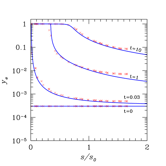
Figure 13: Propagation of ionization front is shown (see also the text). Crosses denote the numerical results, while solid lines are analytic solution.

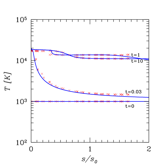
Figure 14: Same as Fig.13, except that the vertical axis denotes gas temperature.

References

- Abel, Norman & Madau (1999) Abel, T., Norman, M. & Madau, P. 1999, ApJ, 523, 66
- Babul & Rees (1992) Babul, A. & Rees, M. J. 1992, MNRAS, 255, 346
- Bajtlik, Duncan, & Ostriker (1988) Bajtlik, S. Duncan, R. C., & Ostriker, J. P. 1988, ApJ, 327, 570
- Binney, Gerhard, & Silk (2001) Binney, J., Gerhard, O., & Silk, J. 2001, MNRAS, 321, 471
- Boku et al. (2002) Boku, T., Makino, J., Susa, H., Umemura, M., Fukushige, T. & Ukawa, A. 2002, IPSJ Transactions on High Performance Computing Systems, 41, 5
- Bromm et al. (2001) Bromm, V., Ferrara, A., Coppi, P. S. & Larson, R. B. 2001, MNRAS, 328, 969
- Cen & Ostriker (1993) Cen, R. & Ostriker, J. P. 1993, ApJ, 417, 404
- Cole et al. (1994) Cole, S., Aragon-Salamanca, A., Frenk, C. S., Navarro, J. F., & Zepf, S. E. 1994, MNRAS, 271, 781
- Corbelli, Galli & Palla (1997) Corbelli, E., Galli, D & Palla, F. 1997, ApJ, 487, 53L
- Dalgarno & McCray (1972) Dalgarno, A. & McCray, A. 1972, ARA&A, 10, 375
- Dekel & Rees (1987) Dekel, A. & Rees, M. J. 1987, Nature, 326, 455
- Djorgovski, Castro, Stern, & Mahabal (2001) Djorgovski, S. G., Castro, S., Stern, D., & Mahabal, A. A. 2001, ApJ, 560, L5
- Dove & Shull (1994) Dove, J. B., & Shull, M. 1994, ApJ, 423, 196
- Efstathiou (1992) Efstathiou, G. 1992, MNRAS, 256, 43P
- Ferrara & Tolstoy (2000) Ferrara, A. & Tolstoy, E. 2000, MNRAS, 313, 291
- Fuller & Couchman (2000) Fuller, T. M. & Couchman, H. M. P. 2000, ApJ, 544, 6
- Galli & Palla (1998) Galli D. & Palla F. 1998, A&A, 335, 403
- Giallongo et al. (1996) Giallongo, E., Cristiani, S., D’Odorico, S., Fontana, A., & Savaglio, S. 1996, ApJ, 466, 46
- Gnedin (2000a) Gnedin, N. Y 2000a, ApJ, 535, 75L
- Gnedin (2000b) Gnedin, N. Y. 2000b, ApJ, 535, 530
- Gnedin (2000c) Gnedin, N. Y. 2000c, ApJ, 542, 535
- Gnedin & Abel (2001) Gnedin, N. Y. & Abel, T. 2001, NewA, 6, 437
- Heavens & Peacock (1988) Heavens, J.A. & Peacock, A.F., 1988, MNRAS, 232, 339
- Hirashita, Takeuchi, & Tamura (1998) Hirashita, H., Takeuchi, T. T., & Tamura, N. 1998, ApJ, 504, L83
- Hollenbach & McKee (1979) Hollenbach, D. & McKee, F., 1979, ApJS, 41, 555
- Iwasaki (1988) Iwasaki Y. 1998, Nucl. Phys. B (Proc. Suppl.), 60A, 246
- Kang & Shapiro (1992) Kang, H., & Shapiro, P. 1992 , ApJ, 386, 432
- Kauffmann, White, & Guiderdoni (1993) Kauffmann, G., White, S. D. M., & Guiderdoni, B. 1993, MNRAS, 264, 201
- Kennicutt (1998) Kennicutt, R. C. 1998, ARA&A, 36, 189
- Kepner, Babul & Spergel (1997) Kepner, J., Babul, A., Spergel, D. 1997, ApJ, 487, 61
- Kessel-Deynet & Burkert (2000) Kessel-Deynet, O. & Burkert, A. 2000, MNRAS, 315, 713
- Kitayama et al. (2001) Kitayama,T., Susa, H., Umemura, M., & Ikeuchi, S. 2001, MNRAS, 326, 1353
- Koda, Sofue & Wada (2000) Koda, J., Sofue, Y. & Wada, K. 2000, ApJ, 532, 214
- Kogut et al. (2003) Kogut, A. et al. 2003, ApJ, submitted (astro-ph/0302213)
- Lepp & Shull (1983) Lepp, S.& Shull, M. 1983, ApJ, 270, 578L
- Makino (2002) Makino, J. 2002, ASP Conf. Ser. 263: Stellar Collisions, Mergers and their Consequences, 389
- Maloney (1993) Maloney, P. 1993, ApJ, 414, 41
- Mateo (1998) Mateo, M. 1998, ARA&A, 36, 435
- Moore et al. (1999) Moore, B., Ghigna, S., Governato, F., Lake, G., Quinn, T., Stadel, J., & Tozzi, P. 1999, ApJ, 524, L19
- Mori, Ferrara, & Madau (2002) Mori, M., Ferrara, A., & Madau, P. 2002, ApJ, 571, 40
- Nakamoto, Umemura, & Susa (2001) Nakamoto, T., Umemura, M., & Susa, H. 2001, MNRAS, 321, 593
- Nishi & Susa (1999) Nishi, R. & Susa, H. 1999, ApJ, 523, L103
- Omukai (2000) Omukai, K. 2000, ApJ, 534, 809
- Razoumov et al. (2002) Razoumov, A. O., Norman, M. L., Abel, T., & Scott, D. 2002, ApJ, 572, 695
- Ricotti, Gnedin, & Shull (2002a) Ricotti, M., Gnedin, N. Y., & Shull, J. M., 2002a, ApJ, 575, 33
- Ricotti, Gnedin, & Shull (2002b) Ricotti, M., Gnedin, N. Y., & Shull, J. M., 2002b, ApJ, 575, 49
- Ricotti (2003) Ricotti, M. 2003, ASSL Conference Proceedings 281: The IGM/Galaxy Connection, 193
- Schneider et al. (2002) Schneider, R., Ferrara, A., Natarajan, P., & Omukai, K. 2002, ApJ, 571, 30
- Shapiro & Raga (2001) Shapiro, P. R. & Raga, A. C., 2001, The Seventh Texas-Mexico Conference on Astrophysics: Flows, Blows and Glows, Revista Mexicana de Astronomia y Astrofisica (Serie de Conferencias) 10, 109
- Shaviv & Dekel (2003) Shaviv, N. J. & Dekel, A. 2003, astro-ph/0305527
- Songaila (2001) Songaila, A. 2001, ApJ, 561, 153L
- Steinmetz & Bartelmann (1995) Steinmetz, M. & Bartelmann, M., 1995, MNRAS, 272, 570
- Steinmetz & Müller (1993) Steinmetz, M. & Müller, E. 1993, A&A, 268, 391
- Sugimoto et al. (1990) Sugimoto, D., Chikada, Y., Makino, J., Ito, T., Ebisuzaki, T., & Umemura, M. 1990, Nature, 345, 33
- Susa & Kitayama (2000) Susa, H. & Kitayama, T. 2000, MNRAS, 317, 175
- Susa & Umemura (2000) Susa, H. & Umemura, M. 2000, ApJ, 537, 578
- Susa & Umemura (2000) Susa, H. & Umemura, M. 2000, MNRAS, 316, L17
- Tajiri & Umemura (1998) Tajiri, Y. & Umemura, M. 1998, ApJ, 502, 59
- Tassis, Abel, Bryan & Norman (2003) Tassis, K., Abel, T., Bryan, G. & Norman, M. 2003, ApJ, in press (astro-ph/0212457)
- Tegmark et al. (1997) Tegmark, M., Silk, J., Rees, M. J., Blanchard, A., Abel, T., & Palla, F. 1997, ApJ, 474, 1
- Thacker et al. (2000) Thacker, J., Tittley, R., Pearce, R., Couchman, P. & Thomas, A. 2000, MNRAS319, 619
- Thoul & Weinberg (1996) Thoul, A. A. & Weinberg, D. H. 1996, ApJ, 465, 608
- Umemura & Ikeuchi (1984) Umemura, M. & Ikeuchi, S. 1984, Progress of Theoretical Physics, 72, 47
- Umemura et al. (1993) Umemura, M., Fukushige, T., Makino, J., Ebisuzaki, T., Sugimoto, D., Turner, E. L., & Loeb, A. 1993, PASJ, 45, 311
- Umemura (1993) Umemura, M. 1993, ApJ, 406, 361
- Umemura, Nakamoto, & Susa (2001) Umemura, M., Nakamoto, T., & Susa H. 2001, ASP Conf. Ser. 222: The Physics of Galaxy Formation, 109
- White & Frenk (1991) White, S. D. M. & Frenk, C. S. 1991, ApJ, 379, 52
- Young & Lo (1997a) Young, M. & Lo, Y. 1997, ApJ, 476, 127
- Young & Lo (1997b) Young, M. & Lo, Y. 1997, ApJ, 490, 710