Population synthesis modeling of the X-ray background with genetic algorithm – based optimization method

Abstract

We present population synthesis modeling of the X-ray background with genetic algorithm – based optimization method. In our models the best fit could be achieved for lower values of high-energy exponential cut-off ($\approx 170~{}keV$) and larger amount of the highly obscured ($\log N_{H}=25.5$) AGNs.

1 Introduction

The cosmic X-ray background (XRB) above $\sim 1$ keV is known to be produced by integrated emission of discrete sources [26, 13, 24]. The resent best reviews in this area are [7] and [14]. XRB synthesis models are usually based on the so-called unification scheme for AGN [1], which explains the different observational appearances by the orientation of accretion disk and molecular torus surrounding the nucleus. The intersection of the line of sight with the torus determines a type 2 AGNs, and the direct observation of the nucleus identifies a type 1 AGNs.

The last works in the area of population synthesis modeling used assumption about extra quantity of absorbed AGNs at high redshifts [30, 9, 28, 10, 23]. These models give good approach to the exist observations in the energy range of $1\div 100$ kev.

However, there are many unresolved yet problems exist, like as a role of the soft X-ray excess in AGN spectra at high redshifts, behaviour of the AGN luminosity function [14], possible flattening of the spectra of AGNs at high redshifts and a role of the high luminosity obscured AGNs. Furthermore, we do not have yet detailed information about an exponential cut-off at high energies.

Here we present population synthesis models of the X-ray background in order to investigate some additional conditions to obtain the best fit.

2 Fitting method

In our work we have tested one of the newest effective fitting techniques: a genetic algorithm – based optimization [3]. This method implements the Darvin’s natural selection law for the mathematical problems.

The main steps of this technique are:

1. Constructing a random initial population of the sets of the model parameters and evaluating the fitness of its members. 2. Constructing a new population by breeding selected individuals from the old population. 3. Evaluating the fitness of each member of the new population. 4. Replacing the old population by the new population. 5. Test convergence: unless fittest phenotype matches target phenotype within tolerance, goto 2.

The breeding consists of the several steps such as crossover (as a result the offspring obtains the properties of the both its parents) and mutation (which allows to probe the alternative sets of the model parameters. This option especially important, when population members become practically identical).

This method already was implemented as one of the XSpec fitting methods and now often used for different complicated fitting problems.

3 Description of the model

As for any population synthesis model, the resulting spectrum was calculated as a mix of the AGN spectra, which are typical for the different classes of AGNs, integrated over redshift and luminosity. To avoid a contribution of the Galactic diffuse radiation component, we have modeled the energy range above 1.5 keV only.

Thus, following [4], for AGN spectra we have the next expressions:

$$F(Quasars~{}1)\propto E^{-\alpha_{h}}*\exp(-\frac{E}{E_{c}})$$ (1)

$$F(Seyferts~{}1)\propto E^{-\alpha_{h}}*\exp(-\frac{E}{E_{c}})+F_{refl}(E)$$ (2)

$$F(Type~{}2)\propto F(Type~{}1)*\exp(-\sigma_{E}*N_{H})$$ (3)

where the hard energy index $\alpha_{h}=0.9$. For the exponential cut-off as a base value we have used $E_{c}=320~{}keV$, but in different models we have tried another values.

The term $F_{refl}(E)$ represents the Compton reflection component by the accretion disk and has been evaluated following [17] assuming inclination angle of $60^{\circ}$.

For obscured (type 2) AGNs, photoelectric absorption cross sections for given hydrogen column $N_{H}$ were calculated following [25]. As the base distribution of equivalent hydrogen column densities $N_{H}$ was taken from [29] (RMS hereafter). Following [18], the local ratio of absorbed and unabsorbed AGNs is $R=4.0\pm 0.9$. To evaluate this ratio with redshift, we have used the next formula

$$R(z)=\left(R(0)+\Delta R(\infty)*\left(1-\frac{1}{1+z/z_{r}}\right)\right)\times$$

$$\quad\times\exp(-z/z_{e})$$

which in contrast to the ”power law & constant” form of [10] has continuous first derivative and is convenient to represent the ratio dependence from the redshift. Here $(R(0)+\Delta R(\infty))$ is the ratio at ”infinity” and $z_{r}$ is a distance for R(z) to get value $R(0)+\frac{\Delta R(\infty)}{2}$. $z_{e}$ is an exponential cut-off scale, the same as in [28].

During integration for the X-ray luminosity function we have used expression in the form presented by [21]. For all our models the Hubble constant given by $H_{0}=50~{}km~{}s^{-1}~{}Mpc^{-1}$.

We also computed contribution of the clusters of galaxies to the overall background spectrum, adopting the temperature distribution taken from [5] and cluster luminosity function of [6].

Galactic hydrogen column was taken as $N_{H}^{gal}=10^{20}~{}cm^{-2}$.

To fit our models we have used kindly provided data from different missions like as HEAO-1 A4 LED and A2 HED detectors [11, 12, 2], ROSAT PSPC and ASCA GIS [22, 20].

The main parameters which describe our implementation of the genetic algorithm are population number (100 members for the model with 3 free parameters and 200 members for the case of 4 free parameters), variable mutation rate (initial value is 0.005) and high selection pressure regime for a breeding of the population members. Furthermore, we have used so-called ”elitism”, when the fittest generation member is copied without alteration into the next generation. A good algorithm convergence we achieve after 40–50 iterations.

4 Results and discussion

In the present work we realized several kinds of models. A simple model $A$ was calculated using equation 4 with $\Delta R(\infty)$, $z_{r}$ and $z_{e}$ as free parameters. The best fit results presented in the Table 1. The corresponded XRB fit and $R(z)$ curve one can see in Fig.1 and Fig.2.

For the model A we have the same rapid increase of the $R(z)$ with redshift, as in work of [10] and significantly much more slower exponential decay than found by [28]. We consider that such rapid increase of $R(z)$ can not be real because it makes an observer as a particular person. The most probable mistake could be using ’as is’ the distribution of equivalent hydrogen column densities of RMS. In spite of very detailed calculations of the selection effects, their sample based on optical identifications using emission lines and, hence, can lose some highly obscured AGNs. In reality the distribution could shifts towards high values of hydrogen column densities.

In order to investigate this possibility in our model B we have used as an additional parameter the quantity of AGNs with $\log{N_{H}}=25.5$. In the Table 1 the last parameter $n_{25.5}$ was calculated as a fraction of all population of type 2 AGNs in units of the RMS fractional population value (they have used $n_{25.5}\approx 0.26$). Then new local ratio of absorbed and unabsorbed AGNs is calculated as $4.0\times(1-n_{25.5}^{old}+n_{25.5}^{new})$. You can see that our new value of $n_{25.5}$ is distinctly higher than used before. For new model values the XRB spectrum is better fitted below 50 keV but is worse above 50 keV. At the same time the $R(z)$ function becomes more smooth. The distribution of hydrogen column densities for the different cases one can see in the Fig. 3.

The main problem of our fitting curves is high bias to the data above 50 keV. In reality if we analyse the data up to 400 keV it is obvious that we do not have clear exponential cut-off profile. Assuming that data below 100 keV represents the ’true’ exponential cut-off we have tried to make the model C with $E_{C}=160~{}keV$. One can see that in this case we achieve practically ideal approach to the observations, although it demands to increase the $n_{25.5}$ parameter up to 0.93.

Table 1. The best fit parameters for different models.

model	$\Delta R(\infty)$	$z_{r}$	$z_{e}$	$n_{25.5}$
A	3.34	0.11	2.49	-
B	1.21	3.01	4.46	0.47
C	2.64	0.47	2.96	0.93

In spite of approximate character of our models we have to conclude the presence of a large amount of undetected highly obscured AGNs (with $\log N_{H}=25.5$). I our future models we are going to use more precise simulations of the spectra of absorbed AGNs and the latest results obtained for the properties of the luminosity function.

Acknowledgements. Author is thankful to Duane Gruber, Elihu Boldt, Takamitsu Miyaji and Keith Gendreau for providing of the spectral data from different missions and/or useful comments. Special thanks to G$\rm\ddot{u}$nther Hasinger and Roberto Gilli for their exciting article ”The Cosmic Reality Check”.

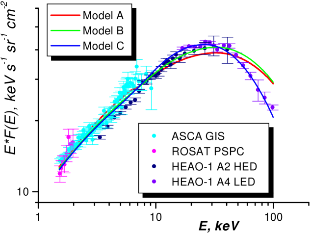
Figure 1: XRB data from different missions and our model fits.

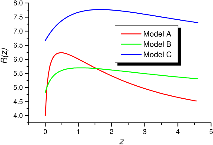
Figure 2: The ratio of absorbed and unabsorbed AGNs for different redshifts.

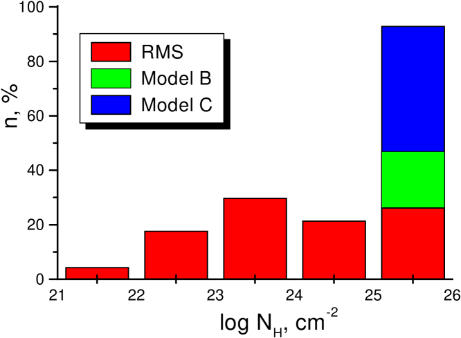
Figure 3: The distribution of the hydrogen columns of absorbed AGNs for different models and derived by [29].

References

- [1] Antonucci R.R.J., 1993, ARA&A, 31, 473
- [2] Boldt E., 2003, private communication
- [3] Charbonneau P., 1995, AJ Suppl., 101, 309
- [4] Comastri A., Setti G., Zamorani G., & Hasinger G., 1995, A&A, 296, 1
- [5] David L.P. et al., 1993, ApJ 412, 479
- [6] Ebeling H, Edge A., Fabian A., Allen S., Crawford C. & Bohringer H., 1997, ApJ 479, L101
- [7] Gilli R., 2003, astro-ph/0303115
- [8] Gilli R., Comastri A., Brunetti G. & Setti G., 1999, New Astronomy, 4, 45
- [9] Gilli R., Risaliti G. & Salvati M., 1999, A&A, 347, 424
- [10] Gilli R, Salvati M & Hasinger G., 2001, A&A, 366, 407
- [11] Gruber D., 1992, In the Proceedings of ”The X-ray background”, eds. X.Barcons & A.C.Fabian (Cambridge: Cambridge Univ. Press), p.44.
- [12] Gruber D., Matteson J., Petersen L. & Jung G., 1999, ApJ, 520, 124
- [13] Hasinger G., 2002, astro-ph/0202430
- [14] Hasinger G. and the CDF-S team, 2003, astro-ph/0302574
- [15] Iwasawa K. & Taniguchi Y., 1993, ApJ 413, L15
- [16] Loeb A. & Barkana R., 2000, ARA&A, 39, 19
- [17] Magdziarz P. & Zdziarski A., 1995, MNRAS 273, 837
- [18] Maiolino R. & Rieke G.H.,1995, ApJ 454, 95
- [19] Markevitch et al. 2003, ApJ, 583, 70
- [20] Miyaji T., 2003, private communication
- [21] Miyaji T., Hasinger G. & Schmidt M., 2000, A&A, 353, 25
- [22] Miyaji T., Ishisaki, Y., Ogasaka, Y., Ueda, Y., Freyberg, M. J., Hasinger, G. & Tanaka, Y., 1998, A&A, 334, L13
- [23] Moran E., Filippenko A. & Chornock R., 2002, ApJ, 579, 71
- [24] Moretti A, Campana S., Lazzati D., & Tagliaferri G., 2003, astro-ph/0301555
- [25] Morrison R. & McCammon D., 1983, ApJ 270, 119
- [26] Mushotzky R., Cowie L., Barger A., & Arnaud K., 2000, Nature, 404, 459
- [27] Nandra K., George L., Mushotzky R., Turner T., & Yaqoob T., 1997, ApJ 488, L91
- [28] Pompilio F., La Franca F. & Matt G., 2000, A&A, 353, 440
- [29] Risaliti G., Maiolino R. & Salvati M., 1999, ApJ 522, 157
- [30] Wilman R., & Fabian A., 1999, MNRAS, 309, 862