Intermediate Element Abundances in Galaxy Clusters

Abstract

We present the average abundances of the intermediate elements obtained by performing a stacked analysis of all the galaxy clusters in the archive of the X-ray telescope ASCA. We determine the abundances of Fe, Si, S, and Ni as a function of cluster temperature (mass) from 1 – 10 keV, and place strong upper limits on the abundances of Ca and Ar. In general, Si and Ni are overabundant with respect to Fe, while Ar and Ca are very underabundant. The discrepancy between the abundances of Si, S, Ar, and Ca indicate that the $\alpha$-elements do not behave homogeneously as a single group. We show that the abundances of the most well-determined elements Fe, Si, and S in conjunction with recent theoretical supernovae yields do not give a consistent solution for the fraction of material produced by Type Ia and Type II supernovae at any temperature or mass. The general trend is for higher temperature clusters to have more of their metals produced in Type II supernovae than in Type Ias. The inconsistency of our results with abundances in the Milky Way indicate that spiral galaxies are not the dominant metal contributors to the intracluster medium (ICM). The pattern of elemental abundances requires an additional source of metals beyond standard SN Ia and SN II enrichment. The properties of this new source are well matched to those of Type II supernovae with very massive, metal-poor progenitor stars. These results are consistent with a significant fraction of the ICM metals produced by an early generation of population III stars.

1. INTRODUCTION

Galaxy clusters provide an excellent environment for determining the relative abundances of the elements. Because clusters are the largest potential wells known, they retain all the enriched material produced by the member galaxies. This behavior is in stark contrast to our own Milky Way (Timmes, Woosley, & Weaver, 1995) and many other individual galaxies (Henry & Worthey, 1999). The accumulation of enriched material in clusters can be used as a probe to study the star formation history of the universe, the mechanisms that eject the elements into the ICM, the relative importance of different classes of supernovae, and ultimately the source of the metals in the intra-cluster medium (ICM).

The dominant baryonic component in clusters is the hot gas in the ICM, with 5–10 times as much mass as resides in the stellar component. The physics describing the dominant emission mechanism of the ICM gas is relatively simple. The ICM is optically thin, well modeled by a sphere of hydrostatic gas in thermal equilibrium, and the high temperatures and moderate densities minimize the importance of dust. Extinction, ionization, non-equilibrium and optical depth effects are minimal. As a result, cluster abundance determinations are more physically robust and reliable than those in, e.g., stellar systems, H II regions, and planetary nebulae. The hot gas emits dominantly by thermal bremsstrahlung in the X-ray band, and the strong transitions to the n=1 level (K-shell) and to the n=2 level (L-shell) of the H-like and He-like ions of the elements from carbon to nickel also lie in the X-ray band. This makes the X-ray band an attractive place for elemental abundance determinations.

Early X-ray observations of galaxy clusters (Mitchell, Culhane, Davison, & Ives, 1976; Serlemitsos et al., 1977) showed that the strong H- and He-like iron lines at 6.9 and 6.7 keV could lead to a value for the metal abundance in clusters. Later results (Mushotzky et al., 1978; Mushotzky, 1983) derived from iron line observations showed that clusters had metal abundances of about $1/3$ the solar value.

The improved spectral resolution and large collecting area of the ASCA X-ray telescope brought new power to studies of cluster metal abundances. In particular, the improved 0.5–10.0 keV energy range of ASCA allowed for better spectroscopic fits to clusters than was possible with ROSAT, which had an upper limit of 2.5 keV. Mushotzky et al. (1996) studied four bright clusters at temperatures such that strong line emission is present, and provided the first measurements of elemental abundances other than iron since the initial results from Einstein (Mushotzky et al., 1981; Becker et al., 1979; Rothenflug, Vigroux, Mushotzky, & Holt, 1984). Their measurements of silicon, neon and sulfur were interpreted as high abundances of the $\alpha$-elements in clusters. This result suggested that type II supernovae (which produce much higher $\alpha$ element yields than SN Ia) from massive stars are responsible for a significant fraction of the metals in the ICM. (Type Ia supernovae (SN Ia) produce high yields of elements in the iron peak, while Type II supernovae (SN II) produce yields rich in the $\alpha$ elements Si, S, Ne, and Mg.) Later work by Fukazawa (1997) showed that clusters are more metal enriched in their centers, and that the Si/Fe ratio is about 1.5–2.0 with respect to the solar value. Fukazawa et al. (1998) showed how the silicon abundance was higher in hotter clusters, and confirmed the importance of SN II in cluster enrichment. More recently, Finoguenov, David, & Ponman (2000), Finoguenov, Arnaud, & David (2001), and Finoguenov et al. (2002) used ASCA and XMM data to show that type Ia products dominate in the centers of certain clusters and how type II products are more evenly distributed. The observation by Arnaud et al. (1992) that the metal mass in clusters is correlated with the optical light from early type galaxies and not from spirals is also important in determining the origins of metals in the ICM.

In this paper we use the ASCA satellite (Tanaka, Inoue, & Holt, 1994) to further constrain the abundances of the intermediate elements. Previous authors referred to the elements Ne, Mg, Si, S, Ca and Ar as $\alpha$-elements in order to emphasize their supposed similar formation mechanism; we will refer to the elements observable with X-ray spectroscopy in the ASCA band as intermediate elements. This label includes nickel in the group and is preferred since the observations will show that the $\alpha$-elements do not act homogeneously as a single class.

The large database of over 300 cluster observations makes the ASCA satellite well suited for a overall analysis of the intermediate element abundances in galaxy clusters. While it is not possible to obtain accurate abundances of these elements for more than a few individual clusters, we jointly analyze many clusters at a time in several “stacks” in order to obtain the signal necessary for obtaining the abundances. The relatively large field of view of the ASCA telescope allows for spectroscopic analysis of the entire spatial extent of all but the closest clusters, and the moderate spectral resolution enables abundance determinations from the K-shell and L-shell lines.

Fukazawa (1997) and other observations of clusters obtained with Chandra and XMM have show that abundance gradients are common across the spatial extent of clusters, often with enhanced iron abundances in the cluster centers. These observations shed valuable light on the source of the metals and help discriminate among the mechanisms that enrich the ICM. DeGrandi (2003) has shown with BeppoSax measurements that the centers of clusters (within a radius where the density is 3500 times the critical density) have iron abundances that are enhanced by about 10–20%. These results indicate the importance of a physical mechanism in the very center of clusters that causes an increase in the central metallicity. However, this occurs only at small radii and does not influence average abundance measurements integrated out to large radii where most of the cluster mass resides.

With these cluster elemental abundances, we investigate the source of the metals as a mixture of canonical SN Ia and SN II, and propose alternative sources of metals necessary to match the observations.

2. THE ELEMENTS

The strong n=2 to n=1 Ly-$\alpha$ (or K-$\alpha$) lines of the elements from C to Ni lie in the X-ray band between 0.1–10.0 keV. These are the largest equivalent width lines in the X-ray spectrum for clusters with temperatures greater than $\sim$2 keV, and the most useful for determining elemental abundances. The strength of these lines depends on the abundance of the elements and their ionization balance, which in turn depends on the temperature of the cluster. The deep gravitational potential well of clusters heats the gas and leaves it highly ionized. The gas emits primarily by thermal bremsstrahlung, and for the temperature range of galaxy clusters the ionization balance is such that most elements have a large population of their atoms in the H-like and/or He-like ionization states over most of the cluster volume. Clusters are optically thin and nearly isothermal, with the result that the line emission is easily interpreted without complicating factors such as radiative transport and the imprint of non-thermal emission.

While all the elements from carbon to nickel have their main lines in the X-ray band, not all of them are easily visible. Elements like fluorine and sodium have abundances more than an order of magnitude below the more abundant elements such as silicon and sulfur, and are so far not detected in observations of galaxy clusters. The list below introduces the more abundant and important elements, and the prospects for measuring their X-ray lines with ASCA in galaxy clusters.

2.1. Carbon, Nitrogen and Oxygen

Low temperature clusters and groups may have nitrogen and carbon K-$\alpha$ lines with significant equivalent width. However, these lines lie below the usable bandpass of the ASCA detectors.

H-like oxygen has strong lines at 0.65 keV and is an important element for constraining enrichment scenarios because it is produced predominantly by type II supernovae. However, the response of the ASCA GIS detector is uncertain at these energies, and the efficiency of the SIS detector varies with time at low energies and is also relatively uncertain. Unfortunately, the usable bandpass we adopt for ASCA does not go low enough to include oxygen.

2.2. Neon and Magnesium

The K-$\alpha_{1}$ H-like line for neon is at 1.02 keV and falls right in the middle of the iron L-shell complex ranging from about 0.8–1.4 keV. The resolution of ASCA and the close spacing of the iron lines makes neon abundance determinations from the K-shell unreliable.

With its K-shell lines also lying in the iron L-shell complex (1.47 keV), magnesium suffers from the same problems as neon and is not well determined with ASCA data. Results for both neon and magnesium from the high resolution RGS on XMM show that the CCD abundances do not match those obtained with higher resolution gratings (Sakelliou et al., 2002), indicating that CCD abundances such as those obtained from ASCA are not capable of giving acceptable results.

2.3. Aluminum

Aluminum has a higher solar abundance than calcium and argon (the two lowest abundance elements considered in this paper), but its H-like K_α line is blended with the much stronger silicon He-like K_α line and is not reliably measurable.

2.4. Silicon and Sulfur

After iron, the silicon abundance is the next most well-determined of all the elements. Its H-like K-$\alpha_{1}$ line at 2.00 keV and He-like lines at 1.86 keV lie in a relatively uncrowded part of the spectrum, and silicon’s large equivalent width leads to a well determined abundance.

Next to Fe and Si, the high natural abundance of sulfur and its position in an uncrowded part of the X-ray spectrum make it a well determined element. Its K-$\alpha_{1}$ H-like line is at 2.62 keV.

2.5. Argon and Calcium

The natural abundance of argon is down almost an order of magnitude from sulfur, giving it a lower equivalent width. However, the K-$\alpha_{1}$ H-like line at 3.32 keV is in a clear part of the spectrum and measurable.

Calcium is similar to Ar, with a K-$\alpha_{1}$ H-like line at 4.10 keV.

2.6. Iron and Nickel

Iron has the strongest set of lines observable in the X-ray spectrum. High temperature clusters above 3 keV primarily have as their strongest lines the K-$\alpha$ set at about 6.97 and 6.67 keV for H-like and He-like iron, while lower temperature clusters excite the L-shell complex of many lines between about 0.6 and 2.0 keV. Hwang et al. (1999) have shown that ASCA determinations of iron abundances from just the L or K-shells give consistent results. Iron and nickel are predominantly produced by SN Ia.

Like iron, nickel also has L-shell lines that lie in the X-ray band. But unlike iron, the abundance determinations are driven almost entirely by the He-like and H-like K-shell lines at 7.77 and 8.10 keV. This is because the abundance of nickel is about an order of magnitude less than iron, and the nickel L-shell lines are blended with iron’s. Nickel abundances using the H-like and He-like lines are most reliable for temperatures above $\sim$4 keV since there is little excitation of the K-shell line below this energy and because the reference data for the L-shell lines is not well constrained.

3. SOLAR ABUNDANCES

There has been some controversy in the literature as to the canonical values to use for the solar elemental abundances. The values for the elemental abundances by number that are found by spectral fitting to cluster data do not depend on the chosen values for the solar abundances. However, for the sake of convenience elemental abundances are often reported with respect to the solar values.

Mushotzky et al. (1996) in their paper report cluster abundances with respect to the photospheric values in Anders & Grevesse (1989). In Anders & Grevesse (1989), the authors comment on how the photospheric and meteoritic values for the solar abundances were coming into agreement with better measurement techniques and improved values of physical constants, and give numbers for both the photospheric and meteoritic values. While almost all the elements were in good agreement, the iron abundance still showed discrepancies between the photospheric and meteoritic values. Ishimaru & Arimoto (1997) questioned the claims in Mushotzky et al. (1996) by noticing that they used the photospheric values when analyzing the data (the default in XSPEC then and now), but that the theoretical results they were comparing to used the meteoritic abundances. Since the discrepancy in the two values for iron was significant, and because many of the abundance ratios used in the analysis were with respect to iron, the conclusions were based on incompatible iron data.

Table 1Solar Abundances

Element	Anders & Grevesse	Grevesse & Sauval
	(1989)	(1998)
H	12.00	12.000
C	08.56	08.520
N	08.05	07.920
O	08.93	08.690
Ne	08.09	08.080
Mg	07.58	07.580
Si	07.55	07.555
S	07.21	07.265
Ar	06.56	06.400
Ca	06.36	06.355
Fe	07.67	07.500
Ni	06.25	06.250

References. — (1) Anders & Grevesse 1989; (2) Grevesse & Sauval 1998.

Note. — Abundances are given on a logarithmic scale where H is 12.0.

Since 1989, the situation has improved. Reanalysis of the stellar photospheric data for iron that includes lines from Fe II in addition to Fe I as well as improved modeling of the solar lines (Grevesse & Sauval, 1999) have brought the meteoritic and photospheric values into agreement. Grevesse & Sauval (1998) incorporate these changes and others and has become the de facto standard for the standard solar composition. Table 3) gives the abundances from both sources.

However, the past history of changes in the adopted solar composition implies that there might still be changes in the abundance values for some elements. Because of this, and the problems of comparing results produced with different, incompatible solar values, we quote our results for the elemental abundances by number with respect to hydrogen. We also give the abundances with respect to the Anders & Grevesse (1989) solar abundances to ease comparisons with previous works, and in addition list our results with respect to the standard Grevesse & Sauval (1998) values for convenience and for constructing abundance ratios.

4. OBSERVATIONS AND DATA REDUCTION

4.1. Sample Selection

We use for our sample all the cluster observations in the archives of the ASCA satellite. In Horner et al. (ApJS submitted) (hereafter ACC for ASCA Cluster Catalog), we describe our efforts to prepare a large catalog of homogeneously analyzed cluster temperatures, luminosities and overall metal abundances from the rev2 processing of the ASCA cluster observations. There we give the full details of the data selection and reduction; only a brief summary is given here. In this paper we use the ACC sample, but our focus is the determination of the abundances for individual elements in addition to iron.

The ASCA satellite was launched in February 1993, and ceased scientific observations in July 2000. Over the course of its lifetime it observed 434 clusters in 564 observations. The cluster sample prepared in ACC selects 273 clusters based on the suitability of the data for spectral analysis by removing clusters with too few photons to form an analyzable spectrum, clusters dominated by AGN emission, etc, and is the largest catalog of cluster temperatures, luminosities, and abundances. However, because the catalog was designed to maximize the number of clusters obtained from the ASCA archives, it is not necessarily complete to any flux or redshift and could be biased because of the particular selections of the individual ASCA observers who originally obtained the data.

The cluster extraction regions in the ACC sample were selected to contain as much flux as possible in order to best represent the total emission of the cluster. Radial profiles of the GIS image were made and the spectral extraction regions extended out to the point where the cluster emission was 5$\sigma$ times the background level. Standard processing was applied to the event files (see ACC). For the GIS detector, we used the standard RMF and generated an ARF file for each cluster. For the SIS detector, we generated RMFs for each chip and an overall ARF for each cluster. Backgrounds for the GIS were taken from the HEASARC blank sky fields except for low galactic latitude sources $(|b|<20^{\circ})$ where local backgrounds were used. For the SIS, local backgrounds were used unless the cluster emission filled the field of view. In ACC, clusters with more than one observation had their spectral files combined before analysis; the joint fitting procedure described below allows us to deal with multiple observations without a problem.

4.2. Stacking Analysis

Only the very few brightest cluster observations in the ASCA archives have enough signal to noise to allow spectral fitting of the intermediate elements. In order to improve our sensitivity to these elements, we jointly fit a large number of clusters simultaneously. We divide the 353 observations (of 273 clusters) in the ACC into fitting groups called stacks by placing together clusters with similar temperatures and overall abundances (see Figure 2). Not only does this allow us to increase our signal to noise level, but also decreases our susceptibility to systematic errors resulting from inaccuracies in the instrument calibration. Because clusters with different redshifts (but similar temperatures) are analyzed jointly, any energy-localized error in the instrument calibration will have less effect on abundance determination because the error is not likely to affect all the clusters in a single stack. This method of analysis also smoothes over biases that may result from the different physical conditions found in clusters (e.g., substructure and eccentricity).

Clusters with more than 40 k counts in GIS2 were not included in our analysis so that very bright clusters do not unduly bias the results for a particular stack. Figure 1 shows a histogram of the number of counts per cluster observation, and indicates that we only lose 25 data sets by excluding observations with more than 40 k counts.

Figure 1.— Counts per cluster histogram. We excluded clusters with more than 40 k counts in the GIS2 detector from our analysis so that very bright clusters do not unduly bias the joint spectral fitting results. The vertical line shows the sample cut. There are only 25 cluster observations excluded from the analysis because they have too many counts.

Table 2Stack Parameters

Stack	Temperature	Number of	Total
Name	Bin (keV)	Clusters	Counts
A	0.5	17	50802
B	1.5	44	228685
C	2.5	35	261267
D	3.5	47	478274
E	4.5	38	277014
F	5.5	37	391047
G	6.5	39	261484
H	7.5	20	111593
I	8.5	14	93481
J	9.5	13	171669
K	10.5	22	135321

The number of stacks was motivated by our desire to have a reasonable number of stacks covering the 1–10 keV temperature range, and by the limitations of the XSPEC fitting program (jointly fitting more than about 20 clusters with a variable abundance model exceeds the number of free parameters allowed). We divide the clusters into 22 stacks by first separating them into one keV bins (0–1 keV, 1–2 keV, …, 9–10 keV, $10+$ keV), and then dividing each one keV bin into a high and low abundance stack using the iron abundances from ACC. The split between high and low abundance was made such that there are roughly an equal number of clusters in the high and low stack for each one keV bin. In the case where there are more clusters in a stack than it is possible to jointly fit, we divide the stack in two and recombine the results for each sub-stack after fitting. Table 2 and Figure 2 show the number of clusters in each stack and the dividing line between high and low abundance stacks, as well as how the stacks fill the abundance–temperature plane.

Figure 2.— Stack selection diagram. The lines on this abundance–temperature plot show where the boundaries were placed for the individual stacks. Each point is a single cluster measurement from ACC. Stacks A through V were fit individually in XSPEC, and the results from the low and high abundance stacks were combined into a single result for each one-keV bin (e.g. stack A combined with stack L, etc).

We jointly fit the clusters in each stack to a variable abundance model modified by galactic absorption (tbabs*vapec (Wilms, Allen, & McCray, 2000; Smith et al., 2001) within XSPEC). The vapec model uses the line lists of the APEC code to generate a plasma model with variable abundances for He, C, N, O, Ne, Mg, Al, Si, S, Ar, Ca, Fe, and Ni. We fixed He, C, N, O, and Al at their solar values and allowed the other elements to vary independently (except for Ne and Mg, which we tied together). After separately extracting each detector, we combine the two GIS data sets and the two SIS data sets together before fitting. The redshift for each cluster was fixed to the optical value found in the literature, except for the few clusters without published optical data (which we allowed to vary [see ACC]). The column density was fixed at the galactic value for the GIS detectors, but allowed to float for the SIS detectors in order to compensate for a varying low energy efficiency problem (Yaqoob et al., 2000). The data for most clusters was fit between 0.8–10.0 keV in the GIS and 0.6–10.0 keV in the SIS. Observations made after 1998 had a higher SIS low energy bound of 0.8 keV because of the low energy efficiency problem, and about 10 other clusters had modified energy ranges because of problems with the particular observation (see ACC).

After fitting each of the 22 stacks, we combined the results from the low and high metallicity stacks in the same temperature range in order to further improve the statistics. The difference in the several elemental abundances between the low and high metallicity stacks was consistent with an overall higher or lower metallicity (ie, the low metallicity stacks L–M have slighter lower Fe, Si, S, and Ni than the high metallicity stacks A–K). For example, stack A (the 0–1 kev high metallicity stack) was combined with stack L (the 0–1 keV low metallicity stack) into a new stack A. These final results for 11 stacks are given in the next section.

5. RESULTS FOR INDIVIDUAL ELEMENTS

Table 3Galaxy Cluster Elemental Abundances by Number

Temperature	kT	Silicon	Sulfur	Argon	Calcium	Iron	Nickel
Bin (keV)	(keV)
0.5	$0.83_{0.82}^{0.84}$	$95.8_{84.4}^{107.9}$	$107.9_{94.7}^{122.0}$	$154.8_{134.4}^{177.5}$	$263.1_{224.0}^{305.0}$	$102.0_{96.8}^{107.1}$	$0.1_{0.0}^{1.3}$
1.5	$1.14_{1.13}^{1.14}$	$132.3_{125.6}^{138.4}$	$71.7_{67.1}^{76.1}$	$39.2_{35.3}^{43.2}$	$52.8_{47.6}^{58.0}$	$135.6_{132.4}^{138.9}$	$2.6_{0.4}^{4.1}$
2.5	$2.58_{2.56}^{2.60}$	$163.9_{146.2}^{183.1}$	$51.6_{43.3}^{60.0}$	$1.0_{0.5}^{4.7}$	$7.4_{4.9}^{10.9}$	$220.8_{213.8}^{228.7}$	$9.7_{7.3}^{13.4}$
3.5	$3.68_{3.65}^{3.70}$	$206.1_{188.1}^{225.3}$	$42.0_{33.1}^{51.2}$	$0.2_{0.0}^{2.5}$	$1.1_{0.0}^{3.5}$	$200.7_{196.4}^{205.8}$	$20.0_{16.8}^{23.4}$
4.5	$4.57_{4.54}^{4.61}$	$197.6_{173.1}^{233.1}$	$34.2_{20.4}^{50.3}$	$0.0_{0.0}^{3.7}$	$0.0_{0.0}^{2.3}$	$127.7_{121.6}^{131.4}$	$16.4_{11.9}^{19.7}$
5.5	$5.77_{5.72}^{5.82}$	$239.9_{209.0}^{273.6}$	$16.2_{12.8}^{32.8}$	$0.0_{0.0}^{2.5}$	$0.0_{0.0}^{1.8}$	$137.0_{132.4}^{141.3}$	$24.5_{20.5}^{28.6}$
6.5	$6.71_{6.64}^{6.78}$	$212.5_{182.7}^{254.0}$	$26.9_{23.4}^{47.7}$	$0.0_{0.0}^{5.0}$	$0.0_{0.0}^{1.6}$	$88.9_{85.1}^{92.6}$	$16.0_{12.4}^{19.9}$
7.5	$7.45_{7.32}^{7.60}$	$158.6_{100.4}^{229.6}$	$51.2_{21.9}^{84.2}$	$0.0_{0.0}^{8.4}$	$0.0_{0.0}^{4.5}$	$92.1_{85.6}^{99.2}$	$23.2_{16.8}^{29.8}$
8.5	$8.30_{8.12}^{8.50}$	$289.9_{200.8}^{388.2}$	$66.2_{20.1}^{114.5}$	$2.0_{0.0}^{25.6}$	$1.1_{0.0}^{10.2}$	$74.8_{66.4}^{82.8}$	$21.8_{14.0}^{29.6}$
9.5	$9.63_{9.47}^{9.80}$	$364.0_{285.3}^{446.4}$	$52.2_{24.5}^{92.8}$	$0.3_{0.0}^{7.5}$	$0.0_{0.0}^{4.4}$	$106.2_{98.7}^{113.7}$	$25.8_{18.7}^{32.9}$
10.5	$10.92_{10.69}^{11.19}$	$298.0_{198.7}^{405.9}$	$64.2_{26.1}^{113.0}$	$0.0_{0.0}^{12.4}$	$0.0_{0.0}^{5.8}$	$85.1_{76.7}^{93.5}$	$21.3_{13.6}^{28.9}$

Note. — The numbers in the sub and superscripts for the abundances are the low and high extent of the 90% confidence region for that element.

Table 4Classical Galaxy Cluster Elemental Abundances

Stack	Temperature	Silicon	Sulfur	Argon	Calcium	Iron	Nickel
Name	Bin
A	$0.5$	$0.27_{0.24}^{0.30}$	$0.67_{0.58}^{0.75}$	$4.26_{3.70}^{4.89}$	$11.48_{9.78}^{13.31}$	$0.22_{0.21}^{0.23}$	$0.01_{0.00}^{0.07}$
B	$1.5$	$0.37_{0.35}^{0.39}$	$0.44_{0.41}^{0.47}$	$1.08_{0.97}^{1.19}$	$2.30_{2.08}^{2.53}$	$0.29_{0.28}^{0.30}$	$0.14_{0.02}^{0.23}$
C	$2.5$	$0.46_{0.41}^{0.52}$	$0.32_{0.27}^{0.37}$	$0.03_{0.01}^{0.13}$	$0.32_{0.21}^{0.48}$	$0.47_{0.46}^{0.49}$	$0.54_{0.41}^{0.75}$
D	$3.5$	$0.58_{0.53}^{0.64}$	$0.26_{0.20}^{0.32}$	$0.01_{0.00}^{0.07}$	$0.05_{0.00}^{0.15}$	$0.43_{0.42}^{0.44}$	$1.13_{0.94}^{1.32}$
E	$4.5$	$0.56_{0.49}^{0.66}$	$0.21_{0.13}^{0.31}$	$0.00_{0.00}^{0.10}$	$0.00_{0.00}^{0.10}$	$0.27_{0.26}^{0.28}$	$0.92_{0.67}^{1.11}$
F	$5.5$	$0.68_{0.59}^{0.77}$	$0.10_{0.08}^{0.20}$	$0.00_{0.00}^{0.07}$	$0.00_{0.00}^{0.08}$	$0.29_{0.28}^{0.30}$	$1.38_{1.15}^{1.61}$
G	$6.5$	$0.60_{0.52}^{0.72}$	$0.17_{0.14}^{0.29}$	$0.00_{0.00}^{0.14}$	$0.00_{0.00}^{0.07}$	$0.19_{0.18}^{0.20}$	$0.90_{0.70}^{1.12}$
H	$7.5$	$0.45_{0.28}^{0.65}$	$0.32_{0.14}^{0.52}$	$0.00_{0.00}^{0.23}$	$0.00_{0.00}^{0.20}$	$0.20_{0.18}^{0.21}$	$1.31_{0.95}^{1.68}$
I	$8.5$	$0.82_{0.57}^{1.09}$	$0.41_{0.12}^{0.71}$	$0.06_{0.00}^{0.70}$	$0.05_{0.00}^{0.45}$	$0.16_{0.14}^{0.18}$	$1.23_{0.79}^{1.67}$
J	$9.5$	$1.03_{0.80}^{1.26}$	$0.32_{0.15}^{0.57}$	$0.01_{0.00}^{0.21}$	$0.00_{0.00}^{0.19}$	$0.23_{0.21}^{0.24}$	$1.45_{1.05}^{1.85}$
K	$10.5$	$0.84_{0.56}^{1.14}$	$0.40_{0.16}^{0.70}$	$0.00_{0.00}^{0.34}$	$0.00_{0.00}^{0.25}$	$0.18_{0.16}^{0.20}$	$1.20_{0.76}^{1.62}$

Note. — The numbers in the sub and superscripts for the abundances are the low and high extent of the 90% confidence region for that element.

Table 5Current Galaxy Cluster Elemental Abundances

Stack	Temperature	Silicon	Sulfur	Argon	Calcium	Iron	Nickel
Name	Bin
A	0.5	$0.27_{0.24}^{0.30}$	$0.59_{0.51}^{0.66}$	$6.16_{5.35}^{7.07}$	$11.62_{9.89}^{13.47}$	$0.32_{0.31}^{0.34}$	$0.01_{0.00}^{0.07}$
B	1.5	$0.37_{0.35}^{0.39}$	$0.39_{0.36}^{0.41}$	$1.56_{1.41}^{1.72}$	$2.33_{2.10}^{2.56}$	$0.43_{0.42}^{0.44}$	$0.14_{0.02}^{0.23}$
C	2.5	$0.46_{0.41}^{0.51}$	$0.28_{0.24}^{0.33}$	$0.04_{0.02}^{0.19}$	$0.32_{0.21}^{0.48}$	$0.70_{0.68}^{0.72}$	$0.54_{0.41}^{0.75}$
D	3.5	$0.57_{0.52}^{0.63}$	$0.23_{0.18}^{0.28}$	$0.01_{0.00}^{0.10}$	$0.05_{0.00}^{0.15}$	$0.63_{0.62}^{0.65}$	$1.13_{0.94}^{1.32}$
E	4.5	$0.55_{0.48}^{0.65}$	$0.19_{0.11}^{0.27}$	$0.00_{0.00}^{0.15}$	$0.00_{0.00}^{0.10}$	$0.40_{0.38}^{0.42}$	$0.92_{0.67}^{1.11}$
F	5.5	$0.67_{0.58}^{0.76}$	$0.09_{0.07}^{0.18}$	$0.00_{0.00}^{0.10}$	$0.00_{0.00}^{0.08}$	$0.43_{0.42}^{0.45}$	$1.38_{1.15}^{1.61}$
G	6.5	$0.59_{0.51}^{0.71}$	$0.15_{0.13}^{0.26}$	$0.00_{0.00}^{0.20}$	$0.00_{0.00}^{0.07}$	$0.28_{0.27}^{0.29}$	$0.90_{0.70}^{1.12}$
H	7.5	$0.44_{0.28}^{0.64}$	$0.28_{0.12}^{0.46}$	$0.00_{0.00}^{0.33}$	$0.00_{0.00}^{0.20}$	$0.29_{0.27}^{0.31}$	$1.31_{0.95}^{1.68}$
I	8.5	$0.81_{0.56}^{1.08}$	$0.36_{0.11}^{0.62}$	$0.08_{0.00}^{1.02}$	$0.05_{0.00}^{0.45}$	$0.24_{0.21}^{0.26}$	$1.23_{0.79}^{1.67}$
J	9.5	$1.01_{0.79}^{1.24}$	$0.28_{0.13}^{0.50}$	$0.01_{0.00}^{0.30}$	$0.00_{0.00}^{0.19}$	$0.34_{0.31}^{0.36}$	$1.45_{1.05}^{1.85}$
K	10.5	$0.83_{0.55}^{1.13}$	$0.35_{0.14}^{0.61}$	$0.00_{0.00}^{0.49}$	$0.00_{0.00}^{0.25}$	$0.27_{0.24}^{0.30}$	$1.20_{0.76}^{1.62}$

Note. — The numbers in the sub and superscripts for the abundances are the low and high extent of the 90% confidence region for that element.

Table 6Elemental Abundance Ratios

Stack	Temperature	[Si/Fe]	[S/Fe]	[Si/S]	[Ni/Fe]	[Fe/H]
Name	Bin
A	0.5	$-0.08_{-0.14}^{-0.03}$	$0.26_{0.20}^{0.32}$	$-0.34_{-0.42}^{-0.27}$	$-1.81_{-\infty}^{-0.64}$	$-0.49_{-0.51}^{-0.47}$
B	1.5	$-0.07_{-0.09}^{-0.04}$	$-0.04_{-0.07}^{-0.01}$	$-0.02_{-0.06}^{0.01}$	$-0.47_{-1.27}^{-0.26}$	$-0.37_{-0.38}^{-0.36}$
C	2.5	$-0.18_{-0.24}^{-0.13}$	$-0.40_{-0.47}^{-0.33}$	$0.21_{0.12}^{0.29}$	$-0.11_{-0.23}^{0.03}$	$-0.16_{-0.17}^{-0.14}$
D	3.5	$-0.04_{-0.08}^{-0.00}$	$-0.44_{-0.55}^{-0.36}$	$0.40_{0.29}^{0.49}$	$0.25_{0.17}^{0.32}$	$-0.20_{-0.21}^{-0.19}$
E	4.5	$0.13_{0.07}^{0.21}$	$-0.34_{-0.56}^{-0.17}$	$0.47_{0.23}^{0.65}$	$0.36_{0.22}^{0.44}$	$-0.39_{-0.42}^{-0.38}$
F	5.5	$0.19_{0.13}^{0.25}$	$-0.69_{-0.80}^{-0.39}$	$0.88_{0.76}^{1.19}$	$0.50_{0.42}^{0.57}$	$-0.36_{-0.38}^{-0.35}$
G	6.5	$0.32_{0.25}^{0.40}$	$-0.28_{-0.35}^{-0.04}$	$0.61_{0.51}^{0.86}$	$0.50_{0.39}^{0.60}$	$-0.55_{-0.57}^{-0.53}$
H	7.5	$0.18_{-0.02}^{0.34}$	$-0.02_{-0.39}^{0.20}$	$0.20_{-0.29}^{0.45}$	$0.65_{0.51}^{0.76}$	$-0.54_{-0.57}^{-0.50}$
I	8.5	$0.53_{0.36}^{0.67}$	$0.18_{-0.35}^{0.42}$	$0.35_{-0.27}^{0.61}$	$0.71_{0.51}^{0.85}$	$-0.63_{-0.68}^{-0.58}$
J	9.5	$0.48_{0.37}^{0.57}$	$-0.07_{-0.41}^{0.18}$	$0.55_{0.18}^{0.81}$	$0.64_{0.49}^{0.74}$	$-0.47_{-0.51}^{-0.44}$
K	10.5	$0.49_{0.30}^{0.63}$	$0.11_{-0.29}^{0.36}$	$0.38_{-0.12}^{0.64}$	$0.65_{0.44}^{0.78}$	$-0.57_{-0.62}^{-0.53}$

Note. — All abundance ratios are with respect to the current abundances given in Table 5. The numbers in the sub and superscripts for the abundances are the low and high extent of the 90% confidence region for that element. Abundances are given in the usual dex notation, ie: [A/B]$\,\equiv\rm{log}_{10}(N_{A}/N_{B})_{cluster}-\rm{log}_{10}(N_{A}/N_{B})_{\odot}$.

We present results for the abundance of the elements Fe, Si, S, Ar, Ca, and Ni as a function of cluster temperature. Other elements with lines present in cluster X-ray spectra (e.g. Ne, Mg and O) have statistical or systematic errors too large to allow meaningful results. The main results of our analysis are presented in Table 3 which lists the metal abundances of the cluster stacks. These results are given by number with respect to hydrogen. In Table 4 we give the same results with respect to the photospheric solar abundances in Anders & Grevesse (1989) in order to allow easy comparison with other results in the literature. Finally, in Table 5 we give the cluster abundances with respect to the standard solar composition given in our Table 3 adopted from Grevesse & Sauval (1998).

Figure 3.— The galaxy cluster elemental abundances as a function of temperature. These abundances are with respect to the solar abundances of Grevesse & Sauval (1998). The error bars are the 90% confidence interval for that elemental abundance; the error bars for iron are smaller than the plotted points.

Figure 3 displays the same information as in Table 5, but in graphical form. Several interesting points are immediately apparent in the data. First, the results for iron closely follow previous results for cluster metallicities, but have much smaller error bars. The actual numerical result for the iron abundance is consistent with the previous results of about 1/3 solar, but the improved quality of the data allows the detection of trends in the iron abundance with temperature: at high temperatures above 6 keV, the abundance is constant at a value of 0.3 solar. Between 2.5 keV and 6 keV, the iron abundance falls from 0.7 solar to 0.3 solar, and from 0.5 keV to 2.5 keV the abundance rises steeply from 0.3 solar to 0.7 solar.

Also of note are the results from the second and third most strongly detected elements, silicon and sulfur. Here, the abundance ratios give some important information: the value of [Si/Fe] is generally super-solar, while the value of [S/Fe] is sub-solar. Table 6 gives the ratios of silicon, sulfur, and nickel to iron. Figure 4 shows the trend of the abundance ratios [Si/Fe] and [S/Fe] as a function of the iron abundance.

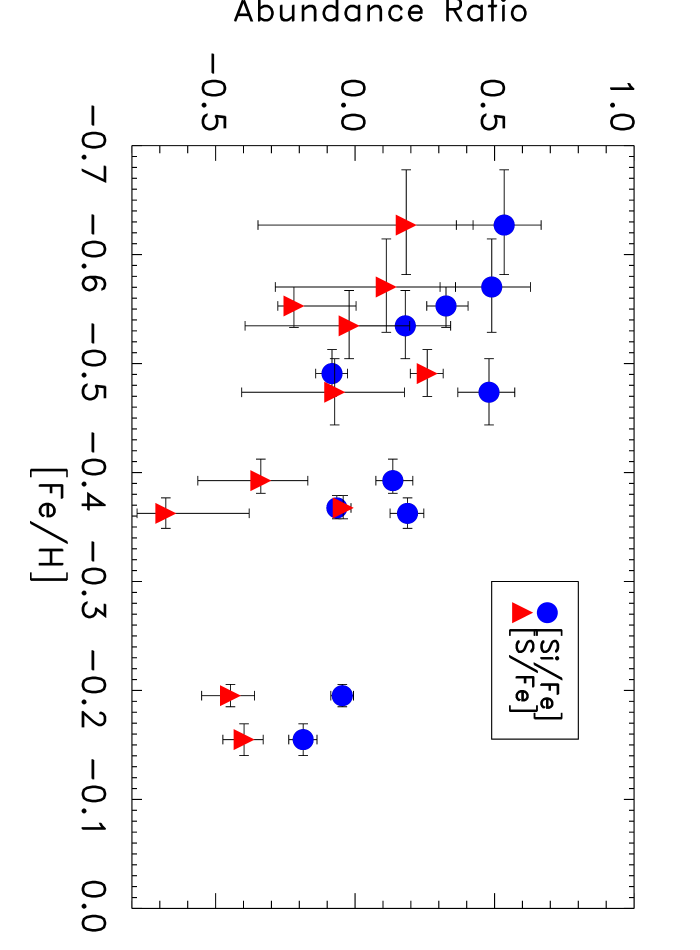
Figure 4.— The silicon and sulfur abundances ratios with respect to iron.

Silicon and sulfur also show disagreement in their trend with temperature — the relative abundance of silicon rises with temperature, and sulfur falls. We find that the silicon abundance rises from $\sim$0.3 solar in cooler clusters to $\sim$0.7 solar in hot clusters, in excellent agreement with the results of Fukazawa et al. (1998).

Calcium and argon are noticeable for their lack of a detectable signal. Both are not detected in the stacked ASCA data, yielding only upper limits over the temperature range from 2–12 keV.

The relative abundances for nickel are measured to be higher than any other element in our study. For clusters hotter than 4 keV, nickel is about 1.2 times the solar value. Lower temperature clusters are too cool to significantly excite the nickel K-$\alpha$ transition, and abundances derived from the Ni L-shell lines are not reliable. The Ni/Fe values are extremely high at about 3 times the solar value, confirming the results of Dupke & White (2000a); Dupke & Arnaud (2001); Dupke & White (2000b).

6. SYSTEMATIC ERRORS

The abundances results in this paper depend upon the measurement of particular spectral lines that are not always very strong. Because of this, a proper understanding of the results must take into account any systematic errors that may bias the results. Of particular concern to this work are systematic errors in the calibration of the effective area, since these often manifest themselves as lines in residual spectra of sources with a smooth continuum. If these residual lines fall at the same energy as the important elemental spectral lines they can have a significant affect on the derived elemental abundances.

The ACC catalog paper discusses general ASCA systematics and our sensitivity to them. In addition, there are several other tests we have undertaken to determine the effect of small line-like systematic errors in the effective area. In order to determine the size of any calibration errors, we have fit spectra from broad band continuum sources and quantified the residuals. We have also used these residuals to correct the cluster spectra, and have compared the derived elemental abundances to those from the uncorrected spectra.

We have used an ASCA observation of Cygnus X-1 (a bright source where the systematic errors dominate the statistical ones) to measure the size of residual lines in fitted spectra of a continuum source. These lines could be due to errors in the instrument calibration and could affect the abundance determinations in clusters. Using a power law + diskline model in XPSEC, we measure the largest residual in the Cyg X-1 spectrum to have an equivalent width of 17 eV at 3.6 eV. Using the Raymond-Smith plasma code to model the equivalent width of elemental X-ray lines, we find that the only element with a small enough equivalent width to be possibly affected by a 17 eV residual is calcium, with an equivalent width of 25 eV for very hot clusters ($>6\,$keV). However, the 17 eV residual lies at the wrong energy to affect calcium (lines at 3.8, 3.9, and 4.1 keV). In addition, the positive residual would serve to increase the measured calcium abundances; our measured calcium abundances are lower than expected. A similar test with the bright continuum source Mkn 421 (with the core emission removed to prevent pileup) shows a maximum residual of 18 eV equivalent width at the 2.11 keV Au edge of the mirror. These results indicate that any line-like calibration errors are not large enough to affect the cluster elemental abundance measurements in this study.

We have also used an ASCA observation of 3C 273 (sequence number 12601000) as a broad band continuum source to check for calibration errors in the response matrices and their effect on the derived cluster elemental abundances. We fit 3C 273 with an absorbed power law model (Figure 5)

Figure 5.— An absorbed power law fit to the ASCA 3C 273 data. The data and model are shown in the top panel for the 4 ASCA detectors, and the ratio of the data to the model is shown in the bottom panel. The lack of any significant residuals indicate that the ASCA effective area calibration is free of any significant line-like systematic errors.

and extracted the ratio residuals to the best fit. We then used these residuals as a correction to the cluster data, and then refit the clusters to find the abundances. The abundances from the corrected data are completely consistent with the abundances from the uncorrected data, further indicating that errors in the effective area calibration do not affect the derived elemental abundances.

We have also investigated the abundances derived using the GIS and SIS detectors separately in order to check the consistency of our results. While the SIS has better spectral resolution, it also suffers from slight CTI and low energy absorption problems that do not affect the GIS. Figure 6

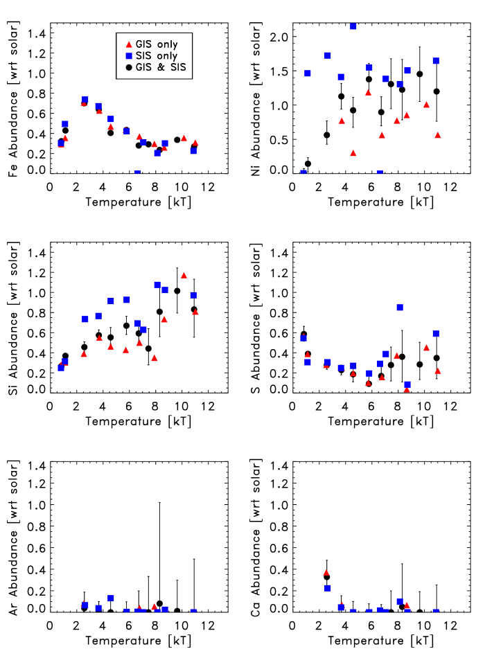
Figure 6.— A comparison of abundance results using the GIS alone, the SIS alone, and the GIS and SIS combined. The GIS and SIS agree well except for nickel and a slight trend in the medium temperature silicon results. The nickel discrepancies are due to the lower effectiveness of the SIS at Ni K, and the SIS silicon measurements suffer from proximity to the detector Si edge. The errorbars for the GIS and SIS alone points are omitted for clarity, but are about a factor of $\sqrt{2}$ larger than those for the combined points.

shows these results. In general, the GIS and SIS abundances match very well for most of the elements. However, nickel and silicon show a systematic trend of slightly higher SIS abundances. The SIS nickel abundances are not as reliable as the GIS abundances because the GIS has more effective area than the SIS at Ni K.

The systematic trend in the medium temperature silicon abundances is more difficult to understand. Fukazawa (1997) showed that the GIS and SIS sulfur and silicon abundances for his cluster sample were well matched. Individual analysis of the bright, medium temperature clusters Abell 496 and Abell 2199 show that the results are indeed real and verify that the SIS gives higher Si abundances than the GIS. Additional fits to the data that allow the SIS gain to vary also do not significantly affect the abundance results. One possible contribution to this problem is that the medium temperature clusters most affected by this trend mostly lie at a redshift such that the Si K-shell lines (1.86 and 2.00 keV) are redshifted very close to the Si edge (1.84 keV) in the detector. These silicon abundances are less reliable because of structure present in the Si edge not well modeled in the instrument response (Mori et al., 2000).

The fit results in the 0.5 and 1.5 keV bins from Tables 3, 4, and 5 show elevated calcium and argon abundances. These very high fit results (1–10 times solar) are not believed to be indicative of the actual cluster abundances because of systematic errors that preferentially affect these low temperature bins. Two sources of systematic error we have identified both become important at low cluster temperatures and affect the modeled spectrum at the higher energies of the Ar and Ca K-shell lines.

The first is background subtraction: because the dominant bremsstrahlung emission is limited to lower energies for the cooler clusters, the cluster flux present at the higher energies of the Ar and Ca K-shell lines becomes comparable to the background. Small errors in the blank sky background can then significantly affect the background-subtracted data, leading to incorrect abundances at higher energies where the relative errors from the background subtraction become large.

Also important at the lower cluster temperatures where the bremsstrahlung emission does not dominate throughout the X-ray spectrum is the contribution from point sources within the individual galaxies. Angelini, Loewenstein, & Mushotzky (2001) and Irwin, Athey, & Bregman (2003) have shown with data from elliptical galaxies that the contribution from X-ray binaries is important and can be characterized with a 7 keV bremsstrahlung model. Since we do not include this component in our cluster fits, we expect that our Ar and Ca abundance for low temperature clusters will be driven upwards in an attempt to try and match the flux actually contributed by the X-ray point sources.

7. COMPARISONS

We believe that X-ray determinations of elemental abundances in galaxy clusters are one of the most accessible means for obtaining useful abundance measurements. While our results are consistent with and significantly expand previous cluster X-ray measurements, they do not always agree with measurements of elemental abundances in other objects.

7.1. Comparison to Other Cluster X-ray Measurements

7.1.1 ASCA Measurements

Measurements of abundances for elements other than iron has historically been difficult because of the low equivalent width of the lines and the limited resolution of X-ray detectors. Aside from a few limited results with crystal spectrometers on Einstein and other satellites, the first chemical abundance measurements of elements other than iron in galaxy clusters was made by Mushotzky et al. (1996) and made use of the high resolution of the CCD cameras onboard ASCA. Their results for 4 moderate temperature (2.5–5.0 keV), very bright clusters show an average Fe abundance of 0.32 solar, 0.65 solar for Si, 0.25 for S, and 1.0 for Ni. All of these results are in agreement with our results for moderate temperature clusters presented in Table 4. Fukazawa et al. (1998) also reported results for the silicon abundance in clusters that used ASCA data. Their results for 40 clusters was in general agreement with the data from Mushotzky et al. (1996), showing a generally constant iron abundance for clusters above 3k̇eV, and also hinted at the silicon trend with temperature presented with more detail here.

Finoguenov, David, & Ponman (2000) and Finoguenov, Arnaud, & David (2001) concentrated on the detection of abundance gradients with ASCA. Their data for Fe and Si at large radii are in agreement with ours. However, they present measurements of S coupled with Ar in order to reduce errors in the S determination. We see that these elements have very different abundances, and can’t compare our data directly to theirs.

7.1.2 XMM Measurements

Further results for the intermediate element abundances in clusters with ASCA were hampered by its moderate resolution, and especially because only a handful of clusters have high enough X-ray flux to allow meaningful measurements. The advent of Chandra and especially XMM have changed this with their higher resolution CCD cameras and much increased effective area. While measurements of argon and calcium are still beset with systematic problems in the XMM response and background subtraction, measurements of silicon and sulfur are largely free of these complications.

The much improved spatial and spectral resolution of XMM allow not only abundance measurements averaged over the whole cluster, but also spatially resolved ones. While our measurements in clusters are overall spatial averages, the measurements with XMM are usually spatially resolved and give information on abundance gradients within clusters. While this information is important and sheds valuable light on the enrichment mechanisms in clusters, we will limit our comparisons to overall abundances measured with XMM, or with abundances in the more voluminous outer regions of clusters with spatially resolved abundances.

The many XMM papers on M87 (Böhringer et al., 2001; Molendi & Gastaldello, 2001; Gastaldello & Molendi, 2002; Matsushita, Finoguenov, & Böhringer, 2003) all find a significant abundance gradient in the center of the cluster. In the very center, Molendi & Gastaldello (2001) find generally higher abundances than in the outer regions, with the iron abundance at about 0.6 the solar value. They find silicon to be 1.0 in the same region, giving [Si/Fe] only slightly lower than our results for a similar temperature cluster. However, sulfur is about 1.1 solar, overly abundant with respect to iron than in our results. The discrepancies between some of our results for 2.5 keV clusters and the XMM M87 results are tempered by the fact that earlier ASCA results for M87 (Matsumoto et al., 1996; Guainazzi & Molendi, 1999) are similar to the XMM results, and by the fact that the M87 data is for only one cluster, while our ASCA results are for an average of several clusters at the same temperature.

Tamura et al. (2001) find sulfur and silicon to have similar abundances in the center of A496 with RGS data from XMM, slightly different than our results that show silicon slightly higher than sulfur by a factor of about 1.5. Unfortunately, the M87 data concentrates on the cluster core, and the A496 data is taken with the RGS, which also is limited to the centers of bright clusters. This bias towards the very centers of clusters makes a comparison with our average cluster abundances difficult.

Finoguenov et al. (2002) also look at XMM data for M87, but focus their paper on a discussion of the supernovae enrichment needed to account for the observed abundances. Their data leads them to conclude, as we do, that the standard yields of the canonical SN Ia and SN II models are not sufficient to explain the pattern of abundances observed. Their solution calls for an additional source of metals from a new class of type I supernovae. This scenario does not fit our data well; specifically, it leads to an overproduction of sulfur, argon and calcium, with not enough silicon produced to match our observations. Finoguenov et al. (2002) focus on the inner the inner 70 kpc region of M87 because of the cluster’s proximity. Their results in this region are where the influence of the galaxy’s stellar population and associated SNIa are most keenly apparent. Even at the outer parts of this region, the abundances show signs of a transition to a more typical cluster pattern. This inner region contributes a small fraction of the emission measure of most systems in our ACC sample, and makes comparisons difficult since we sample different areas of the cluster.

7.2. Comparison to Measurements in Different Types of Objects

7.2.1 The Thin Disk

The standard solar elemental composition is based on measurements taken of the sun, which resides in the thin disk of the galaxy. Our cluster results show significant differences with stellar data from the thin disk. Figure 7

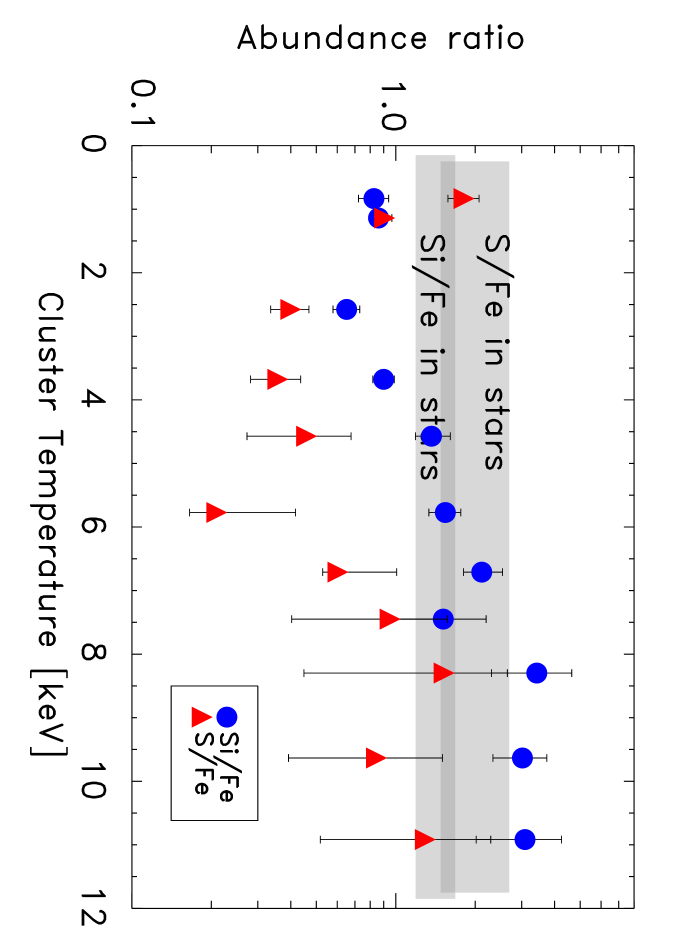
Figure 7.— The silicon and sulfur abundances as a function of temperature, compared to their abundance in stars. The upper grey bar is the S/Fe data from Timmes, Woosley, & Weaver (1995), and the overlapping lower grey bar is the Si/Fe data from the same source.

shows silicon and sulfur abundance ratios in clusters compared with data from Timmes, Woosley, & Weaver (1995). The stellar data is overplotted on the cluster points as grey bars. The [Si/Fe] cluster data overlaps with the stellar data, but has a much greater range. The [S/Fe] cluster data lies almost totally below the stellar data. The largest discrepancy is between the cluster and stellar nickel abundance ratios; clusters are higher than the stellar data of 0.1 by 0.5 dex. This very high value for [Ni/Fe] is not seen in stars at any metallicity.

7.2.2 The Thick Disk

The majority of the stellar mass in clusters resides in elliptical galaxies and the bulges and halos of spirals (Bell, McIntosh, Katz, & Weinberg, 2003). Prochaska et al. (2000) find that the abundance patterns of the thick disk are in excellent agreement with those in the bulge, suggesting that the two formed from the same reservoir of gas. If this is true, and if the majority of the enriched gas in the ICM originated in these numerically dominant stellar populations, then we would expect that the abundance pattern in the ICM is in good agreement with that in the thick disk of the Milky Way. However, reality is more complicated. While Prochaska et al. (2000) find that the thick disk has enhanced abundances for the $\alpha$ elements compared to the thin disk and solar neighborhood, they also find [Ni/Fe] in the thick disk is similar to its solar value. Additionally, the calcium abundance ratio is found to be super solar ([Ca/Fe] = 0.2), and sulfur is more enhanced with respect to iron in the thick disk than in clusters. Also, the recent work of Pompeia, Barbuy, & Grenon (2003) shows a [Si/Fe] value of nearly 0.0, much lower than what we observe here.

7.2.3 H II Regions and Planetary Nebulae

Comparison of our cluster results with H II regions or planetary nebulae is difficult because of the strong effects of dust and non-LTE conditions on abundance measurements of elements like iron and silicon (Peimbert, Carigi, & Peimbert, 2001; Stasinska, 2002). C, N, and O are more readily observed in these objects, but are not observed with ASCA.

7.2.4 Damped Ly-$\alpha$ Absorbers

Prochaska & Wolfe (2002) show abundance measurements from a large database of damped Ly-$\alpha$ (DLA) observations. Their results are for the redshift range $1.5<z<3.5$ and indicate that there is already significant $\alpha$ element enhancement at high redshifts. This conclusion is consistent with that reached by Mushotzky et al. (1996) in an analysis of high redshift clusters. The [Fe/H] value observed by Prochaska & Wolfe of -1.6 is constant over a wide range of redshift, indicating that the enrichment was at earlier times. This value is much lower than our value of [Fe/H] = -0.5 (for our higher temperature bins where the iron abundance is fairly constant), showing the importance of supernovae enrichment in the ICM. Their average [Si/Fe] value of 0.35 agrees with our results for moderate temperature clusters, and their spread of [Si/Fe] measurements from 0.0 to 0.5 is well matched with ours. Their [Si/Fe] values are also constant over a wide redshift range, further supporting early enrichment. However, their results for sulfur differ from ours in that they show more enrichment with respect to iron ([S/Fe] $\sim$ 0.4) than we do. This suggests that later enrichment by supernovae into the ICM had a reduced role for sulfur in comparison to the other elements. Nickel is also different in these systems than in clusters, with [Ni/Fe] of only 0.07; much different than our very high value of $\sim$0.5. While Prochaska & Wolfe (2002) have some results for argon, they are widely scattered and not easily interpreted. The differences with the cluster measurements of S and Ni indicate that the stellar population that enriched these systems is probably not the origin of the metals in the ICM.

7.2.5 Lyman Break Galaxies

Pettini et al. (2002) present detailed observations of a lensed Lyman break galaxy at $z=2.7$. Their results also indicate that significant metal enrichment have already taken place at high redshift. Their results for O, Mg, Si, S, and P are all at about 0.4 the solar value, showing the results of fast supernovae processing. However, the iron peak elements are not as enriched, with the values of Mn, Fe, and Ni at only 1/3 solar. The interpretation is that this galaxy has been caught in the middle of turning its gas into stars, and that while enrichment from SN II has occurred, not enough time has passed to allow significant enrichment from the iron peak producing SN Ia. The overall metallicity of [Fe/H] = -1.2 is closer to our observed cluster value than the measurements from the DLAs are. However, the abundance ratios in this object are also sufficiently different than in clusters to indicate that the stellar population that enriched the Lyman break galaxies is also probably not the source of the metals in the ICM.

7.2.6 The Ly-$\alpha$ Forest

While it is possible to probe the metallicity history of the universe as a function of redshift (Songaila, 2001; Songaila & Cowie, 2002), the difficulty inherent in measuring lines from many different elements in the Ly-$\alpha$ forest has made abundance measurements of most elements besides Fe, C, N, and Si unavailable. Ly-$\alpha$ forest measurements show metallicities of [Fe/H] ranging from -2.65 at a redshift of 5.3 to -1.25 at redshift 3.8. All of these are almost two orders of magnitude lower than our measurements.

8. SUPERNOVAE TYPE DECOMPOSITION

With the results of § 5 for the abundance of the intermediate elements in clusters, it is possible to try to constrain the mix of supernovae types that have enriched the ICM. In § 8.1, we check to see how well the yields from the standard SN Ia and SN II models can reproduce the cluster observations. We find that other sources of metals are necessary. Then we comment on the expected cluster abundances derived using some of the standard models in the literature. In § 8.3, we investigate different SN models that produce intermediate elements with the abundance ratios necessary for reconciling the models with the observations.

8.1. SN Fraction Analysis using Canonical SN Ia and SN II Models

We use the yields of the revised W7 model (Nomoto et al., 1997b) for SN Ia and the TNH-40 yields (Nomoto et al., 1997a) (mass-averaged by integrating across the IMF to an upper limit of 40 solar masses) for SN II (shown in Figure 8)

Figure 8.— The Type Ia and Type II supernovae yields. The horizontal axis is atomic number — O is 8, Fe 26, Si 14, S 16, Ni 28. The yields are in solar masses per supernova. Iron comes mostly from SN Ia  and nickel even more so. Si, S, Ar, and Ca are a mix of SN II and SN Ia  but with a majority SN II contribution. The SN Ia data comes from the W7 model, and the SN II data is from the IMF mass-averaged TNH-40 model.

as our basis. Each model includes the amount of each of the intermediate elements produced in a supernova of that type.

We used the data from the models to produce a table with the yields and abundance ratios for 100 different mixtures of SN Ia and SN II ranging from pure SN Ia enrichment to pure SN II enrichment. We then compare our two best-measured cluster abundance ratios (Si/Fe and S/Fe) with the model ratios in order to arrive at a SN type fraction. The results are plotted in Figure 9

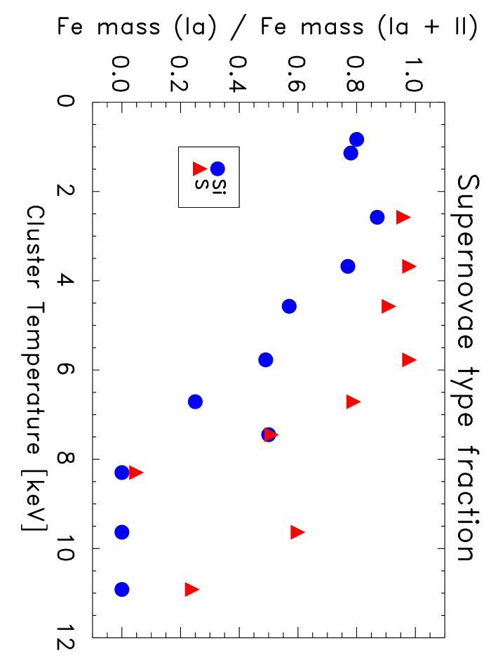
Figure 9.— The supernovae-type ratio derived from the silicon and sulfur abundances. The SN Ia yields of the W7 model (Nomoto et al., 1997b) and the SN II yields of the IMF mass-averaged TNH-40 (Nomoto et al., 1997a) model were used to compute the Si/Fe and S/Fe abundance ratios for 100 mixtures ranging from pure SN Ia enrichment to pure SN II enrichment. The measured data was compared to the model output in order to determine the relative ratio of SN Ia and SN II. A value of 1 on the plot indicates enrichment by solely SN Ia  while a value of 0 indicates enrichment solely by SN II.

and show the SN type fraction derived from both Si/Fe and S/Fe as a function of cluster temperature.

The difficulty of calculating SN yields leads to acknowledged uncertainties for some of the elements of about a factor of two (Gibson, Loewenstein, & Mushotzky, 1997). In order to investigate the effects of different SN models on the derived SN fraction, we have compared the SN fractions derived from several different SN models in Figure 10.

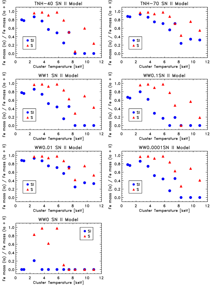
Figure 10.— The supernovae-type ratio derived from the silicon and sulfur abundances, comparing the results from many different SN II models. This figure is similar to Figure 9, but shows that many different SN II models all have difficulty producing a consistent type fraction from the silicon and sulfur data. Also, the trend of cooler clusters predominantly enriched by type SN Ia products and hotter clusters enriched by SN II products does not depend on the SN II model used. Again, a value of 1 on the plot indicates enrichment by solely SN Ia  while a value of 0 indicates enrichment solely by SN II.

Each SN fraction determination uses the W7 SN Ia model as revised in Nomoto et al. (1997b), but uses a different SN II model. The result of this comparison indicates that different SN II models can change the average value for the derived SN fraction, but does not change the fact that none of the seven SN II models results in a consistent SN fraction from both the cluster Si/Fe and S/Fe data.

The results we have found for the cluster intermediate element abundances do not fit the standard model where most of the elements are produced in a simple mix of standard SN Ia and SN II events. The observed silicon abundance is too high with respect to iron, and the observed sulfur abundance too low. Calcium and argon are also too low. The SN type fractions derived from the two abundance ratios are not consistent with each other, and change dramatically as a function of cluster temperature. These results indicate that a unique, consistent decomposition of the ICM enrichment into SN Ia and SN II contributions is not possible.

Faced with these inconsistencies, new models must be examined that can better explain our results. Some possibilities are included in the following section.

8.2. Expected Abundances from Standard SN Models

Table 7Observed and Model Abundances

Element	ASCA	SN II	SN Ia	SN II+SN Ia	+SN IIx	+SN IIx	+SN IIx
Si	0.6–0.8	0.34	0.095	0.40	0.70	0.7	0.70
S	0.1–0.4	0.20	0.090	0.30	0.40	0.3	0.40
Ar	0.0–0.2	0.17	0.075	0.25	0.30	0.2	0.30
Ca	0.0–0.2	0.19	0.090	0.30	0.35	0.3	0.35
Fe	0.4	0.14	0.260	0.40	0.40	0.4	0.40
Ni	0.8–1.5	0.16	0.850	1.00	1.00	1.0	1.00

Note. — Abundances are given with respect to the solar values in Table 3, column 3.

There are many different supernovae yield computations in the scientific literature. For SN II, there are variations in the progenitor masses, metallicities and internal structure; in explosion energy and placement of the mass cut; and in adopted nuclear reaction rates. For SN Ia, parameters include the central white dwarf progenitor density and burning front propagation speed. Initially, we consider the standard W7 deflagration SN Ia model and Salpeter-IMF-averaged SN II yields from Nomoto et al. (1997b). In all cases, a combination of SN Ia and SN II yields is necessary to match the observed results.

About 0.02 SN II events per current solar mass of stars will occur if most of the stars in cluster galaxies form over an interval much shorter than the age of the universe (indicated by the predominance of early-type galaxies in clusters) and if star formation proceeds with a standard IMF (Kroupa, 2002). This calculation takes the mass lost to winds and remnants into account and assumes the SN II progenitors are stars with original mass $>$ 8 M_☉. Column 2 of Table 7 shows the observational range we aim to explain, Column 3 of Table 7 shows the model abundances from ICM enrichment by SN II (for the gas-to-star mass ratio of 10 that is typical of a rich cluster).

If the assumption is made that SN Ia provide the remainder of the iron (The enrichment levels due solely to SN Ia enrichment are in column 4 of Table 7), then the total expected abundances (SN II + SN Ia) are as shown in column 5 of Table 7. The number of SN Ia required corresponds to an average of 1.8 SNU over $10^{10}$ years for a typical ratio of ICM mass to stellar blue light of 40, significantly higher than the estimated optical rate at $z=0$ (Cappellaro et al., 1997). This combination of SN II and SN Ia accounts for the observed abundances of nickel and sulfur (compare columns 2 and 5 of Table 7). However, only about half of the observed silicon is accounted for and calcium and argon are slightly overproduced. Different models must be investigated to make up this significant shortfall. The most variation in SN yields is in SN II models, and we explore some of these alternatives below.

Unfortunately, many SN II models, in particular those of Woosley & Weaver (1995) and Rauscher, Heger, Hoffman, & Woosley (2002), generally derive higher yields of sulfur, argon and calcium that exacerbate the conflict between theory and observations. In addition, SN II iron yields are uncertain by at least a factor of two (Gibson, Loewenstein, & Mushotzky, 1997) because of their sensitivity to the assumed mass cut. If one arbitrarily and exclusively increases the SN II contribution to the iron yield by a factor of two, then the SN Ia contribution to sulfur, argon and calcium goes down by a factor of two and is in marginal agreement with the observations. Unfortunately, this scenario increases the silicon deficit and the nickel abundance falls to the unacceptably low value of about half solar.

Models that explicitly synthesize more iron (e.g., those of Woosley & Weaver (1995) with enhanced explosion energy) also generally produce more sulfur, argon and calcium that enhances the problem with those elements. However, the Woosley & Weaver (1995) enhanced energy models having zero metallicity progenitors have a very different nucleosynthetic profile — the production of iron and nickel averaged over the IMF is doubled without an increase in sulfur, argon and calcium. Unfortunately, silicon and nickel remain underproduced by a factor of two if these SN II yields are adopted.

Other variations on the SN II yields also fail to explain the low ratio of sulfur, argon and calcium to silicon. Neither adopting delayed detonation SN Ia models (Finoguenov et al., 2002) nor increasing the silicon abundance by assuming a flat IMF (Loewenstein & Mushotzky, 1996) solves the problem. Finoguenov et al. (2002) explain the abundance pattern and its radial variation in M87 by proposing (1) a radially increasing SNII/SNIa ratio, (2) high Si and S yields from SNIa (favoring delayed detonation models) and an ad hoc reduction in SNII S yields, and (3) a radial variation in SNIa yields (corresponding to delayed detonation models with different deflagration-to-detonation transition densities). While this scenario appears promising with regard to the galaxy-dominated inner regions of rich clusters and, perhaps groups, there are difficulties – as Finoguenov et al. (2002) acknowledge – in explaining the pattern in the large scale abundances of high-temperature clusters.

One possible solution is to assume a flat IMF to boost SN II silicon production (and account for at least half of the iron), combined with ad hoc reductions in sulfur, argon and calcium yields by a factor of two. An increase in the SN II nickel yields (uncertain by a factor of two because of mass cut and core neutron excess uncertainties, Nakamura et al. 1999) would also have to be instated to account for the lowered nickel from the reduced SN Ia output. On the other hand, if a standard IMF is maintained, then less significant decreases in SN II production of sulfur, argon and calcium are needed. For this case, the silicon deficit would have to be made up by another mechanism; enhanced hydrostatic production of silicon or a suppressed efficiency of silicon burning are possibilities.

8.3. Alternate Enrichment Scenarios

If the observed cluster iron abundance and stellar elemental abundances are used to set the contribution from supernovae, then the theoretical yields will meet or slightly exceed the ASCA abundance observations for argon and calcium while silicon itself will be significantly underproduced by a factor of $\sim$2. If we accept the standard SN II enrichment given in column 3 of Table 7, then we must have an additional nucleosynthetic source that produces substantial silicon, but little or no sulfur, argon, or calcium. Some possibilities exist in the literature, and we explore some of these scenarios below. We have chosen single mass SN II models that can selectively enhance silicon, and collectively call these models “SN IIx” to distinguish then from the canonical SN II models. For the models presented below, we calculate the number of SN IIx events necessary to produce the observed amounts of iron and silicon that are not produced by regular SN II.

8.3.1 Very Massive Stars

Thielemann, Nomoto, & Hashimoto (1996) have calculated the yields for a 70 M_☉ progenitor with solar metallicity. The abundance ratios in the ejecta with respect to silicon are: 0.4, 0.28, 0.26, 0.048, and 0.12 relative to solar for S, Ar, Ca, Fe, and Ni. With these results, the observational overabundance of silicon can be accounted for with $\sim 2\times 10^{-4}$ SN IIx per solar mass in the ICM. This rate will provide the extra silicon necessary, is only about 10% of the total number of SN II expected by integrating a normal IMF, and only produces minor perturbations in the other elements. The abundances expected from the combination of SN Ia, canonical SN II, and SN IIx from very massive progenitors is given in column 6 of Table 7.

8.3.2 Massive, Metal-poor Stars

Very small amounts of the elements heavier than silicon are produced in the high mass ($>$ 25 M_☉), low-metallicity (0.01, 0.1 solar) models of Woosley & Weaver (1995). These yields give less than 10% of the solar ratios (with respect to silicon) for elements heavier than silicon. Hence, silicon abundances can be increased without causing the other elements to exceed their observed values. In order to produce the observed abundances, about $5.7\times 10^{-4}$ SN IIx per solar mass in the ICM are necessary, assuming progenitors of 30–40 M_☉ with 0.01 solar abundance and an IMF that goes as $M^{-1}$. The abundances expected from the combination of SN Ia, canonical SN II, and SN IIx from massive, metal-poor progenitors is given in column 7 of Table 7.

8.3.3 Population III Stars

The ejecta of supernovae preceded by very massive, zero metallicity progenitor stars (Pop III stars) have a substantially different composition than standard SN II ejecta (e.g., Heger & Woosley (2002)). If the Pop III mass function is dominated by the low mass (He cores $<80$ M_☉) models of Heger & Woosley (2002), then the relative Si overabundance from observations can be explained. If higher core masses are used, the silicon overabundances are not as well explained, but more modest underabundances are found for sulfur, argon, and calcium. For example, about $2.3\times 10^{-5}$ SN IIx events per solar mass in the ICM from progenitors with 70 M_☉ He cores matches our observed abundances and produce the abundances given in column 8 of Table 7.

Figure 11

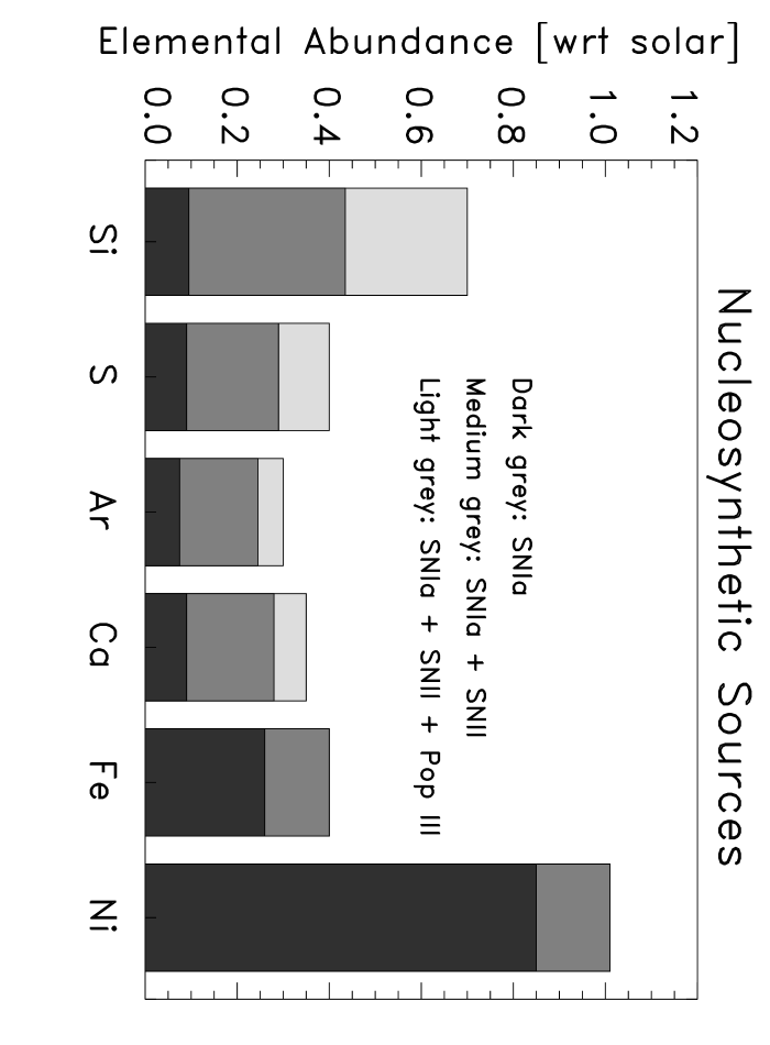
Figure 11.— A decomposition of the intermediate element abundances into their nucleosynthetic origins based on Table 7. The lowest band in each bar is the contribution from SN Ia, the middle band adds the yields from the canonical SN II, and the top band includes the contribution from an early population of high mass, low metallicity Pop III supernovae progenitors. Iron and nickel both are dominated by SN Ia products, with no contribution by SN IIx from Pop III progenitors.

is based on Table 7 and shows graphically what proportion of each element’s abundance comes from SN Ia, SN II, and SN IIx. The three different SN IIx models all produce similar results, and provide the silicon necessary to match the observational overabundance without unduly exacerbating the low observed abundances of sulfur, argon and calcium.

8.4. Discussion

The anomalous abundance patterns found here in galaxy clusters are unique. The relative simplicity and uncomplicated nature of the X-ray emission from clusters and their role as a repository for all the enriched gas produced by supernovae makes them important objects for understanding the production and evolution of metals in the universe.

However, no combination of SN Ia and SN II products using current theoretical yields can produce the abundances observed with ASCA. Manipulating the standard models by changing the IMF or appealing to different physical models such as delayed detonation can help mitigate only some of the inconsistencies between models and observations. A new source of metals is needed in order satisfactorily explain the cluster abundances. The low ratios of S/Si, Ar/Si and Ca/Si are indicative of a fundamentally different mode of heavy metal enrichment. We have identified three different SN models that can produce these metals in the correct proportions and have calculated the number of events necessary to match the observations when combined with metals produced in ordinary SN Ia and SN II. These models all have in common very massive, metal poor progenitor stars.

It is natural to associate these with the earliest generation of (Pop III) stars. This primordial population must have existed, and its distinct characteristics are well matched to those required to explain the ICM abundance anomalies: zero metallicity, and a top-heavy IMF that has an important contribution from very massive stars (Bromm, Coppi, & Larson, 1999; Abel, Bryan, & Norman, 2000). Enhanced explosion energies are indicated, and nucleosynthetic production is high with an abundance pattern quite distinct from other SN II (Heger & Woosley, 2002).

Loewenstein (2001) proposed hypernovae associated with Pop III as a means of enhancing silicon relative to oxygen in the ICM, and inferred a hypernovae rate of the same order as the SN IIx from Pop III stars derived here. The precise required number is subject to assumed values of the ICM/stellar ratio, the IMF and SN II yields for Pop II stars, and the IMF and SN IIx yields for Pop III stars, but is in the range of 10–30 times larger than the average value ($\Omega_{III}\sim 4\times 10^{-6}$) predicted in the semi-analytic models of Ostriker & Gnedin (1996). This could be the result of enhanced primordial star formation in these extremely overdense environments. Evidence also exists for more nearly solar abundance ratios in less massive clusters (Finoguenov et al., 2002).

Both observations and theory suggest the idea that a large population of massive, metal-poor Pop III stars was present at very high redshift and constituted the first generation of stars. The heavy metal products from this first generation would have been formed at the same time as the first galaxies or even before, and would now be widely dispersed in the ICM. Galaxy clusters serve as the largest repositories of both enriched gas from cluster galaxies and of gas expelled by the earliest generations of stars and then accreted onto clusters. A combination of X-ray observations well matched to observing metal abundances in clusters and the importance of galaxy clusters as large retainers of Pop III enriched gas make these observations one of the best views onto the earliest generations of stars in the universe.

9. SUMMARY

We have presented intermediate element abundances for galaxy clusters based on ASCA observations. Our measurements of the iron and silicon abundances agree with the past ASCA results of Fukazawa (1997) and Mushotzky et al. (1996), but achieve much higher precision and extend the temperature range from 0.5–12 keV. The measurements of the individual element abundances show some surprising new results: silicon and sulfur do not track each other as a function of temperature in clusters, and argon and calcium have much lower abundances than expected.

These results show that the $\alpha$-elements do not behave homogeneously as a single group. The unexpected abundance trends with temperature probably indicate that different enrichment mechanisms are important in clusters with different masses. The wide scatter in $\alpha$-element abundances at a single temperature could indicate that SN models need some fine tuning of the individual element yields, or that a different population of SN needs to be considered as important to metal enrichment in clusters.

We have also attempted to use our measured abundances to constrain the SN types that caused the metal enrichment in clusters. A first attempt to split the metal content into contributions from canonical SN Ia and SN II led to inconsistent results with both the individual elemental abundances and with the abundance ratios of our most well measured elements. An investigation of different SN models also could not lead to a scenario consistent with the measured data, and we deduce that no combination of SN Ia and SN II fits the data. Another source of metals is needed.

This extra source of metals must be able to produce enough silicon to match the measurements, but not so much sulfur, argon, or calcium to exceed them. An investigation of SN models in the literature led to three separate models that could fulfill these requirements. All three models were similar, and had as progenitor stars massive and/or metal poor stars. The combination of canonical SN Ia and SN II with one of the new models does a much better job of matching the observations. These sorts of massive, metal poor progenitor stars are exactly the stars that are supposed to make up the very early Population III stars. The conjunction of our required extra source of metals with SN from population III-like progenitors supports the idea that a significant amount of metal enrichment was from the very earliest stars.

Clusters are a unique environment for elemental abundance measurements because they retain all the metals produced in them. The relatively uncomplicated physical environment in clusters also allows well-understood abundance measurements. Future abundance analyses using a large sample of XMM data will allow an even better understanding of the SN types and enrichment mechanisms important in galaxy clusters.

References

- Abel, Bryan, & Norman (2000) Abel, T., Bryan, G. L., & Norman, M. L. 2000, ApJ, 540, 39
- Allende Prieto, Lambert, & Asplund (2001) Allende Prieto, C., Lambert, D. L., & Asplund, M. 2001, ApJ, 556, L63
- Anders & Grevesse (1989) Anders, E. & Grevesse, N. 1989, Geochim. Cosmochim. Acta, 53, 197
- Angelini, Loewenstein, & Mushotzky (2001) Angelini, L., Loewenstein, M., & Mushotzky, R. F. 2001, ApJ, 557, L35
- Arnaud et al. (2001) Arnaud, M., Neumann, D. M., Aghanim, N., Gastaud, R., Majerowicz, S., & Hughes, J. P. 2001, A&A, 365, L80
- Arnaud et al. (1992) Arnaud, M., Rothenflug, R., Boulade, O., Vigroux, L., & Vangioni-Flam, E. 1992, A&A, 254, 49
- Becker et al. (1979) Becker, R. H., Smith, B. W., White, N. E., Holt, S. S., Boldt, E. A., Mushotzky, R. F., & Serlemitsos, P. J. 1979, ApJ, 234, L73
- Bell, McIntosh, Katz, & Weinberg (2003) Bell, E. F., McIntosh, D. H., Katz, N., & Weinberg, M. D. 2003, ArXiv Astrophysics e-prints, 2543
- Böhringer et al. (2001) Böhringer, H. et al. 2001, A&A, 365, L181
- Bromm, Coppi, & Larson (1999) Bromm, V., Coppi, P. S., & Larson, R. B. 1999, ApJ, 527, L5
- Cappellaro et al. (1997) Cappellaro, E., Turatto, M., Tsvetkov, D. Y., Bartunov, O. S., Pollas, C., Evans, R., & Hamuy, M. 1997, A&A, 322, 431
- DeGrandi (2003) DeGrandi, S. 2003 in proceedings of the Ringberg Cluster Conference
- Dupke & Arnaud (2001) Dupke, R. A. & Arnaud, K. A. 2001, ApJ, 548, 141
- Dupke & White (2000a) Dupke, R. A. & White, R. E. 2000a, ApJ, 528, 139
- Dupke & White (2000b) Dupke, R. A. & White, R. E. 2000b, ApJ, 537, 123
- Finoguenov, Arnaud, & David (2001) Finoguenov, A., Arnaud, M., & David, L. P. 2001, ApJ, 555, 191