Digital Deblurring of CMB Maps II:
Asymmetric Point Spread Function

In this second paper in a series dedicated to developing efficient numerical techniques for the deblurring Cosmic Microwave Background (CMB) maps, we consider the case of asymmetric point spread functions (PSF). Although conceptually this problem is not different from the symmetric case, there are important differences from the computational point of view because it is no longer possible to use some of the efficient numerical techniques that work with symmetric PSFs. We present procedures that permit the use of efficient techniques even when this condition is not met. In particular, two methods are considered: a procedure based on a Kronecker approximation technique that can be implemented with the numerical methods used with symmetric PSFs but that has the limitation of requiring only mildly asymmetric PSFs. The second is a variant of the classic Tikhonov technique that works even with very asymmetric PSFs but that requires discarding the edges of the maps. We provide details for efficient implementations of the algorithms. Their performance is tested on simulated CMB maps.

1 Introduction

In the first paper in the series Vio et al. (2003) (VNT) have stressed the advantage of deblurring small patches of the sky in cosmic microwave background (CMB) studies: first, it helps to recover high frequencies smoothed out by the instrument’s PSF. Second, a better understanding of sky emissions, from foregrounds in particular, is achieved if multifrequency sky maps are compared on a common resolution. Third, some map-based component separation algorithms, such as independent component analysis (Baccigalupi et al. 2000; Maino et al. 2002), require input maps with similar level of degradation. Furthermore, although the aim of satellite missions such as Planck and MAP is to obtain full sky maps of the CMB, the strength of the CMB over other backgrounds or contaminating sources will vary over the sky. As a result, even a successful separation of the components contributing to the microwave radiation will provide results of inhomogeneos quality. Therefore, even if some characteristics of CMB are estimated on full sky maps, it will be important to check these results on smaller sky patches where CMB largely dominates the other components (i.e., no component separation is necessary as, e.g., at high Galactic latitude and at high observing frequency) and data are free from instrumental and/or observational problems. We stress that a gain in resolution is always possible also when maps of different resolutions are composed together, for example, through the method described in Tegmark (1999).

VNT suggested a deblurring approach based on Tikhonov regularization whose computational cost is comparable to that of classic frequency domain methods but that leads to more reliable and stable deblurring estimates. These new efficient implementations make the Tikhonov technique a promising tool for deblurring CMB maps. The main limitation of the method is the requirement of symmetric PSFs, which prevents its application in the general experimental context with no restriction on the form of the PSF. This point is especially important in CMB experiments where an asymmetric PSF can alter the results of the analyses, for example, by distorting the estimated angular power spectrum or by altering the measure of the degree of nonGaussianity of the maps. Since some experimental situations are not well controlled, one should develop algorithms that can cope with the worst possible scenario; it is thus important to develop deblurring methods for asymmetric PSFs.

In Sect. 2 we formalize the problem and propose two solutions in Sects. 3 and 4: the first one is a very efficient method but requires only mildly asymmetric PSFs, whereas the second, although less efficient, is not limited by the particular form of the observing beam. A modification of the second method is considered in Sect. 5. The results of numerical simulations to test the performance of the different methods are presented in Sect. 6. In Sect. 7 we close with final comments and conclusions.

2 Formalization of the problem

We make use of the same formalism adopted in VNT. When a two-dimensional object $f(\xi,\eta)$ is observed through an optical invariant (linear) system, it is seen as an image $g(x,y)$,

$$g(x,y)=\int\limits_{-\infty}^{+\infty}\int\limits_{-\infty}^{+\infty}h(x-\xi,y-\eta)f(\xi,\eta)\leavevmode\nobreak\ d\xi\leavevmode\nobreak\ d\eta,$$ (1)

where the space-invariant point-spread function (PSF) $h(x-\xi,y-\eta)$ represents the blurring action of the optical instrument. This model is only theoretical, in practical applications we only have discrete noisy observations of the image $g(x,y)$, which we model as a discrete linear system

$$\boldsymbol{g}=\boldsymbol{H}\boldsymbol{f}+\boldsymbol{z},$$ (2)

where: $\boldsymbol{g}={\rm vec}(\boldsymbol{G})$ and $\boldsymbol{f}={\rm vec}(\boldsymbol{F})$ are one-dimensional column arrays containing, respectively, the observed image $\boldsymbol{G}$ and the true images $\boldsymbol{F}$ in stacked order, $\boldsymbol{z}$ is an array containing the noise contribution (assumed to be additive), and $\boldsymbol{H}$ is a matrix that represents the discretized blurring operator.

There are two problems in obtaining an estimate of $\boldsymbol{f}$ from $\boldsymbol{g}$: the size of the matrix $\boldsymbol{H}$, which is large even for moderate size images, and the very ill-posed nature of the problem. VNT proposed a deblurring method for CMB applications that is efficient and numerically stable; it is a Tikhonov regularization approach where the estimate $\boldsymbol{f}_{\lambda}$ of $\boldsymbol{f}$ is defined as

$$\boldsymbol{f}_{\lambda}={\rm argmin}\left(\,\|\,\boldsymbol{H}\boldsymbol{f}-\boldsymbol{g}\,\|_{2}^{2}+\lambda^{2}\|\,\boldsymbol{L}\boldsymbol{f}\,\|_{2}^{2}\,\right),$$ (3)

with $\lambda$ a scalar regularization parameter. $\boldsymbol{L}$ is often the identity matrix or a discrete derivative operator of some order.

An additional problem is the selection of boundary conditions (BC) to account for data outside the field of view. VNT found that better deblurring estimates of CMB maps were obtained with reflexive BC. This choice leads to reliable and stable regularization parameter estimates, and helps suppress spurious features such as Gibbs oscillations. Periodic and zero BC impose edge discontinuities which bias the image Fourier coefficients and affect the reliability of the regularization parameter estimates obtained through generalized cross-validation (GCV).

On the other hand, efficient implementations of Tikhonov deblurring with reflexive BC require symmetric PSF (although not necessarily separable), i.e., $h(x,y)=h(-x,y)=h(x,-y)=h(-x,-y)$. Since the PSF may be asymmetric in some practical applications (there are indications that this may be the case for PLANCK’s optics), we consider efficient implementations of Tikhonov deblurring that can be used in this case. In particular, in Sect. 3 we consider a very efficient method based on reflexive BC that, however, works only when the PSF is slightly asymmetric. In Sect. 4 a less efficient method, based on periodic BC, is presented; its performance is not sensitive to the specific form of the PSF. For this last case we have to modify the traditional GCV to provide regularization parameter estimates in the presence of edge discontinuities.

3 Kronecker approximation

One possible alternative when the PSF is not symmetric is to determine if the PSF is at least separable; that is,

$$h(x,y)=h_{x}(x)h_{y}(y)\,.$$ (4)

If this is the case, then the corresponding $n^{2}\times n^{2}$ matrix $\boldsymbol{H}$ can be written as

$$\boldsymbol{H}=\boldsymbol{A}\otimes\boldsymbol{B}\,,$$ (5)

where $\boldsymbol{A}$ and $\boldsymbol{B}$ are $n\times n$ matrices, and $\otimes$ is used to denote a Kronecker product

$$\boldsymbol{A}\otimes\boldsymbol{B}=\left(\begin{array}[]{cccc}a_{11}\boldsymbol{B}&a_{12}\boldsymbol{B}&\cdots&a_{1n}\boldsymbol{B}\\ a_{21}\boldsymbol{B}&a_{22}\boldsymbol{B}&\cdots&a_{2n}\boldsymbol{B}\\ \vdots&\vdots&&\vdots\\ a_{n1}\boldsymbol{B}&a_{n2}\boldsymbol{B}&\cdots&a_{nn}\boldsymbol{B}\end{array}\right)\,.$$

For such a structured matrix, algorithms can be implemented efficiently. The cost is $O(n^{3})$, which is slightly more than the $O(n^{2}\log n)$ required of transform-based methods, but is still very reasonable for large images; see VNT for further details. Therefore, we should exploit this structure if we can recognize that the blur is separable.

The key point that permits the development of an efficient algorithm is that if $\boldsymbol{P}$ is an $n\times n$ array of pixels representing the observed PSF and the blur is separable, then $\boldsymbol{P}$ is a rank-one matrix; that is, $\boldsymbol{P}$ can be written as an outer product

$$\boldsymbol{P}=\boldsymbol{a}\boldsymbol{b}^{T},$$ (6)

where $\boldsymbol{a}$ and $\boldsymbol{b}$ are $n\times 1$ vectors. For reflexive boundary conditions the matrices $\boldsymbol{A}$ and $\boldsymbol{B}$ (where $\boldsymbol{P}$ is such that $p_{ij}$ is the center of the PSF) are Toeplitz-plus-Hankel of the form

$$A=\left(\begin{array}[]{ccccc}a_{i}&\cdots&a_{1}&&\\ \vdots&\ddots&&\ddots&\\ a_{n}&&\ddots&&a_{1}\\ &\ddots&&\ddots&\vdots\\ &&a_{n}&\cdots&a_{i}\end{array}\right)+\left(\begin{array}[]{ccccc}a_{i+1}&\cdots&a_{n}&\\ \vdots&\tiny\par\par\begin{array}[]{ccc}&&\cdot\\ &\cdot&\\ \cdot&&\end{array}&&\\ a_{n}&&&a_{1}\\ &&\tiny\par\par\begin{array}[]{ccc}&&\cdot\\ &\cdot&\\ \cdot&&\end{array}&\vdots\\ &a_{1}&\cdots&a_{i-1}\end{array}\right)\,,$$ (7)

and

$$B=\left(\begin{array}[]{ccccc}b_{j}&\cdots&b_{1}&&\\ \vdots&\ddots&&\ddots&\\ b_{n}&&\ddots&&b_{1}\\ &\ddots&&\ddots&\vdots\\ &&b_{n}&\cdots&b_{j}\end{array}\right)+\left(\begin{array}[]{ccccc}b_{j+1}&\cdots&b_{n}&\\ \vdots&\tiny\par\par\begin{array}[]{ccc}&&\cdot\\ &\cdot&\\ \cdot&&\end{array}&&\\ b_{n}&&&b_{1}\\ &&\tiny\par\par\begin{array}[]{ccc}&&\cdot\\ &\cdot&\\ \cdot&&\end{array}&\vdots\\ &b_{1}&\cdots&b_{j-1}\end{array}\right)\,.$$ (8)

If the PSF if effectively separable, then $\boldsymbol{a}$ and $\boldsymbol{b}$ can be obtained, respectively, by discretizing the functions $h_{x}(x)$ and $h_{y}(y)$ in Eq. (4).

Of course, these arguments do not hold when the PSF is not separable since it cannot be expressed exactly as an outer product of two vectors. However, if the PSF is only approximately non-separable, then it is possible to work with a separable approximation of $\boldsymbol{P}$. The most natural approach is to make use of the singular value decomposition (SVD) of $\boldsymbol{P}$:

$$\boldsymbol{P}=\sum_{i=1}^{r}\sigma_{i}\boldsymbol{u}_{i}\boldsymbol{v}_{i}^{T},$$ (9)

where the singular values $\sigma_{i}$ satisfy $\sigma_{1}\geq\cdots\geq\sigma_{r}>0$, $r$ is the rank of $\boldsymbol{P}$, and the singular vectors $\boldsymbol{u}_{i}$ and $\boldsymbol{v}_{i}$ satisfy

$$\boldsymbol{u}_{i}^{T}\boldsymbol{u}_{j}=\boldsymbol{v}_{i}^{T}\boldsymbol{v}_{j}=\left\{\begin{array}[]{ll}1&\mbox{ if }i=j\\ 0&\mbox{ if }i\neq j\,.\end{array}\right.$$ (10)

The best rank-one approximation of $\boldsymbol{P}$ is given by (e.g., Golub & Van Loan 1996)

$$\boldsymbol{P}\approx\sigma_{1}\boldsymbol{u}_{1}\boldsymbol{v}_{1}^{T}\,.$$ (11)

Thus, we may take $\boldsymbol{a}=\sqrt{\sigma_{1}}\boldsymbol{u}_{1}$ and $\boldsymbol{b}=\sqrt{\sigma_{1}}\boldsymbol{v}_{1}$, which implies

$$\boldsymbol{P}\approx{\bf a}{\bf b}^{T}\quad\mbox{ and }\quad\boldsymbol{H}\approx\boldsymbol{A}\otimes\boldsymbol{B}\,.$$ (12)

Although this often works well in practice, it is generally preferable, and mathematically more satisfying, to have an optimal approximation. Specifically, we would like to find a Kronecker product $\boldsymbol{A}\otimes\boldsymbol{B}$ that minimizes

$$\min||\boldsymbol{H}-\boldsymbol{A}\otimes\boldsymbol{B}||\,,$$ (13)

where $||\cdot||$ is a chosen norm, and the minimization is done over all Kronecker products $\boldsymbol{A}\otimes\boldsymbol{B}$. Approximations in the case of the Frobenius norm ( $\|\cdot\|_{F}$) have recently received a lot of attention. Van Loan & Pitsianis (1993) developed the idea for general matrix approximations, which was made computationally efficient for image restoration problems with zero boundary conditions by Kamm & Nagy (2000). For reflexive boundary conditions, the optimal approximation can be computed using the following theorem, which was recently established by Nagy et al. (2002). Let $\boldsymbol{P}$ be an $n\times n$ PSF. For reflexive boundary conditions:

$$||\boldsymbol{H}-\boldsymbol{A}\otimes\boldsymbol{B}||_{F}=||\tilde{\boldsymbol{P}}-\boldsymbol{\tilde{a}}\boldsymbol{\tilde{b}}^{T}||_{F}$$

where $\boldsymbol{\tilde{P}}=\boldsymbol{R}\boldsymbol{P}\boldsymbol{R}^{T}$, $\boldsymbol{\tilde{a}}=\boldsymbol{R}\boldsymbol{a}$, $\boldsymbol{\tilde{b}}=\boldsymbol{R}\boldsymbol{b}$ and $\boldsymbol{R}$ is the Cholesky factor of the $n\times n$ symmetric Toeplitz matrix with first row $[\begin{array}[]{ccccccccc}n&1&0&1&0&1&0&1&\cdots\end{array}]$ .

The proof of this theorem, which requires many tedious details, is given in Nagy et al. (2002). Based on this theorem, an algorithm for constructing the optimal Kronecker product approximation is as follows:

Algorithm: To construct the approximation $\boldsymbol{H}\approx\boldsymbol{A}\otimes\boldsymbol{B}$:

• Compute $\boldsymbol{R}$

• Construct $\boldsymbol{P}_{r}=\boldsymbol{R}\boldsymbol{P}\boldsymbol{R}^{T}$

• Compute the SVD: $\boldsymbol{P}_{r}=\sum\sigma_{k}\boldsymbol{u}_{k}\boldsymbol{v}_{k}^{T}$

• Construct the vectors:

  $$\boldsymbol{a}=\sqrt{\sigma_{1}}\leavevmode\nobreak\ \boldsymbol{R}^{-1}\boldsymbol{u}_{1}\quad\mbox{and}\quad\boldsymbol{b}=\sqrt{\sigma_{1}}\leavevmode\nobreak\ \boldsymbol{R}^{-1}\boldsymbol{v}_{1}$$

• Construct the matrices $\boldsymbol{A}$ and $\boldsymbol{B}$ from $\boldsymbol{a}$ and $\boldsymbol{b}$ (as described above).

If the PSF image array is of size $m\times m$, then the cost of constructing this optimal Kronecker product approximation is only $O(m^{3})$, which is relatively cheap if the width of the PSF is small compared to the dimension of the blurred image (i.e., $m\ll n$). We use this scheme in our computations because it produces a provably optimal approximation, and because it is essentially equivalent in cost to the straight forward approach given in Eq. (12).

4 Image windowing

The Kronecker approximation method performs poorly when the PSF is very asymmetric. We now consider a deblurring method based on periodic BC which can be implemented using the fast Fourier transform.

A problem with periodic BC is the effect of edge discontinuities in regularization parameter estimates. This effect can be reduced by considering an average GCV defined by an estimated spectrum. More precisely, the GCV in the spectral domain is (see VNT)

$${\rm GCV}(\lambda)=n\sum_{i=1}^{n}\left(\frac{\delta_{i}^{2}\,\|\hat{g}_{i}\|}{\sigma_{i}^{2}+\lambda^{2}\delta_{i}^{2}}\right)^{2}/\left(\sum_{i=1}^{n}\frac{\delta_{i}^{2}}{\sigma_{i}^{2}+\lambda^{2}\delta_{i}^{2}}\right)^{2}$$ (14)

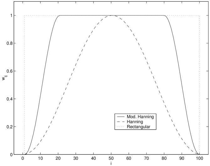
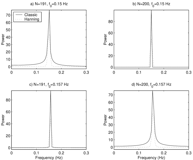
where: $\{\sigma_{i}\}$ and $\{\delta_{i}\}$ are the eigenvalues of $\boldsymbol{H}$ and $\boldsymbol{L}$, respectively, $\boldsymbol{\widehat{g}}=\boldsymbol{{\cal F}}\boldsymbol{g}$, with $\boldsymbol{{\cal F}}$ the bidimensional Fourier matrix, and $n$ is the number of pixels in the image. To reduce edge effects on $\boldsymbol{\widehat{g}}$ we use an estimate of $\|\,\boldsymbol{\widehat{g}}\,\|^{2}$ (the spectrum) based on bidimensional windowing of the Fourier transform: $\boldsymbol{\widehat{g}}$ is estimated via $\boldsymbol{\tilde{g}}_{1}=\boldsymbol{{\cal F}}(\boldsymbol{w}_{1}\odot\boldsymbol{g})$, where “ $\odot$ ” denotes element-wise matrix multiplication and $\boldsymbol{w}_{1}$ is a bidimensional function (window) tapered smoothly to zero at the image edges. A typical choice for $\boldsymbol{w}_{1}$ is the Hanning window (see Fig. 1), but many other alternatives are available. The need for windowing is evident in Fig. 2, which shows a simple example based on the realization of a pure sinusoidal process. It is clear that without windowing the (classic) estimated power-spectrum of the signal strongly depends on the the specific sampling pattern. Note the spread of power at all the frequencies, visible in panels ${\rm(a)}$ and ${\rm(d)}$, which has deleterious effects in regularization parameter estimates. Windowing stabilizes the power-spectrum estimates.

Once the parameter $\lambda$ is estimated, a second windowing is necessary to also reduce edge effects in the deblurring stage, i.e., the deblurring operation has to be carried out on a windowed map $\boldsymbol{\tilde{g}}_{2}=\boldsymbol{{\cal F}}(\boldsymbol{w}_{2}\odot\boldsymbol{g})$. In this step, however, $\boldsymbol{w}_{2}$ should distort the map as little as possible. A possible solution is a window that does not alter the image within a central subimage. We use the following modification of the classic Hanning window

$$(w_{2})_{ij}=\left\{\begin{array}[]{ll}0.25\times\alpha\times\beta&1\leq i,j\leq N_{w};\\ w_{(N-i+1)(N-j+1)}&N-N_{w}<i,j\leq N;\\ 1&{\rm otherwise};\end{array}\right.$$ (15)

where $\alpha=[1-\cos(\pi\leavevmode\nobreak\ (i-1)/N_{w})]$, and $\beta=[1-\cos(\pi\leavevmode\nobreak\ (j-1)/N_{w})]$ so that the pixels in the central subimage are not modified and the image has continuous first derivatives at the edges (see Fig. 1). This window approaches the classic two-dimensional Hanning window as $N_{w}\rightarrow N/2$ and tends to the rectangular windows as $N_{w}\rightarrow 0$. The parameter $N_{w}$ thus determines the filtering characteristics, in particular the frequency pass-band, of the window. Its “optimal” value depends on many factors such as the noise level, the form of the PSF and the specific realization of the process.

5 Reflexive image extension

Another method that allows, at least in principle, the use of reflexive BC with asymmetric PSFs and which does not require discarding any data, consists of extending the original image $X$ according to the scheme

$$\begin{array}[]{ccc}X_{rc}&X_{r}&X_{rc}\\ X_{c}&X&X_{c}\\ X_{rc}&X_{r}&X_{rc}\end{array}$$

where $X_{c}$ is obtained by “flipping” the columns of $X$, $X_{r}$ is obtained by “flipping” the rows of $X$, and $X_{rc}$ is obtained by “flipping” the rows and columns of $X$. Since the resulting image is periodic, periodic BC can be used without introducing discontinuities. However the computational cost is higher as the new image is nine times larger. A more feasible approach is to make $X_{rc}$, $X_{c}$, and $X_{r}$ only part of the image, say bands of thickness $N_{{\rm ext}}$ of the same order as the width of the PSF. Since the discontinuities introduced by the BC are expected mainly at the edges, this image extension keeps edge effects on a part of the image that is later discarded. This method, however, has the disadvantage of not providing full reflexive BC and thus it has to be implemented using a windowing operation similar to that presented in Sect.4 with $N_{w}=N_{{\rm ext}}$.

Figure 1: Slice comparison of the two-dimensional classical Hanning and rectangular windows with the modified Hanning window ($N_{w}=20$).

Figure 2: Power-Spectra of four different realizations of the process $x[t]=\sin(2\pi f_{0}t)$, $t=0,1,\ldots,N$ for $f_{0}=0.150$ and $0.157\leavevmode\nobreak\ {\rm Hz}$, $N=191$ and $200$. The true power-spectrum (not shown) is a $\delta$-function centered at $f_{0}$.

	Wiener		Ref. Ext.		Tikhonov		Wind. Ref. Ext.		Wind. Tikh.		Kron. Approx.
${\rm S/N}$	${\rm rrms\,(\%)}$		${\rm rrms\,(\%)}^{\mathrm{a}}$		${\rm rrms\,(\%)}$		${\rm rrms\,(\%)}^{\mathrm{a}}$		${\rm rrms\,(\%)}$		${\rm rrms\,(\%)}^{\mathrm{a}}$
2	$50.71\pm 0.12$		$51.09\pm 0.20$		$50.18\pm 0.21$		$50.99\pm 0.18$		$49.99\pm 0.20$		$52.37\pm 0.37$
10	$45.64\pm 0.07$		$52.01\pm 0.39$		$47.08\pm 0.28$		$50.90\pm 0.37$		$45.50\pm 0.13$		$*$
100	$41.29\pm 0.04$		$*$		$*$		$*$		$42.83\pm 0.19$		$*$

Table 1: Summary of the results obtained for a simulated sky map contaminated with $100$ different realization of a white noise process at the PLANK-LFI frequencies and axial ratio of the elliptical PSF equal to $1:1.3$ (see text). The central $300\times 300$ pixels of the images are considered. The original maps consisted of $364\times 364$ pixels, i.e., a border of $32$ pixels has been removed from each side of the images, corresponding to about four times the dispersion of the PSF along the major axis. $N_{w}=32$ for the modified Hanning window used for the windowed reflexive expansion and the windowed Tikhonov methods and for the calculation of the regularization parameter in the reflexive expansion and Tikhonov methods (see text). All of the methods have adopted a discrete Laplacian for $\boldsymbol{L}$ and ( except for the Kronecker approximation) periodic BCs. The Kronecker approximation uses reflexive BCs. The relative root mean square (rrms) is defined as the ratio of the residual root mean square (rms) to the rms of the true signal. The asterisk means unstable results.

• Calculated on full $364\times 364$ pixel images.

	Wiener		Ref. Ext.		Tikhonov		Wind. Ref. Ext.		Wind. Tikh.		Kron. Approx.
${\rm S/N}$	${\rm rrms\,(\%)}$		${\rm rrms\,(\%)}^{\mathrm{a}}$		${\rm rrms\,(\%)}$		${\rm rrms\,(\%)}^{\mathrm{a}}$		${\rm rrms\,(\%)}$		${\rm rrms\,(\%)}^{\mathrm{a}}$
2	$48.42\pm 0.12$		$49.21\pm 0.18$		$47.98\pm 0.17$		$48.97\pm 0.16$		$47.91\pm 0.17$		$56.82\pm 0.72$
10	$43.35\pm 0.07$		$52.50\pm 0.50$		$44.56\pm 0.22$		$50.86\pm 0.45$		$43.19\pm 0.13$		$*$
100	$38.90\pm 0.04$		$*$		$*$		$*$		$39.67\pm 0.14$		$*$

Table 2: As in Table 1 with the axial ratio of the elliptical PSF equal to to $1:2$

	Wiener		Ref. Ext.		Tikhonov		Wind. Ref. Ext.		Wind. Tikh.		Kron. Approx.
${\rm S/N}$	${\rm rrms\,(\%)}$		${\rm rrms\,(\%)}^{\mathrm{a}}$		${\rm rrms\,(\%)}$		${\rm rrms\,(\%)}^{\mathrm{a}}$		${\rm rrms\,(\%)}$		${\rm rrms\,(\%)}^{\mathrm{a}}$
2	$51.04\pm 0.55$		$51.91\pm 0.56$		$50.64\pm 0.62$		$51.85\pm 0.55$		$50.60\pm 0.63$		$51.17\pm 0.65$
10	$45.73\pm 0.38$		$52.81\pm 1.15$		$47.11\pm 0.74$		$51.91\pm 1.07$		$45.56\pm 0.41$		$*$
100	$41.12\pm 0.26$		$*$		$*$		$*$		$42.65\pm 0.38$		$*$

Table 3: As in Table 1 with the only difference that a new Gaussian random field is generated for each simulation.

	Wiener		Ref. Ext.		Tikhonov		Wind. Ref. Ext.		Wind. Tikh.		Kron. Approx.
${\rm S/N}$	${\rm rrms\,(\%)}$		${\rm rrms\,(\%)}^{\mathrm{a}}$		${\rm rrms\,(\%)}$		${\rm rrms\,(\%)}^{\mathrm{a}}$		${\rm rrms\,(\%)}$		${\rm rrms\,(\%)}^{\mathrm{a}}$
2	$48.63\pm 0.50$		$49.99\pm 0.51$		$48.32\pm 0.57$		$49.75\pm 0.50$		$48.28\pm 0.57$		$57.20\pm 1.11$
10	$43.23\pm 0.33$		$52.61\pm 1.32$		$44.12\pm 0.54$		$51.52\pm 1.13$		$43.10\pm 0.36$		$*$
100	$38.62\pm 0.22$		$*$		$*$		$*$		$39.33\pm 0.27$		$*$

Table 4: As in Table 2 with the only difference that a new Gaussian random field is generated for each simulation.

6 Numerical experiments

6.1 A preliminary experiment

Figure 3: Grayscale image of the central $290\times 290$ pixels of a simulated sky map at the PLANCK-LFI frequencies with ${\rm S/N}=2$ and axial ratio of the elliptical PSF equal to $1:1.3$ (see text). The original map was of $354\times 354$ pixels, i.e., a border of $32$ pixels has been removed from each side of the image, corresponding to about four times the dispersion of the PSF along the major axis. $N_{w}=32$ has been used for the dewindowed modified Hanning methods as well as Periodic BC and discrete Laplacian for $\boldsymbol{L}$. For the approximated Kronecker method a reflexive BC has been adopted.

Figure 4: As in Fig. 3 but with ${\rm S/N}=10$ and axial ratio $=1:1.3$.

Figure 5: As in Fig. 3 but with ${\rm S/N}=2$ and axial ratio $=1:2$.

Figure 6: As in Fig. 4 but with ${\rm S/N}=10$ and axial ratio $=1:2$.

To support our arguments and study the performance of the approximations and methods described in the previous sections, we present the result of numerical simulations based on a Gaussian random process with statistical characteristics similar to those expected for the CMB emission at the frequencies typical of PLANCK-LFI (see VNT). The PSF is Gaussian with elliptical symmetry, the FWHM along the major axis is $\approx 8$ pixels (about two times the worst spatial resolution expected for PLANCK), and with axes forming an angle of $45^{\circ}$ with the edges of the map. We consider the ${\rm S/N}$ ratios $2$, $10$, $100$; and two values of the axial ratio: $1:1.3$ and $1:2$. The axial ratios and the width of the PSF used in the experiment are by far less favorable than those expected for PLANCK and represent a sort of worst possible scenario. The reason for using ${\rm S/N}$ ratios much more larger than the value expected for PLANCK ($\approx 2$) is that some characteristics of the method are hidden by high noise contamination. Six deblurring methods are tested: classic Wiener, Tikhonov (with periodic BC and discrete Laplacian for $\boldsymbol{L}$) applied both to $\boldsymbol{\widehat{g}}$ and $\boldsymbol{\tilde{g}}$ (windowed Tikhonov), reflexive extension method (with periodic BC and discrete Laplacian for $\boldsymbol{L}$) applied both to a windowed and to an unwindowed extended image, and the Kronecker approximation with reflexive BC. Since the random field is Gaussian and stationary and the noise is assumed white, classical Wiener filtering is expected to provide the smallest mean square error among linear filters. However, this filter requires knowledge of the spectrum of the unknown signal which is not available in practice. We use Wiener deblurring, based on the real spectrum of the signal, as a sort of benchmark to assess the performance of Tikhonov methods. For this reason, it has also been implemented in a way that avoids edge effects.

The simulations have been conducted under two different scenarios. We first fix the sky and generate different realizations of the noise process. Then, to account for the variability of the random field, we simulate different realizations of the random field and the noise process.

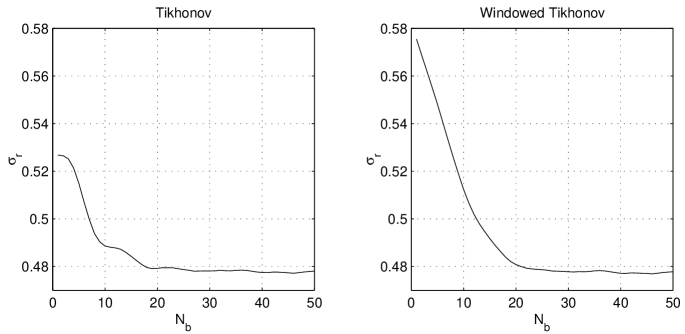
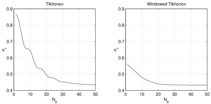
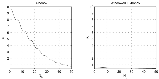
Tabs.1-4 and Figs.3-6 confirm that the Kronecker approximation method does not perform well with a very asymmetric PSF. Furthermore, it is evident that the windowed Tikhonov method performs the best, close to the Wiener filter, even in the case of very high ${\rm S/N}$ that is troublesome for the other methods. Figs. 7-9 show the typical behavior of the standard deviation of the residuals of the deblurred and the true maps as larger borders are removed from the frames. The effect of the Gibbs phenomenon is evident in the figures, especially those obtained by directly deblurring the unwindowed $\boldsymbol{\widehat{g}}$ and for high values of ${\rm S/N}$. These figures indicate that for moderate ${\rm S/N}$ ratios a border of thickness $3$-$4$ times the dispersion of the PSF has to be removed after the deblurring to reduce edge effects. By increasing $N_{w}$, this method still performs better even for very high ${\rm S/N}$ ratios. In typical CMB applications the ${\rm S/N}$ is low, thus here we do not consider the question of finding an “optimal” value of $N_{w}$. In fact, our simulations indicate that a value of $N_{w}$ equal to $3$-$4$ times the dispersion of the PSF along the major axis is a reasonable choice. This value corresponds approximately to the thickness of the border in which the blurred image is influenced by data outside of the field of view.

Finally, as shown in Tables 1-4, the methods provide similar results for low ${\rm S/N}$ ratios, especially when a sufficiently large number of edge pixels is removed from the image. This is not surprising as edge effects remain close to the edges and high noise levels hide the effects of the smallest eigenvalues of $\boldsymbol{H}$ that cause the ill-posedness of the deblurring operation.

Figure 7: Standard deviation $\sigma_{r}$ of the residual between the deblurred and the true maps vs. the width $N_{b}$ of the removed border for the map in Fig. 5

.

Figure 8: Standard deviation $\sigma_{r}$ of the residual between the deblurred and the true maps vs. the width $N_{b}$ of the removed border for the map in Fig. 6

.

Figure 9: As in Figs. 7 and 8 but with ${\rm S/N}=100$

.

Tables 5 and 6 show the results of $100$ simulations similar to those presented previously but under the conditions expected for PLANCK-LFI. As expected, given the low ${\rm S/N}$ ratio, the performance of the various methods is similar.

	Wiener			Windowed Tikhonov				Kronecker Approx.
${\rm FWHM\,(arc.min.)}$		${\rm rrms\,(\%)}$		${\rm rrms\,(\%)}$		$\lambda$		${\rm rrms\,(\%)}^{\mathrm{a}}$		$\lambda$
$10$		$30.36\pm 0.06$		$30.35\pm 0.06$		$0.69\pm 0.02$		$30.45\pm 0.05$		$0.69\pm 0.01$
$14$		$32.64\pm 0.07$		$36.68\pm 0.09$		$0.79\pm 0.04$		$37.96\pm 0.08$		$0.79\pm 0.04$
$23$		$36.74\pm 0.08$		$36.68\pm 0.09$		$0.79\pm 0.04$		$36.96\pm 0.08$		$0.79\pm 0.02$
$33$		$40.54\pm 0.10$		$40.47\pm 0.11$		$0.77\pm 0.04$		$40.70\pm 0.11$		$0.79\pm 0.02$

Table 5: Summary of the results concerning the deblurring of a sky map contaminated with $100$ realizations of a Gaussian random process whose statistical properties are similar to those expected of the CMB sky observed with four channels of PLANCK-LFI for beams with elliptical symmetry. The central $320\times 320$ pixels of the images are considered. The original maps consisted of $350\times 350$ pixels (corresponding to a sky area of about $20^{\circ}\times 20^{\circ}$), i.e., a border of $15$ pixels has been removed from each side of the images. The techniques used are Wiener filtering, windowed Tikhonov (with periodic boundary conditions and discrete Laplacian for $\boldsymbol{L}$) and the Kronecker approximation (with reflexive boundary conditions and discrete Laplacian for $\boldsymbol{L}$). Here ${\rm S/N=2}$, ${\rm FWHM}$ is the full width at half maximum along the major axis of the PSF, the axial ratio for the PSF is $1:1.3$ and $N_{w}=15$. The relative root mean square (rrms) is defined as the ratio of the residual root mean square (rms) to the rms of the true signal. When applicable, the mean values and dispersions of the GCV estimates of $\lambda$ are also shown.

• Calculated on the entire images of $350\times 350$ pixels.

	Wiener			Windowed Tikhonov				Kronecker Approx.
${\rm FWHM\,(arc.min.)}$		${\rm rrms\,(\%)}$		${\rm rrms\,(\%)}$		$\lambda$		${\rm rrms\,(\%)}^{\mathrm{a}}$		$\lambda$
$10$		$30.68\pm 0.26$		$30.71\pm 0.29$		$0.73\pm 0.03$		$30.73\pm 0.28$		$0.73\pm 0.03$
$14$		$32.68\pm 0.24$		$32.68\pm 0.28$		$0.75\pm 0.04$		$32.73\pm 0.27$		$0.76\pm 0.04$
$23$		$36.74\pm 0.24$		$36.67\pm 0.28$		$0.78\pm 0.04$		$36.78\pm 0.26$		$0.79\pm 0.04$
$33$		$40.65\pm 0.27$		$40.52\pm 0.30$		$0.77\pm 0.05$		$40.73\pm 0.29$		$0.81\pm 0.05$

Table 6: As in Table 5 with the only difference that a new Gaussian random field is generated for each simulation.

6.2 Numerical simulations with realistic CMB maps

The next step is to test the performance of the deblurring procedure with realistic CMB maps from the point of view of the angular power spectrum. As usual, it is defined as the set of coefficients $C_{\ell}$ of the two-point correlation function expanded in Legendre polynomials; $\ell$ marks the power at the angular scale given approximately by $\theta\simeq 180/\ell$. We compare the quality of the reconstruction with the corresponding one in VNT, which assumed a circular Gaussian beam.

We consider the same templates as in VNT: the region is a squared patch ($350\times 350$ pixels) with side of about $20^{\circ}$, centered at $l=90^{\circ}$, $b=45^{\circ}$ (Galactic coordinates). The latitude is high enough that CMB emission dominates over foregrounds, assumed to be represented by synchrotron (Haslam et al. 1982) and dust (Schlegel et al. 1998) emission. We neglect contributions of point sources. The CMB model, in agreement with current experimental results (de Bernardis et al. 2002; Halverson et al. 2002; Lee et al. 2001), corresponds to a flat Friedmann-Robertson-Walker (FRW) metric with a cosmological constant ($70\%$ of the critical density), Hubble parameter today $H_{0}=100h$ km/sec/Mpc with $h=0.7$ baryons at $5\%$ and Cold Dark Matter (25% CDM), with a scale-invariant Gaussian initial spectrum of adiabatic density perturbations.

The PLANCK-LFI instrument works at frequencies $30$, $44$, $70$, and $100\leavevmode\nobreak\ {\rm GHz}$. We assume nominal noise and angular resolution corresponding to the four frequencies $30$, $44$, $70$, and $100\leavevmode\nobreak\ {\rm GHz}$ at which the PLANCK-LFI instrument works. The simulated maps are blurred through Gaussian PSF’s with elliptical symmetry. In particular, the following FWHM’s along the major axis have been used: $\approx 33^{\prime}$ at $30\leavevmode\nobreak\ {\rm GHz}$, $\approx 23^{\prime}$ at $44\leavevmode\nobreak\ {\rm GHz}$, $\approx 14^{\prime}$ at $70\leavevmode\nobreak\ {\rm GHz}$, $\approx 10^{\prime}$ at $100\leavevmode\nobreak\ {\rm GHz}$, with axial ratio set to $1:1.3$, and axes forming an angle of $45^{\circ}$ with the edges of the map. Simulated white noise, with rms level as expected for the considered channels, has been added to the maps. Since we choose to work with a pixel size of about $3.5$ arcminutes, the noise rms are $.042$, $.049$, $.042$ and $.043$ mK in antenna temperature at $30$, $44$, $70$, $100\leavevmode\nobreak\ {\rm GHz}$, respectively.

Again, as in VNT, we can see two important characteristics of the deblurring process: first it reconstructs the correct shape and amplitude of the part of the spectrum which is mildly affected by the PSF; second, it reconstructs part of the power where the signal is degraded substantially by the PSF and noise. In fact, we see that the performance of the deblurring method is almost the same as that reported in VNT for symmetric PSF. Indeed, in the $30$, $44$, $70$ and $100\leavevmode\nobreak\ {\rm GHz}$ cases the spectrum is reconstructed up to $\ell\simeq 400$, $500$, $700$ and $800$ respectively.

We conclude that, for what concerns the power spectrum analysis, the proposed technique seems to work well also with asymmetric shapes of the instrumental beam.

Note also that for a fixed $\lambda$ the Tikhonov estimate (3) is a linear function of the data and therefore the covariance matrix of the deblurred field can be obtained by propagating the covariance matrix of the original field through the linear operators. Even if the GCV estimate of $\lambda$ makes the estimate nonlinear, for large samples the linear approximation that assumes $\lambda$ is fixed is reasonable. In any case, it is necessary to stress that the most feasible way to account for the changes in the statistics of the CMB through any estimation process (to include the effects of, for example, edge effects, possible unremoved point sources, asymmetry and/or non-stationary PSF etc.), is probably through Monte Carlo simulations where one applies the same algorithm to the data and to simulated maps to compare and fit the best cosmological model. The low computational cost of our algorithm is certainly interesting with this respect.

7 Discussion and conclusions

We have considered Tikhonov regularization for deblurring CMB maps in real space. As shown in VNT, this approach permits the development of algorithms that are more flexible and robust than those based on frequency-space methods. The methods developed in VNT, however, apply to the case of symmetric PSFs for which efficient methods can be implemented with reflexive BC. In the present paper we have considered the more general case of asymmetric PSFs.

We have presented a method based on a Kronecker separable approximation of the PSF that can be used with mildly asymmetric PSFs. For more asymmetric cases we presented a periodic BC approach that can be efficiently implemented with image windows and fast Fourier transforms. Windowing is necessary to reduce edge effect in the selection of the regularization parameter. Of course, one can easily derive a GCV function that only takes into account pixels away from the edges but the computational cost is higher.

We have applied our methodology to simulated skies at typical CMB frequencies. We considered test signals with known statistics, as well as realistic simulations of the CMB sky contaminated by noise whose rms is that expected for the low frequency instrument aboard the PLANCK satellite. This case is particularly interesting for application of a deblurring procedure, as the instrument observes the sky at 30, 44, 70 and 100 GHz with very different PSFs of resolution $33$, $22$, $14$, $10$ arcminutes. We found that the proposed methodology performs as well or better than the Wiener benchmark that relies on the true spectrum and that avoids edge effects.

Figure 10: Angular power spectrum at $30\leavevmode\nobreak\ {\rm GHz}$ in different steps of the analysis.

Figure 11: Angular power spectrum at $44\leavevmode\nobreak\ {\rm GHz}$ in different steps of the analysis.

Figure 12: Angular power spectrum at $70\leavevmode\nobreak\ {\rm GHz}$ in different steps of the analysis.

Figure 13: Angular power spectrum at $100\leavevmode\nobreak\ {\rm GHz}$ in different steps of the analysis.

References

- Baccigalupi et al. (2000) Baccigalupi, C., Bedini, L., Burigana, C. et al. 2000, MNRAS, 318, 769
- de Bernardis et al. (2002) de Bernardis, P., Ape, P.A.R., & Bock, J.J. 2002, ApJ, 564, 559
- Golub & Van Loan (1996) Golub, G.H., & Van Loan, C.F. 1996, Matrix Computations, 3rd ed. (Johns Hopkins, Baltimore)
- Halverson et al. (2002) Halverson, N.W., Leitch, E.M, & Pryke, C. 2002, ApJ, 568, 38
- Haslam et al. (1982) Haslam, C.G.T., Stoffel, H., Salter, C.J., & Wilson, W.E. 1982, A&AS, 47, 1
- Kamm & Nagy (2000) Kamm, J., & Nagy, J.G. 2000, SIAM J. Matrix Anal. and Appl., 22, 155
- Lee et al. (2001) Lee, B.C., Tucker, D.L. et al. 2001, ApJL, 561, 183
- Maino et al. (2002) Maino, D., Farusi, A., Baccigalupi, C. et al. 2002, MNRAS, 334, 53
- Nagy et al. (2002) Nagy, J.G., Ng, M.K., & Perrone, L. 2002, SIAM J. Matrix Anal. and Appl., submitted
- Schlegel et al. (1998) Schlegel, D.J., Finkbeiner, D.P., & Davies, M. 1998, ApJ, 500, 525
- Van Loan & Pitsianis (1993) Van Loan, C.F. & Pitsianis, N.P. 1993 in Moonen, M.S. & Golub, G.H. ed., Linear Algebra for Large Scale and Real Time Applications, Kluwer Publications, 293
- Tegmark (1999) Tegmark, M. 1999, ApJ, 519, 513
- Vio et al. (2003) Vio, R., Nagy, J.G., Tenorio, L. et al. 2003, A&A, 389, 404 (VNT)