Stellar population synthesis at the resolution of 2003

Abstract

We present a new model for computing the spectral evolution of stellar populations at ages between $1\times 10^{5}\,$yr and $2\times 10^{10}\,$yr at a resolution of 3 Å across the whole wavelength range from 3200 Å to 9500 Å for a wide range of metallicities. These predictions are based on a newly available library of observed stellar spectra. We also compute the spectral evolution across a larger wavelength range, from 91 Å to 160 $\mu$m, at lower resolution. The model incorporates recent progress in stellar evolution theory and an observationally motivated prescription for thermally-pulsing stars on the asymptotic giant branch. The latter is supported by observations of surface brightness fluctuations in nearby stellar populations. We show that this model reproduces well the observed optical and near-infrared colour-magnitude diagrams of Galactic star clusters of various ages and metallicities. Stochastic fluctuations in the numbers of stars in different evolutionary phases can account for the full range of observed integrated colours of star clusters in the Magellanic Clouds. The model reproduces in detail typical galaxy spectra from the Early Data Release (EDR) of the Sloan Digital Sky Survey (SDSS). We exemplify how this type of spectral fit can constrain physical parameters such as the star formation history, metallicity and dust content of galaxies. Our model is the first to enable accurate studies of absorption-line strengths in galaxies containing stars over the full range of ages. Using the highest-quality spectra of the SDSS EDR, we show that this model can reproduce simultaneously the observed strengths of those Lick indices that do not depend strongly on element abundance ratios. The interpretation of such indices with our model should be particularly useful for constraining the star formation histories and metallicities of galaxies.

1 Introduction

The star formation history of galaxies is imprinted in their integrated light. The first attempts to interpret the light emitted from galaxies in terms of their stellar content relied on trial and error analyses (e.g., Spinrad & Taylor 1971; Faber 1972; O’Connell 1976; Turnrose 1976; Pritchet 1977; Pickles 1985). In this technique, one reproduces the integrated spectrum of a galaxy with a linear combination of individual stellar spectra of various types taken from a comprehensive library. The technique was abandoned in the early 1980’s because the number of free parameters was too large to be constrained by typical galaxy spectra. More recent models are based on the evolutionary population synthesis technique (Tinsley 1978; Bruzual 1983; Arimoto & Yoshii 1987; Guiderdoni & Rocca-Volmerange 1987; Buzzoni 1989; Bruzual & Charlot 1993; Bressan, Chiosi & Fagotto 1994; Fritze-v. Alvensleben & Gerhard 1994; Worthey 1994; Leitherer & Heckman 1995; Fioc & Rocca-Volmerange 1997; Maraston 1998; Vazdekis 1999; Schulz et al. 2002). In this approach, the main adjustable parameters are the stellar initial mass function (IMF), the star formation rate (SFR) and, in some cases, the rate of chemical enrichment. Assumptions about the time evolution of these parameters allow one to compute the age-dependent distribution of stars in the Hertzsprung-Russell (HR) diagram, from which the integrated spectral evolution of the stellar population can be obtained. These models have become standard tools in the interpretation of galaxy colours and spectra.

Despite important progress over the last decade, modern population synthesis models still suffer from serious limitations. The largest intrinsic uncertainties of the models arise from the poor understanding of some advanced phases of stellar evolution, such as the supergiant phase and the asymptotic-giant-branch (AGB) phase (see Charlot 1996; Charlot, Worthey & Bressan 1996; Yi 2003). Stars in these phases are very bright and have a strong influence on integrated-light properties. The limitations arising from these uncertainties in the interpretation of galaxy spectra are further amplified by the fact that age, metallicity and dust all tend to affect spectra in similar ways. This is especially true at the low resolving power of most current population synthesis models, i.e., typically $\sim 250$ at optical wavelengths (see however Vazdekis 1999; Schiavon et al. 2002). As a result, light-weighted ages and metallicities derived from integrated galaxy spectra tend to be strongly degenerate (e.g., Worthey 1994). For old stellar populations, this degeneracy may be broken by studying surface brightness fluctuations, that are more sensitive to the details of the stellar luminosity function than ordinary integrated light (Liu et al. 2000; Blakeslee et al. 2001). This method, however, is mostly applicable to studies of nearby ellipticals and spiral bulges.

The general contention is that the age-metallicity degeneracy can be broken by appealing to refined spectral diagnostics involving individual stellar absorption-line features (e.g., Rose 1985; Jones & Worthey 1995; Vazdekis & Arimoto 1999). Several spectral indices of this kind have been defined at optical and near-infrared wavelengths (e.g., Faber 1973; Rose 1984; Díaz, Terlevich & Terlevich 1989; Worthey et al. 1994). In the widely used ‘Lick system’, the strengths of 25 spectral indices were parametrized as functions of stellar effective temperature, gravity and metallicity using a sample of 460 Galactic stars (Burstein et al. 1984; Gorgas et al. 1993; Worthey et al. 1994; Worthey & Ottaviani 1997; Trager et al. 1998). This convenient parametrization allows one to compute integrated index strengths of model galaxies with any stellar population synthesis code. In practice, however, the applications are limited to studies of old stellar populations because of the lack of hot stars in the Lick stellar library. Also, the Lick indices were defined in spectra which were not flux-calibrated and whose resolution ($\sim 9$ Å FWHM) is three times lower than achieved in modern spectroscopic galaxy surveys, such as the Sloan Digital Sky Survey (SDSS; York et al. 2000). Thus high-quality galaxy spectra must first be degraded to the specific calibration and wavelength-dependent resolution of the Lick system for Lick index-strength analyses to be performed (Section 4.4). Ideally, one requires a population synthesis model that can predict actual spectra of galaxies at the resolution of modern surveys. The model of Vazdekis (1999) fulfills this requirement. However, it is limited to two narrow wavelength regions, 3820–4500 Å and 4780–5460 Å.

In this paper, we present a new model for computing the spectral evolution of stellar populations of different metallicities at ages between $1\times 10^{5}\,$yr and $2\times 10^{10}\,$yr at a resolution of 3 Å FWHM across the whole wavelength range from 3200 Å to 9500 Å (corresponding to a median resolving power $\lambda/\Delta\lambda\approx 2000$). These predictions are based on a new library of observed stellar spectra recently assembled by Le Borgne et al. (2003). We also compute the spectral evolution across a larger wavelength range, from 91 Å to 160 $\mu$m, at lower spectral resolution. This model should be particularly useful for interpreting the spectra gathered by modern spectroscopic surveys in terms of constraints on the star formation histories and metallicities of galaxies.

The paper is organized as follows. In Section 2 below, we present the stellar evolution prescription and the stellar spectral library on which our model relies. We consider several alternatives for these ingredients. We adopt an observationally motivated prescription for thermally-pulsing AGB stars, which is supported by observations of surface brightness fluctuations in nearby stellar populations (Liu et al. 2000; Liu, Graham & Charlot 2002). We also briefly recall the principle of the isochrone synthesis technique for computing the spectral evolution of stellar populations (Charlot & Bruzual, 1991). In Section 3, we investigate the influence of the main adjustable parameters of the model on photometric predictions and compare our results with previous work. Comparisons with observed colour-magnitude diagrams and integrated colours of star clusters of various ages and metallicities are also presented in this section. In Section 4, we compute the spectral evolution of stellar populations and compare our model with observed galaxy spectra from the SDSS EDR (Stoughton et al., 2002). We compare in detail the predicted and observed strengths of several absorption-line indices and identify those indices that appear to be most promising for constraining the stellar content of galaxies. We summarize our conclusions in Section 5, where we also suggest ways of including the effects of gas and dust in the interstellar medium on the stellar radiation computed with our model. Readers interested mainly in the photometric predictions of the model may skip directly to Section 3, while those interested mainly in applications of the model to interpret galaxy spectra may skip directly to Section 4.

2 The Model

In this section, we present the main two ingredients of our population synthesis model: the stellar evolution prescription and the stellar spectral library. We consider several alternatives for each of these. We also briefly review the principle of the isochrone synthesis technique for computing the spectral evolution of stellar populations.

2.1 Stellar evolution prescription

To account for current uncertainties in the stellar evolution theory, we consider three possible stellar evolution prescriptions in our model (Table 1). We first consider the library of stellar evolutionary tracks computed by Alongi et al. (1993), Bressan et al. (1993), Fagotto et al. (1994a), Fagotto et al. (1994b), and Girardi et al. (1996). This library encompasses a wide range of initial chemical compositions, $Z=0.0001$, 0.0004, 0.004, 0.008, 0.02, 0.05, and 0.1 with $Y=2.5Z+0.23$ ($Z_{\odot}=0.02$ and $Y_{\odot}=0.28$) assumed. The range of initial masses is $0.6\leq m\leq 120\,M_{\sun}$ for all metallicities, except for $Z=0.0001$ ($0.6\leq m\leq 100\,M_{\sun}$) and $Z=0.1$ ($0.6\leq m\leq 9\,M_{\sun}$). The tracks were computed using the radiative opacities of Iglesias, Rogers & Wilson (1992) and include all phases of stellar evolution from the zero-age main sequence to the beginning of the thermally pulsing regime of the asymptotic giant branch (TP-AGB; for low- and intermediate-mass stars) and core-carbon ignition (for massive stars). For solar composition, the models are normalized to the temperature, luminosity, and radius of the Sun at an age of 4.6 Gyr. The tracks include mild overshooting in the convective cores of stars more massive than $1.5\,M_{\odot}$, as suggested by observations of Galactic star clusters (Bressan et al. 1993; Meynet, Mermilliod & Maeder 1993; Demarque, Sarajedini & Guo 1994). For stars with masses between 1.0 and 1.5$\,M_{\odot}$, core overshooting is included with a reduced efficiency. Overshooting is also included in the convective envelopes of low- and intermediate-mass stars, as suggested by observations of the red giant branch and horizontal branch of star clusters in the Galactic halo and the Large Magellanic Cloud (hereafter LMC; Alongi et al. 1991). We refer to this set of tracks as the ‘Padova 1994 library’.

Table 1: Different stellar evolution prescriptions.

Name	Metallicity range	Source
Padova 1994	0.0001–0.10	Alongi et al. (1993)
		Bressan et al. (1993)
		Fagotto et al. (1994a)
		Fagotto et al. (1994b)
		Girardi et al. (1996)
Padova 2000	0.0004–0.03	Girardi et al. (2000)a
Geneva	0.02	Schaller et al. (1992)
		Charbonnel et al. (1996)
		Charbonnel et al. (1999)

${}^{a}\,$Girardi et al. (2000) computed tracks only for low- and intermediate-mass stars. In the Padova 2000 library, these calculations are supplemented with high-mass tracks from the Padova 1994 library, as suggested by Girardi et al. (2002).

Recently, Girardi et al. (2000) produced a new version of this library, in which the main novelties are a revised equation of state (Mihalas et al., 1990) and new low-temperature opacities (Alexander & Ferguson, 1994). The revised library includes stars with masses down to $m=0.15\,M_{\odot}$, but it does not contain stars more massive than $7\,M_{\odot}$ (the new equation of state affects mainly the evolution of stars less massive than $0.6\,M_{\odot}$). The chemical abundances also differ slightly from those adopted in the 1994 release, $Z=0.0004$, 0.004, 0.008, 0.019, and 0.03, with $Y=2.25Z+0.23$ ($Z_{\odot}=0.019$ and $Y_{\odot}=0.273$) assumed. Following the arguments of Girardi et al. (2002), we combine the new library of low- and intermediate-mass tracks with high-mass tracks from the older Padova 1994 library to build an updated library encompassing a complete range of initial stellar masses. This can be achieved at all but the highest metallicity ($Z=0.03$), for which there is no counterpart in the Padova 1994 library ($Z=0.02$ and 0.05 available only). We refer to this set of tracks as the ‘Padova 2000 library’.

The third stellar evolution prescription we consider, for the case of solar metallicity only, is the comprehensive library of tracks computed by Schaller et al. (1992, for $m\geq 2\,M_{\odot}$), Charbonnel et al. (1996, for $0.8\leq m<2\,M_{\sun}$) and Charbonnel et al. (1999, for $0.6\leq m<0.8\,M_{\sun}$). The abundances are $X=0.68$, $Y=0.30$, and $Z=0.02$, and the opacities are from Rogers & Iglesias (1992, for $m\geq 2\,M_{\odot}$) and Iglesias & Rogers (1993, for $0.8\leq m/M_{\odot}<2$). The tracks include all phases of stellar evolution from the zero-age main sequence to the beginning of the TP-AGB or core-carbon ignition, depending on the initial mass. The models are normalized to the luminosity, temperature, and radius of the Sun at an age of 4.6 Gyr. Mild overshooting is included in the convective cores of stars more massive than $1.5\,M_{\odot}$. Differences with the solar-metallicity calculations of Bressan et al. (1993) in the Padova 1994 library include: the absence of overshooting in the convective cores of stars with masses between 1.0 and 1.5$\,M_{\odot}$ and in the convective envelopes of low- and intermediate-mass stars; the higher helium fraction; the inclusion of mass loss along the red giant branch; the treatment of convection during core-helium burning; and the internal mixing and mass loss of massive stars. The signatures of these differences in the stellar evolutionary tracks have been investigated by Charlot et al. (1996). We refer to this alternative set of tracks for solar metallicity as the ‘Geneva library’.

We supplement the Padova and Geneva tracks of low- and intermediate-mass stars beyond the early-AGB with TP-AGB and post-AGB evolutionary tracks. The TP-AGB phase is one of the most difficult evolutionary phases to model because of the combined effects of thermal pulses (i.e., helium shell flashes), changes in surface abundance caused by heavy element dredge-up (e.g., carbon) and important mass loss terminated by a superwind and the ejection of the stellar envelope (see the reviews by Habing 1995 and Habing 1996). This phase must be included in population synthesis models because the stochastic presence of a few TP-AGB stars has a strong influence on the integrated colours of star clusters (e.g., Frogel, Mould & Blanco 1990; Santos & Frogel 1997; see also Section 3.3.2 below). We appeal to recent models of TP-AGB stars which have been calibrated using observations of stars in the Galaxy, the LMC and the Small Magellanic Cloud (SMC). In particular, we adopt the effective temperatures, bolometric luminosities and lifetimes of TP-AGB stars from the multi-metallicity models of Vassiliadis & Wood (1993). These models, which include predictions for both the optically-visible and the superwind phases, predict maximum TP-AGB luminosities in good agreement with those observed in Magellanic Cloud clusters. The models are for the metallicities $Z=0.001$, 0.004, 0.008, and 0.016, which do not encompass all the metallicities in the Padova track library. For simplicity, we adopt the $Z=0.001$ prescription of Vassiliadis & Wood (1993) at all metallicities $Z\leq 0.0004$ and their $Z=0.016$ prescription at all metallicities $Z\geq 0.02$.

Carbon dredge-up during TP-AGB evolution can lead to the transition from an oxygen-rich (M-type) to a carbon-rich (C-type) star (e.g., Iben & Renzini 1983). Since C-type stars are much redder than M-type stars and can dominate the integrated light of some star clusters, it is important to include them in the models. The minimum initial mass limit for a carbon star to form increases with metallicity. This is supported observationally by the decrease in the ratio of C to M stars from the SMC, to the LMC, to the Galactic bulge (Blanco, Blanco & McCarthy, 1978). While the formation of carbon stars is relatively well understood, no simple prescription is available to date that would allow us to describe accurately the transition from M to C stars over a wide range of initial masses and metallicities. Groenewegen & de Jong (1993) and Groenewegen, van den Hoek & de Jong (1995) have computed models of TP-AGB stars, which reproduce the ratios of C to M stars observed in the LMC and the Galaxy. We use these models to define the transition from an M-type star to a C-type star in the TP-AGB evolutionary tracks of Vassiliadis & Wood (1993). We require that, for a given initial main-sequence mass, the relative durations of the two phases be the same as those in the models of Groenewegen & de Jong (1993) and Groenewegen et al. (1995). Since these models do not extend to sub-Magellanic ($Z\la 0.004$) nor super-solar ($Z>0.02$) metallicities, we apply fixed relative durations of the M-type and C-type phases in the Padova tracks for more extreme metallicities. As shown by Liu et al. (2000), this simple but observationally motivated prescription for TP-AGB stars provides good agreement with the observed optical and near-infrared surface brightness fluctuations of (metal-poor) Galactic globular clusters and (more metal-rich) nearby elliptical galaxies.

For the post-AGB evolution, we adopt the evolutionary tracks of Vassiliadis & Wood (1994), whose calculations cover the range of metallicities $0.001\leq Z\leq 0.016$. We use the Weidemann (1987) relationship to compute the core mass of a star after ejection of the planetary nebula (PN) at the tip of the AGB from its initial mass on the main sequence (see Weidemann 1990 for a review; and Magris & Bruzual 1993). To each low- and intermediate-mass star in the Padova and Geneva libraries, we then assign the post-AGB evolution computed by Vassiliadis & Wood (1994) corresponding to the closest core mass and metallicity. These authors did not consider the evolution of stars with core masses less than $0.569\,M_{\odot}$, corresponding to a main sequence progenitor mass less than about $1.1\,M_{\odot}$. For lower-mass stars, we adopt the $0.546\,M_{\odot}$ post-AGB evolutionary track computed for the metallicity $Z=0.021$ by Schönberner (1983), with an extension by Köster & Schönberner (1986). Since we will consider stellar population ages of up to 20 Gyr, and the post-AGB calculations do not generally extend to this limit, we further supplement the tracks using white dwarf cooling models by Winget et al. (1987) at luminosities $L\la 0.1L_{\odot}$. Following the suggestion by Winget et al., we adopt their ‘pure carbon’ models for masses in the range $0.4\leq m\leq 1.0\,M_{\sun}$, in which the cooling times differ by only 15 per cent from those in models including lighter elements. The prescription is thus naturally independent of the metallicity of the progenitor star. Specifically, we interpolate cooling ages for white dwarfs as a function of luminosity at the masses corresponding to the Vassiliadis & Wood (1994) and Schönberner (1983) tracks. Since Winget et al. (1987) do not tabulate the temperatures nor the radii of their model white dwarfs, we assign effective temperatures as a function of luminosity using the slope of the white dwarf cooling sequence defined by the calculations of Schönberner (1983), i.e., $\Delta\log T_{\rm eff}\approx 0.23\Delta\log L$.

The resulting tracks in the Padova and Geneva libraries cover all phases of evolution from zero-age main sequence to remnant stage for all stars more massive than $0.6\,M_{\odot}$ ($0.15\,M_{\odot}$ for the Padova 2000 library). Since the main-sequence lifetime of a $0.6\,M_{\odot}$ star is nearly 80 Gyr, we supplement these libraries with multi-metallicity models of unevolving main-sequence stars in the mass range $0.09\leq m<0.6\,M_{\sun}$ (Baraffe et al., 1998). These models provide smooth extensions of the Padova and Geneva calculations into the lower main sequence. For the purpose of isochrone synthesis, all tracks must be resampled to a system of evolutionary phases of equivalent physical significance (Charlot & Bruzual, 1991). We define 311 such phases for low- and intermediate-mass stars and 260 for massive stars.

2.2 Stellar spectral library and spectral calibration

The second main ingredient of population synthesis models is the library of individual stellar spectra used to describe the properties of stars at any position in the Hertzsprung-Russell diagram. We consider different alternative stellar spectral libraries and different ways to calibrate them (see Tables 2 and 3). We also refer the reader to Table 7 of Appendix A for a qualitative assessment of the spectral predictions of our model for simple stellar populations of various ages and metallicities computed using different spectral libraries.

Table 2: Different libraries of stellar spectra.

Name	Type	Wavelength	Median	Metallicity	Source
		range	resolving power	range
BaSeL	theoretical	91 Å to 160 $\mu$m	300	$10^{-5}Z_{\sun}$ to $10Z_{\sun}$	Kurucz (1995, priv. comm.)
					Bessell et al. (1989)
					Bessell et al. (1991)
					Fluks et al. (1994)
					Allard & Hauschildt (1995)
					Rauch (2002)
STELIB	observational	3200 Å to 9500 Å	2000	$-2.0<\hbox{\rm[Fe/H]}<+0.50$	Le Borgne et al. (2003)
Pickles	observational	1205 Å to 2.5 $\mu$m	500	$Z_{\sun}$	Pickles (1998)
					Fanelli et al. (1992)

2.2.1 Multi-metallicity theoretical and semi-empirical libraries at low spectral resolution

Theoretical model atmospheres computed for wide ranges of stellar effective temperatures, surface gravities and metallicities allow one to describe the spectral energy distribution of any star in the HR diagram. Lejeune, Cuisinier & Buser (1997) and Lejeune, Cuisinier & Buser (1998) have compiled a comprehensive library of model atmospheres for stars in the metallicity range $10^{-5}Z_{\odot}\la Z\la 10\,Z_{\odot}$, encompassing all metallicities in the Padova track libraries (Section 2.1). The spectra cover the wavelength range from 91 Å to 160 $\mu$m at resolving power $\lambda/\Delta\lambda\approx 200-500$. The library consists of Kurucz (1995, private communication to R. Buser) spectra for the hotter stars (O–K), Bessell et al. (1989), Bessell et al. (1991) and Fluks et al. (1994) spectra for M giants, and Allard & Hauschildt (1995) spectra for M dwarfs.

There are three versions of this library. The first version contains the model spectra as originally published by their builders, only rebinned on to homogeneous scales of fundamental parameters (effective temperature, gravity, metallicity) and wavelength. We refer to this library as the ‘BaSeL 1.0 library’. In a second version of the library, Lejeune et al. (1997) corrected the original model spectra for systematic deviations that become apparent when $UBVRIJHKL$ colour-temperature relations computed from the models are compared to empirical calibrations. These semi-empirical blanketing corrections are especially important for M-star models, for which molecular opacity data are missing. The correction functions are expected to depend on the fundamental model parameters: temperature, gravity and metallicity. However, because of the lack of calibration standards at non-solar metallicities, Lejeune et al. (1997) applied the blanketing corrections derived at solar metallicity to models of all metallicities. While uncertain, this procedure ensures that the differentiation of spectral properties with respect to metallicity is at least the same as in the original library (and hence not worsened; see Lejeune et al. 1997 for details). This constitutes the ‘BaSeL 2.2 library’. Finally, Westera (2001) and Westera et al. (2002) recently produced a new version of the library, in which they derived semi-empirical corrections for model atmospheres at non-solar metallicities using metallicity-dependent $UBVRIJHKL$ colour calibrations. This new version is also free of some discontinuities affecting the colour-temperature relations of cool stars in the BaSeL 1.0 and BaSeL 2.2 libraries, which were linked to the assembly of model atmospheres from different sources. We refer to this as the ‘BaSeL 3.1’ (WLBC99) library.

Table 3: Different spectral calibrations.

Option	Calibration	Source
BaSeL 1.0	theoreticala	Lejeune et al. (1997)
		Lejeune et al. (1998)
BaSeL 2.2	semi-empiricalb	Lejeune et al. (1997)
		Lejeune et al. (1998)
BaSeL 3.1	semi-empiricalc	Westera (2000)
		Westera et al. (2002)

${}^{a}\,$Original calibration of model atmospheres included in the BaSeL library (see Table 2).
${}^{b}\,$Empirical blanketing corrections derived at solar metallicity and applied to models of all metallicities in the BaSeL library.
${}^{c}\,$Metallicity-dependent blanketing corrections.

The BaSeL libraries encompass the range of stellar effective temperatures $2000\leq T_{\rm eff}\leq 50,000\$K. Some stars can reach temperatures outside this range during their evolution. In particular, in the stellar evolutionary tracks of Section 2.1, Wolf-Rayet stars and central stars of planetary nebulae can occasionally be hotter than 50,000 K. To describe the hot radiation from these stars, we adopt the non-LTE model atmospheres of Rauch (2002) for $Z=Z_{\odot}$ and $Z=0.10\,Z_{\odot}$ that include metal-line blanketing from all elements from H to the Fe group (we thank T. Rauch for kindly providing us with these spectra). The models cover the temperature range $50,000\leq T_{\rm eff}\leq 1,000,000\$K at wavelengths between 5 and 2000 Å at a resolution of 0.1 Å. We degrade these models to the BaSeL wavelength scale and extrapolate blackbody tails at wavelengths $\lambda>2000\,$Å. We use the resulting spectra to describe all the stars with $T_{\rm eff}\geq 50,000\$K and $Z\geq 0.10\,Z_{\odot}$ in the stellar evolutionary tracks. For completeness, we approximate the spectra of stars hotter than 50,000 K at $Z=0.0004$ and $Z=0.0001$ by pure blackbody spectra. Cool white dwarfs, when they reach temperatures cooler than 2000 K, are also represented by pure blackbody spectra, irrespective of metallicity.

The BaSeL libraries do not include spectra for carbon stars nor for stars in the superwind phase at the tip of the TP-AGB. Our prescription for these stars is common to all spectral libraries in Table 2 and is described in Section 2.2.4 below.

2.2.2 Multi-metallicity observational library at higher spectral resolution

To build models with higher spectral resolution than offered by the BaSeL libraries, one must appeal to observations of nearby stars. The difficulty in this case is to sample the HR diagram in a uniform way. Recently, Le Borgne et al. (2003) have assembled a library of observed spectra of stars in a wide range of metallicities, which they called ‘STELIB’. When building this library, Le Borgne et al. took special care in optimizing the sampling of the fundamental stellar parameters across the HR diagram for the purpose of population synthesis modelling. The library contains 249 stellar spectra covering the wavelength range from 3200 Å to 9500 Å at a resolution of 3 Å FWHM (corresponding to a median resolving power $\lambda/\Delta\lambda\approx 2000$), with a sampling interval of 1 Å and a signal-to-noise ratio of typically 50 per pixel. After correction for stellar radial velocities (Le Borgne 2003, private communication), two narrow wavelength regions (6850–6950 Å and 7550–7725 Å) had to be removed from the spectra because of contamination by telluric features. For stars cooler than 7000 K, we replaced these segments in the spectra with metallicity-dependent model atmospheres computed at 3 Å resolution using the SPECTRUM code (Gray & Corbally, 1994, we thank C. Tremonti for kindly providing us with these computations based on the most recent Kurucz model atmospheres). For hotter stars, we replaced the segments with spectra from the lower-resolution library of Pickles (see below), resampled to 1 Å/pixel. These fixes are purely of cosmetic nature, and we do not use the predictions of the population synthesis models in these two narrow wavelength regions (we do not correct the STELIB spectra for the telluric feature around 8950–9075 Å that it is weaker than the other two features and falls in a noisier region of the spectra).

Most stars in the STELIB library were selected from the catalog of Cayrel de Strobel et al. (1992), which includes [Fe/H] determinations from high-resolution spectroscopic observations of stars in open and globular clusters in the Galaxy and of supergiant stars in the Magellanic Clouds. The STELIB library contains stars with metallicities in the range $-2.0<{\rm[Fe/H]}<+0.50$, spectral types from O5 to M9 and luminosity classes from I to V. The coverage in spectral type is not uniform at all metallicities (see Appendix A): hot ($T_{\rm eff}\ga 10,000\,$K) stars are under-represented at non-solar metallicities, and the library lacks very cool ($T_{\rm eff}<3200\,$K) stars at all metallicities. These limitations are not critical. The spectra of hot stars are not expected to depend strongly on metallicity because the opacities in these stars are dominated by electron scattering. Thus, the spectra of hot stars with solar metallicity should be representative of hot stars at all but the most extreme metallicities. Also, the lack of cool M-dwarf stars has a negligible influence on model predictions, because these stars do not contribute significantly to the integrated light of stellar populations (as found when adopting representative spectra for these stars; see Appendix A). For the coolest giant stars, we adopt in any case the prescription outlined in Section 2.2.4 below.

The main interest of the STELIB library is that it enables the interpretation of integrated spectra of star clusters and galaxies taken at relatively high resolution in the wavelength range 3200–9500 Å. To allow for a consistent modelling of spectral properties outside this range, we must extend the STELIB spectra at ultraviolet and infrared wavelengths using one of the spectral libraries described above. We consider three different types of extensions, corresponding to the three colour-temperature calibrations of the BaSeL 1.0, 2.2 and 3.1 libraries (Section 2.2.1). To assign STELIB spectra to stars on the evolutionary tracks, we therefore proceed as follows (the reader is referred to Appendix A for more detail). We first distribute the stars in several metallicity bins centered on the metallicities for which tracks are available (Section 2.1). Some stars with intermediate metallicities may be included into two consecutive bins, while hot solar-metallicity stars are included in all bins. We then select one of the three BaSeL libraries to set the colour-temperature scale. For each metallicity, we assign to each $\log g$–$\log T_{\rm eff}$ position in the HR diagram the STELIB spectrum of the associated luminosity class that best matches the BaSeL spectrum corresponding to these values of $\log g$ and $\log T_{\rm eff}$ (here $\log g$ is the gravity). We then extend the selected STELIB spectrum blueward of 3200 Å and redward of 9500 Å with the ultraviolet and infrared ends of the BaSeL spectrum. There are, therefore, three possible implementations of the STELIB library in our model, which we refer to as the ‘STELIB/BaSeL 1.0’, the ‘STELIB/BaSeL 2.2’ and the ‘STELIB/BaSeL 3.1’ libraries. For solar metallicity, we can also use the Pickles library described below to extend the STELIB/BaSeL 3.1 models blueward of 3200 Å and redward of 9500 Å (Section 4.1 and Fig. 9).

2.2.3 Solar-metallicity observational library with wider spectral coverage

Pickles (1998) has assembled a library of 131 Galactic stars in wide ranges of spectral types (O5–M10) and luminosity classes (I–V) in three metallicity groups (11 metal-weak, 12 metal-rich, and 108 solar-metallicity stars). The metal-weak and metal-rich stars sample very sparsely the HR diagram and do not allow us to build accurate population synthesis models. We therefore focus on solar-metallicity stars, for which the sampling is adequate. The interest of the Pickles (1998) library is that it has a wider spectral coverage than the STELIB library at solar metallicity, despite the coarser resolution. The spectra extend over the wavelength range from 1150 Å to 2.5 $\mu$m with a sampling interval of 5 Å/pixel and a median resolving power $\lambda/\Delta\lambda\approx 500$ (corresponding to the highest resolution at which spectra are available for all stars in the Pickles library). The library does not include main-sequence and subgiant stars hotter than 40,000 K, giant stars hotter than 32,000 K and supergiant stars hotter than 26,000 K and cooler than 4000 K. When needed, we select spectra for these stars from the solar-metallicity BaSeL 3.1 library described above.

The quality of the spectra in the ultraviolet is of particular importance for application to studies of distant galaxies. In the Pickles library, the spectra at ultraviolet wavelengths are based on a limited number of International Ultraviolet Explorer (IUE) observations for each stellar type. Fanelli et al. (1992) have compiled more refined average IUE spectra as a function of spectral type and luminosity class from a sample of 218 stars. The sampling interval of these spectra is 1–1.2 Å from 1205 to 1935 Å and 2 Å from 1935 to 3150 Å. We replace the spectra of the Pickles library at wavelengths from 1205 to 3185 Å by the type-averaged spectra compiled by Fanelli et al. (1992). For completeness, we extend the spectra further into the extreme ultraviolet using spectra from the BaSeL 3.1 library at wavelengths from 91 to 1195 Å.

We also use BaSeL 3.1 spectra to extend the Pickles spectra into the infrared at wavelengths from 2.5 $\mu$m to 160 $\mu$m. For cool M-giant stars, we adopt a more refined prescription. The spectra of M0–M10 giant stars are the only non-observed ones in the Pickles library, as they are based on the synthetic M-giant spectra computed by Fluks et al. (1994). To extend these spectra into the infrared, we appeal to model atmospheres by Schultheis et al. (1999). These have a more refined definition of the strong infrared absorption features in cool stars than the BaSeL spectra (we thank M. Schultheis for kindly providing us with these spectra). The Schultheis et al. spectra cover the wavelength range from 5000 Å to 10 $\mu$m and are available for 10 equally spaced stellar temperatures in the range $2600\leq T_{\rm eff}\leq 4400$ K (the emission of these stars is negligible at wavelengths less than 5000 Å). The sampling interval increases from 2.5 Å at the short wavelength end ($\lambda/\Delta\lambda\approx 2000$) to 400 Å at the long wavelength end ($\lambda/\Delta\lambda\approx 250$). At wavelengths between 5000 Å and 2.5 $\mu$m, the colours computed from these spectra agree well with those computed from the Fluks et al. models in the Pickles library. We therefore extend the spectra of M-giant stars at wavelengths from 2.5 $\mu$m to 10 $\mu$m in the Pickles library using the Schultheis et al. spectra. For completeness, we extend the resulting M-star spectra further into the infrared using spectra from the BaSeL 3.1 library at wavelengths from 10 $\mu$m to 160 $\mu$m. In what follows, we refer to this modified version of the Pickles (1998) library simply as the ‘Pickles library’.

2.2.4 Carbon stars and stars in the superwind phase

None of the libraries described above includes spectra for C-type stars nor for stars in the superwind phase at the tip of the TP-AGB (Section 2.1). We construct period-averaged spectra for these stars, based on models and observations of Galactic stars. We adopt these spectra to represent upper TP-AGB stars of all metallicities in our model.

We construct period-averaged spectra for C-type TP-AGB stars as follows. We use solar-metallicity model atmospheres for carbon stars with temperatures in the range $2600\la T_{\rm eff}\la 3400$ K from Höfner et al. (2000,  we thank R. Loidl for kindly providing us with these spectra). The spectra cover the wavelength range from 2500 Å to 12.5 $\mu$m. The sampling interval increases from 2.5 Å at the short-wavelength end ($\lambda/\Delta\lambda\approx 1000$) to 800 Å at the long-wavelength end ($\lambda/\Delta\lambda\approx 200$). The spectral features in the model spectra are in reasonable agreement with observations of carbon stars (Loidl, Lançon & Jørgensen, 2001). However, we find that the model $UBVRIJHK$ broadband colours do not reproduce well the observations of 39 carbon stars by Mendoza & Johnson (1965). We therefore apply an empirical correction to the model spectra as follows. We first derive mean colour-colour relations for C stars from the sample of Mendoza & Johnson (1965) by fitting 2nd order polynomials to the relations defined by the data. We derive in the same way a mean relation between $K$-band bolometric correction BC_K and $J\!-\!K$ colour. These mean relations are taken to represent period-averaged observations. The temperature scale proposed by Mendoza & Johnson (1965) for carbon stars does not appear to be robust (e.g., Dyck, van Belle & Benson 1996). Thus, we prefer to adjust the calibration of $T_{\rm eff}$ as a function of $J\!-\!K$ colour in such a way that the reddest stars observed by Mendoza & Johnson (1965) have roughly the temperature of the coolest C-type stars in our model ($T_{\rm eff}\approx 2600\,$K). Based on these relations, we apply a smooth continuum correction to each Höfner et al. (2000) spectrum in order to reproduce the mean observed $UBVRIJHK$ colours at the corresponding $T_{\rm eff}$. The absolute scale of the corrected spectrum is then set by the relation between BC_K and $J\!-\!K$ colour.

We also construct spectra for stars in the superwind phase at the end of the TP-AGB evolution. These stars may be of either M or C type, depending on initial mass, metallicity and age. Their spectra are difficult to model because of the influence of expanding circumstellar shells of gas and dust. To describe stars in the superwind phase, we therefore rely primarily on observations. Le Sidaner & Le Bertre (1996) and Le Bertre (1997) have assembled broadband spectral energy distributions of 27 oxygen-rich and 23 carbon-rich stars with circumstellar dust shells. They also derived bolometric luminosities from the known pulsation periods of all stars. For only some objects, however, is a complete set of optical-infrared observations available (we thank T. Le Bertre for kindly providing us with some unpublished $JHKL$ data). We extract a sample of 16 TP-AGB stars with complete $VRIJHKL$ information and partial $UB$ information (this includes 4 M-type and 12 C-type stars). The colours of M-type and C-type stars follow similar relations to within the observed scatter for this small sample. We thus do not distinguish between M-type and C-type stars and use the sample as a whole to build spectra for TP-AGB stars in the superwind phase in our model. As before, we fit mean colour-colour relations to the data and take these to represent period-averaged observations. Most optical/infrared colours correlate well with bolometric luminosity $\log L$. In addition, there is a tight correlation between $K$-band bolometric correction BC_K and $\log L$. These relations are useful because the effective temperatures of the stars are not known. In the evolutionary tracks, the bolometric luminosity of stars in the superwind phase increases with initial mass at roughly constant $T_{\rm eff}\approx 2800\,$K. By analogy with our approach above, we apply smooth continuum corrections to the 2800 K carbon-star model of Höfner et al. (2000) to generate 12 new spectra reproducing the observed colours of TP-AGB stars in the superwind phase for different luminosities in the range $3.55\leq\log L/L_{\odot}\leq 4.65$.

2.3 Isochrone synthesis

In this paper, we use the isochrone synthesis technique to compute the spectral evolution of stellar populations (Charlot & Bruzual 1991; Bruzual & Charlot 1993). This technique is based on the property that stellar populations with any star formation history can be expanded in series of instantaneous starbursts, conventionally named ‘simple stellar populations’ (SSPs). The spectral energy distribution at time $t$ of a stellar population characterized by a star formation rate $\psi(t)$ and a metal-enrichment law $\zeta(t)$ can be written (e.g., Tinsley 1980)

$$F_{\lambda}(t)=\int_{0}^{t}\,\psi(t-t^{\prime})\,S_{\lambda}\left[t^{\prime},\zeta(t-t^{\prime})\right]\,dt^{\prime}\,,$$ (1)

where $S_{\lambda}\left[t^{\prime},\zeta(t-t^{\prime})\right]$ is the power radiated per unit wavelength per unit initial mass by an SSP of age $t^{\prime}$ and metallicity $\zeta(t-t^{\prime})$. The above expression assumes that the initial mass function (IMF) is independent of time.

The function $S_{\lambda}\left[t^{\prime},\zeta(t-t^{\prime})\right]$ is the sum of the spectra of stars defining the isochrone of an SSP of metallicity $\zeta(t-t^{\prime})$ at age $t^{\prime}$. To compute $S_{\lambda}(t^{\prime},Z_{i})$ at a given metallicity $Z_{i}$ of the stellar evolutionary tracks (Table 1), we interpolate the isochrone at age $t^{\prime}$ from the tracks in the HR diagram. In practice, each evolutionary stage defined in the tracks is interpolated separately (Section 2.1). The different evolutionary stages along the isochrone are populated by stars of different initial masses in proportions given by the IMF weight $\phi(m)$ [defined such that $\phi(m)dm$ is the number of stars born with masses between $m$ and $m+dm$]. We then use one of the spectral libraries described in Section 2.2 to assign spectra to stars in the various evolutionary stages. The spectral energy distribution of the SSP is obtained by summing the spectra of individual stars along the isochrone.

The IMF is an adjustable parameter of the model. Except when otherwise indicated, we adopt in this paper the parametrization by Chabrier (2003b, his table 1) of the single-star IMF in the Galactic disc. This is

$$\phi(\log m)\propto\cases{\exp\left[-{{(\log m-\log m_{c})^{2}}\over{2\sigma^{2}}}\right]\,,&for $m\leq 1M_{\odot}$\,,\cr m^{-1.3}\,,&for $m>1M_{\odot}$\,,\cr}$$ (2)

with $m_{c}=0.08M_{\odot}$ and $\sigma=0.69$ (the two expressions in equation 2 are forced to coincide at $1M_{\odot}$). The spectral properties obtained using the above IMF are very similar to those obtained using the Kroupa (2001) universal IMF (see Fig. 4 below). We adopt here the Chabrier (2003b) IMF because it is physically motivated and provides a better fit to counts of low-mass stars and brown dwarfs in the Galactic disc (Chabrier 2001; Chabrier 2002; Chabrier 2003a). For reference, the Salpeter (1955) IMF corresponds to $\phi(\log m)\propto m^{-1.35}$, or equivalently $\phi(m)\propto m^{-2.35}$. Unless otherwise specified, we adopt lower and upper IMF mass cutoffs $m_{L}=0.1~{}M_{\odot}$ and $m_{U}=100~{}M_{\odot}$. As in Bruzual & Charlot (1993), the spectral energy distribution of a model SSP is normalized to a total mass of $1~{}M_{\odot}$ in stars at age $t^{\prime}=0$, and the spectra are computed at 221 unequally spaced time steps from 0 to 20 Gyr. Each spectrum covers the wavelength range from 91 Å to 160 $\mu$m, with a resolution that depends on the spectral library employed.

3 Photometric Evolution

In the isochrone synthesis framework, the spectral evolution of simple stellar populations (SSPs) is the most fundamental prediction of population synthesis models. It determines the spectral evolution of stellar populations with any history of star formation (Section 2.3). In this section, we examine the predictions of our model for the photometric evolution of SSPs. This allows us to illustrate the basic influence of the various adjustable parameters on model properties. We compare our results with previous work. We also compare the photometric properties of the model with observations of nearby star clusters.

In all applications in the remainder of this paper, we adopt a ‘standard’ reference model computed using the Padova 1994 evolutionary tracks, the STELIB/BaSeL 3.1 spectral library and the IMF of equation (2) truncated at $0.1\,M_{\odot}$ and $100\,M_{\odot}$. We mention in Section 3.1 below the reason for preferring the Padova 1994 tracks over the Padova 2000 tracks for the standard model.

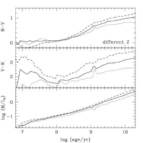
Figure 1: Evolution of the $B\!-\!V$ and $V\!-\!K$ colours and stellar mass-to-light ratio $M/L_{V}$ of simple stellar populations for different metallicities, $Z=0.004$ (dotted line), $Z=Z_{\sun}=0.02$ (solid line) and $Z=0.05$ (dashed line), for the standard model of Section 3. All models have the Chabrier (2003b) IMF truncated at $0.1\,M_{\odot}$ and $100\,M_{\odot}$ (see equation 2).

3.1 Influence of the adjustable parameters

The spectral evolution of an SSP depends primarily on the assumed metallicity, stellar evolution prescription, stellar spectral library and IMF. Here, we illustrate the influence of these adjustable parameters on the evolution of the $B\!-\!V$ and $V\!-\!K$ colours and stellar mass-to-visual light ratio $M/L_{V}$ of an SSP. Optical and near-infrared colours reflect the relative contributions of hot and cool stars to the integrated light, while the stellar mass-to-light ratio reflects the absolute magnitude scale of the model. When computing $M/L_{V}$, we account for the mass lost by evolved stars to the interstellar medium in the form of winds, planetary nebulae and supernova ejecta.

Fig. 1 shows the evolution of the $B\!-\!V$ and $V\!-\!K$ colours and $M/L_{V}$ for three different metallicities, $Z=0.004$, $Z=Z_{\sun}=0.02$ and $Z=0.05$, for our standard SSP model. The irregularities in the photometric evolution arise both from the discrete sampling of initial stellar masses in the track library and from ‘phase’ transitions in stellar evolution. For example, the evolution of low-mass stars through the helium flash causes a characteristic feature in all properties in Fig. 1 at ages near $10^{9}\,$yr. At fixed age, the main effect of increasing metallicity is to redden the colours and increase $M/L_{V}$. The reason for this is that, at fixed initial stellar mass, lowering metallicity causes stars to evolve at higher effective temperatures and higher luminosities (Schaller et al. 1992; Fagotto et al. 1994a, Girardi et al. 2000). Another noticeable effect of varying $Z$ is to change the relative numbers of red and blue supergiants. The evolution of the $B\!-\!V$ colour at early ages in Fig. 1 shows that the signature of red supergiants in the colour evolution of an SSP depends crucially on metallicity (see also Cerviño & Mas-Hesse 1994). We note that increasing metallicity at fixed age has a similar effect as increasing age at fixed metallicity, which leads to the well-known age-metallicity degeneracy.

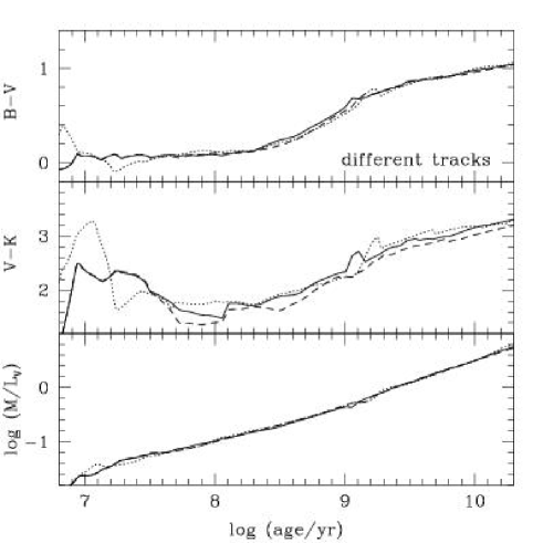
Figure 2: Evolution of the $B\!-\!V$ and $V\!-\!K$ colours and stellar mass-to-light ratio $M/L_{V}$ of simple stellar populations of solar metallicity computed using the Geneva (dotted line), Padova 1994 (standard model; solid line) and Padova 2000 (dashed line) stellar evolution prescriptions and the STELIB/BaSeL 3.1 spectral calibration. All models have the Chabrier (2003b) IMF truncated at $0.1\,M_{\odot}$ and $100\,M_{\odot}$ (see equation 2).

In Fig. 2, we illustrate the influence of the stellar evolution prescription on the predicted photometric evolution of an SSP for fixed (solar) metallicity and fixed (STELIB/BaSeL 3.1) spectral calibration. We show models computed using the Padova 1994, the Geneva and the Padova 2000 track libraries (Section 2.1). The largest difference between the Padova 1994 and Geneva prescriptions arises at early ages and results from the larger number of evolved, blue massive (Wolf-Rayet) stars in the Padova models than in the Geneva models (see fig. 2b of Charlot 1996). Also, since the minimum mass for quiet helium ignition is lower in the Geneva model than in the Padova 1994 model ($1.9\,\mbox{$M_{\odot}$}$ versus $2.2\,\mbox{$M_{\odot}$}$), the photometric signature of the helium flash occurs at slightly later ages in the Geneva model in Fig. 2. Differences between the Padova 1994 and Padova 2000 track libraries pertain only to stars less massive than $7\,\mbox{$M_{\odot}$}$, with turnoff ages greater than about $5\times 10^{7}\,$yr (Section 2.1). In the Padova 2000 model, the finer resolution in initial stellar mass around $2.0\,\mbox{$M_{\odot}$}$ makes the evolution through the helium flash much smoother than in the Padova 1994 model. At late ages, the $V\!-\!K$ colour is significantly bluer in the Padova 2000 model than in the Padova 1994 model. The reason for this is that the red giant branch is 50 to 200 K warmer (from bottom to tip) in the Padova 2000 tracks than in the Padova 1994 tracks. As a result, the integrated $V\!-\!K$ colour of a solar-metallicity SSP in the Padova 2000 model reaches values typical of old elliptical galaxies ($\mbox{$V\!-\!K$}\sim 3.0$–3.3 along the colour-magnitude relation; Bower, Lucey & Ellis 1992) only at ages 15–20 Gyr. Since this is older than currently favored estimates of the age of the Universe, and since the giant-branch temperature in the Padova 2000 tracks has not been tested against observational calibrations (e.g. Frogel, Persson & Cohen 1981), we have adopted here the Padova 1994 library rather than the Padova 2000 library in our standard model (see above).

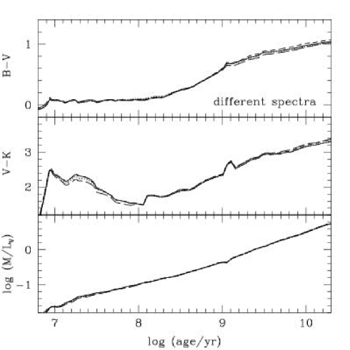
Figure 3: Evolution of the $B\!-\!V$ and $V\!-\!K$ colours and stellar mass-to-light ratio $M/L_{V}$ of simple stellar populations of solar metallicity computed using the Padova 1994 stellar evolution prescription and the BaSeL 3.1 (dotted line), STELIB/BaSeL 1.0 (short-dashed line), STELIB/BaSeL 3.1 (standard model; solid line) and Pickles (long-dashed line) spectral calibrations. All models have the Chabrier (2003b) IMF truncated at $0.1\,M_{\odot}$ and $100\,M_{\odot}$ (see equation 2).

We now consider the influence of the spectral calibration on the photometric evolution of an SSP for fixed (solar) metallicity and fixed (Padova 1994) stellar evolution prescription. In Fig. 3, we compare the results obtained with four different spectral libraries: the STELIB/BaSeL 3.1 library (standard model); the BaSeL 3.1 library; the STELIB/BaSeL 1.0 library; and the Pickles library (recall that, at solar metallicity, the BaSeL 3.1 library is identical to the BaSeL 2.2 library; Section 2.2.1). Fig. 3 shows that the differences between these spectral calibrations have only a weak influence on the predicted photometric evolution of an SSP. The good agreement between the STELIB/BaSeL 3.1, the BaSeL 3.1 and the Pickles calibrations follows in part from the consistent colour-temperature scale of the three libraries. Also the empirical corrections applied by Lejeune et al. (1997) and Westera et al. (2002) to the BaSeL 1.0 spectra, illustrated by the differences between the STELIB/BaSeL 3.1 and STELIB/BaSeL 1.0 models in Fig. 3, imply changes of at most a few hundredths of a magnitude in the evolution of the $B\!-\!V$ and $V\!-\!K$ colours. It is important to note that the spectral calibration has a stronger influence on observable quantities which are more sensitive than integrated colours to the details of the stellar luminosity function, such as colour-magnitude diagrams (Section 3.3) and surface brightness fluctuations (Liu et al., 2000). Fig. 8 of Liu et al. (2000) shows that, for example, the observed near-infrared surface brightness fluctuations of nearby galaxies clearly favor the BaSeL 2.2/3.1 spectral calibration over the BaSeL 1.0 one.

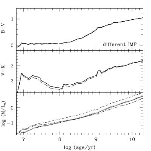
Figure 4: Evolution of the $B\!-\!V$ and $V\!-\!K$ colours and stellar mass-to-light ratio $M/L_{V}$ of simple stellar populations of solar metallicity computed using the Padova 1994 stellar evolution prescription and the STELIB/BaSeL 3.1 spectral calibration, for different IMFs: Chabrier (2003b, standard model; solid line; see equation 2), Kroupa (2001, dotted line), Salpeter (1955, short-dashed line) and Scalo (1998, long-dashed line). All IMFs are truncated at $0.1\,M_{\odot}$ and $100\,M_{\odot}$.

It is also of interest to examine the influence of the IMF on the photometric evolution of an SSP for fixed (solar) metallicity, fixed (Padova 1994) stellar evolution prescription and fixed (STELIB/BaSeL 3.1) spectral calibration. Fig. 4 shows the evolution of the $B\!-\!V$ and $V\!-\!K$ colours and $M/L_{V}$ for four different IMFs: Chabrier (2003b, see equation 2 above), Kroupa (2001, universal IMF), Salpeter (1955) and Scalo (1998). In all cases, the IMF is truncated at $0.1\,M_{\odot}$ and $100\,M_{\odot}$. The evolution of the $B\!-\!V$ colour does not depend sensitively on the IMF, because the optical light is dominated at any age by stars near the turnoff. The $V\!-\!K$ colour is slightly more sensitive to the relative weights of stars of different masses along the isochrone, especially at ages less than about $10^{9}\,$yr, when the mass of the most evolved stars differs significantly from the turnoff mass. The $M/L_{V}$ ratio is far more sensitive to the shape of the IMF, especially near the low-mass end that determines the fraction of the total mass of the stellar population locked into faint, slowly evolving stars. For reference, the fraction of mass returned to the ISM by evolved stars at the age of $10\,$Gyr is 31, 44, 46, and 48 per cent for the Salpeter, the Scalo, the Kroupa and the Chabrier IMFs, respectively.

3.2 Comparison with previous work

Most current population synthesis models rely on readily available computations of stellar evolutionary tracks and stellar atmospheres, such as those mentioned in Section 2.1 and Section 2.2.1 above. In general, however, publically available stellar evolutionary tracks do not include the uncertain evolution of stars beyond the early-AGB phase. Also, the widely used model atmospheres of Kurucz (1992, and other releases) do not include spectra of stars outside the temperature range $3500\,{\rm K}\leq T_{\rm eff}\leq 50,000\,$K. We therefore expect differences between our model and previous work to originate mainly from our observationally motivated prescription for TP-AGB stars, the spectral calibration of very hot and very cool (giant) stars and the adoption of a new library of observed stellar spectra at various metallicities.

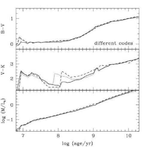
Figure 5: Evolution of the $B\!-\!V$ and $V\!-\!K$ colours and stellar mass-to-light ratio $M/L_{V}$ of simple stellar populations of solar metallicity computed using our model (with the Padova 1994 stellar evolution prescription and the STELIB/BaSeL 2.2 spectral calibration; solid line), the Fioc & Rocca-Volmerange (1997) PÉGASE version 2.0 model (dotted line) and the Girardi et al. (2002) model (dashed line). All models have the Kroupa (2001) present-day IMF truncated at $0.01\,M_{\odot}$ and $100\,M_{\odot}$.

In Fig. 5, we compare the evolution of the $B\!-\!V$ and $V\!-\!K$ colours and the mass-to-visual light ratio $M/L_{V}$ of a solar-metallicity SSP predicted by our model with those predicted by two publically available population synthesis codes: the PÉGASE model (Fioc & Rocca-Volmerange 1997; version 2.0) and the Girardi et al. (2002) model. For practical reasons, we adopt in all models the same IMF as in Girardi et al. (2002), i.e., the Kroupa (2001) present-day IMF truncated at $0.01\,\mbox{$M_{\odot}$}$ and $100\,\mbox{$M_{\odot}$}$. Also, for the purpose of this comparison, we compute our model using the Padova 1994 stellar evolution prescription and the STELIB/BaSeL 2.2 spectral calibration (which is identical to the BaSeL 3.1 calibration for solar metallicity; Section 2.2.1).

The PÉGASE model shows good general agreement with our model in Fig. 5. There are marked discrepancies at ages around $10^{7}\,$yr, where the PÉGASE model is redder in $B\!-\!V$ but bluer in $V\!-\!K$ than our model, and at ages around $10^{8}\,$yr, where it is nearly a magnitude redder in $V\!-\!K$. General agreement is expected because the PÉGASE model relies on the same Padova 1994 tracks as used in our model to describe the evolution of stars up to the end of the early-AGB and on the same BaSeL 2.2 spectral calibration. The discrepancy at early ages arises from a difference in the spectral calibration of stars hotter than 50,000 K. In the PÉGASE model, the spectra of these stars are taken from Clegg & Middlemass (1987), while in our model, they are taken from the more recent computations of Rauch (2002). The discrepancy in the $V\!-\!K$ colour at ages around $10^{8}\,$yr arises from a different prescription for TP-AGB evolution. Fioc & Rocca-Volmerange (1997) use ‘typical’ TP-AGB luminosities and evolutionary time-scales from Groenewegen & de Jong (1993), while in our model, the evolution through this phase and its spectral calibration are more refined (Section 2.1 and Section 2.2).

The Girardi et al. (2002) model in Fig. 5 relies on the Padova 2000 stellar evolutionary tracks and on model atmospheres by Castelli, Gratton & Kurucz (1997) and Fluks et al. (1994). These model atmospheres do not include any empirical colour-temperature correction and are akin to the Kurucz (1995, private communication to R. Buser) and Fluks et al. (1994) spectra included in the BaSeL 1.0 library. It is interesting to note that, when combined with these purely theoretical model atmospheres, the Padova 2000 evolutionary tracks, in which the giant branch is relatively warm (Section 3.1), produce $B\!-\!V$ and $V\!-\!K$ colours in good agreement with those predicted both by the PÉGASE model and by our model at late ages. At ages less than $10^{7}\,$yr and around $10^{8}\,$yr, the Girardi et al. (2002) model deviates from our model in a similar way as the PÉGASE model. The discrepancy at early ages is caused again by a different treatment of stars hotter than 50,000 K, which Girardi et al. (2002) describe as simple blackbody spectra. The discrepancy at ages $10^{8}$–$10^{9}\,$yr follows primarily from the treatment of TP-AGB evolution, which is based on a semi-analytic prescription by Girardi & Bertelli (1998) in the Girardi et al. (2002) model. It is worth recalling that our prescription for TP-AGB evolution has been tested successfully against observed optical and near-infrared surface brightness fluctuations of nearby star clusters and galaxies (Section 2).

3.3 Comparison with observations of star clusters

3.3.1 Colour-magnitude diagrams

Table 4: Star cluster data.

Cluster	Alias	$(m-M)_{0}$	$E(\mbox{$B\!-\!V$})$	$\hbox{\rm[Fe/H]}_{\rm obs}$	$Z_{\rm mod}$	$\hbox{\rm[Fe/H]}_{\rm mod}$	$t_{\rm mod}$/Gyr	References
NGC6397		12.31	0.18	$-1.94$	0.0004	$-1.65$	14	1, 2, 3
NGC6809	M55	13.82	0.07	$-1.80$	0.0004	$-1.65$	13	4, 5
NGC5139	$\omega$Cen	13.92	0.12	$-1.62$	0.0004	$-1.65$	13	4, 5
NGC104	47Tuc	13.32	0.05	$-0.71$	0.004	$-0.64$	13	4, 6
NGC6528		14.45	0.52	$-0.35$	0.008	$-0.33$	13	7, 8
NGC6553		13.60	0.70	$-0.35$	0.008	$-0.33$	13	7, 8, 9
NGC2682	M67	9.50	0.06	$+0.01$	0.02	$+0.09$	4	10, 11, 12, 13, 14
Hyades		3.40	0.00	$+0.15$	0.02	$+0.09$	0.7	15, 16, 17, 18

(1) King et al. (1998); (2) D’Antona (1999); (3) Kaluzny (1997); (4) Rosenberg et al. (2000a); (5) Rosenberg et al. (2000b); (6) Kaluzny et al. (1998); (7) Bruzual et al. (1997); (8) Ortolani et al. (1995); (9) Guarnieri et al. (1998); (10) Eggen & Sandage (1964); (11) Gilliland et al. (1991); (12) Janes & Smith (1984); (13) Montgomery, Marschall & Janes (1993); (14) Racine (1971); (15) Micela et al. (1988); (16) Upgren (1974); (17) Upgren & Weis (1977); (18) Mermilliod (2000).

To establish the reliability of our model, it is important to examine the accuracy to which it can reproduce observed colour-(absolute) magnitude diagrams (CMDs) of star clusters of different ages and metallicities. Table 4 contains a list of star clusters for which extensive data are available from the literature. The clusters are listed in order of increasing [Fe/H]. For each cluster, we list the distance modulus $(m-M)_{0}$ and the colour excess $E(\mbox{$B\!-\!V$})$ from the same references as for the stellar photometry. The reddening-corrected CMDs of these clusters are presented in Figs 6 and 7, where we show the absolute $V$ magnitude as a function of various available optical and infrared colours. Superimposed on the data in each frame are four isochrones. The red isochrones are computed using the Padova 1994 tracks, while the black isochrones are computed using the Padova 2000 tracks. In each case, the dashed and solid isochrones are computed using the BaSeL 1.0 and BaSeL 3.1 spectral calibrations, respectively. The isochrones were selected by adopting the available model metallicity closest to the cluster [Fe/H] value and then choosing the age that provided the best agreement with the data. Age and metallicity are the same for all the isochrones for each cluster. Columns 6, 7 and 8 of Table 4 list the metallicity $Z_{\rm mod}$, the corresponding $\hbox{\rm[Fe/H]}_{\rm mod}$ and the age $t_{\rm mod}$ adopted for each cluster. The listed ages are in good agreement with previous determinations.

Fig. 6 shows the CMDs of two Galactic open clusters of near-solar metallicity in various photometric bands: the young Hyades cluster and the intermediate-age M67 cluster. For clarity, stars near and past the turnoff are plotted as large symbols. In the case of the Hyades, the 700 Myr Padova 1994/BaSeL 3.1 isochrone reproduces well the upper main sequence, the turnoff and the core-He burning phase in all $UBVIR$ bands. For M67, the 4 Gyr Padova 1994/BaSeL 3.1 isochrone fits remarkably well the upper main sequence, the subgiant branch, the red giant branch, the core-He burning clump and the AGB in all bands. For both clusters, the models predict slightly bluer $UBV$ colours than observed on the lower main sequence. The offset is smaller in $R-I$ for the Hyades and in $V-R$ for M67, but the data are sparse in both cases. It is worth noting that, for $M_{V}>10$, the BaSeL 3.1 spectral calibration provides better agreement with the data than the BaSeL 1.0 calibration. Lower-main sequence stars, in any case, contribute negligibly to the integrated light of a star cluster or a galaxy. At the age of the Hyades, the Padova 1994 and 2000 isochrones differ very little, as they rely on the same stellar evolution prescription for massive stars (Section 2.1). At the age of M67, the Padova 2000 isochrone tends to predict stars bluer and brighter than the Padova 1994 isochrone near the tip of the red giant branch. As seen in Section 3.1 above, this small but significant difference has a noticeable influence on integrated-light properties (see also below).

Fig. 7 shows the optical-infrared CMDs of six old Galactic globular clusters of different metallicities. NGC 6397 is the most metal-poor cluster in our sample, with $\hbox{\rm[Fe/H]}=-1.94$ (Table 4). Fig. 7(a) shows that models with $Z=0.0004$ ($\hbox{\rm[Fe/H]}_{\rm mod}\approx-1.65$) at an age of 14 Gyr provide excellent fits to the Hubble Space Telescope (HST) data for this cluster, all the way from the main sequence, to the red giant branch, to the AGB and to the white-dwarf cooling sequence. The models, however, do not fully reproduce the observed extension of the blue horizontal branch (see also below). This problem persists even if the age of the isochrones is increased. For this cluster, the Padova 2000/BaSeL 3.1 isochrone appears to fit the shape of the horizontal branch and the main sequence near $M_{V}=8$ marginally better than the Padova 1994/BaSeL 3.1 isochrone. Ground-based data for the other two low-metallicity clusters in our sample, NGC 6809 ($\hbox{\rm[Fe/H]}=-1.80$) and NGC 5139 ($\hbox{\rm[Fe/H]}=-1.62$), are also reproduced reasonably well by the $\hbox{\rm[Fe/H]}_{\rm mod}=-1.65$ isochrones at an age of 13 Gyr (Figs 7b and 7c). As in the case of NGC 6397, the models do not reproduce the full extension of the blue horizontal branch. This suggests that this mismatch is not purely a metallicity effect and that the evolution of these stars, or their spectral calibration, or both, may have to be revised in the models. It is worth pointing out that the BaSeL 3.1 spectral calibration provides a better fit of the upper red-giant stars than the BaSeL 1.0 calibrations at these low metallicities.

The CMD of the intermediate-metallicity cluster NGC 104 ($\hbox{\rm[Fe/H]}=-0.71$) is well reproduced by the Padova 1994/BaSeL 3.1 model with $\hbox{\rm[Fe/H]}_{\rm mod}=-0.64$ at the age of 13 Gyr (Fig. 7d). This age should be regarded only as indicative, as the stars in NGC 104 are known to be overabundant in $\alpha$ elements relative to the solar composition, whereas the model has scaled-solar abundances (see Vazdekis et al. 2001 for a more detailed analysis). The NGC 6528 and NGC 6553 clusters of the Galactic bulge in Figs. 7e–7g are more metal-rich, with $\hbox{\rm[Fe/H]}=-0.35$. The Padova 1994/BaSeL 3.1 model with $\hbox{\rm[Fe/H]}_{\rm mod}=-0.41$ provides good fits to the CMDs of these clusters at the age of 13 Gyr. For both clusters, the position of the core-He burning clump and the extension of the red giant branch toward red $V-I$ and $V\!-\!K$ colours are especially well accounted for. As in the case of M67 (Fig. 6), the Padova 2000 isochrones tend to predict stars bluer and brighter than the Padova 1994 isochrones on the upper red giant branch, providing a slightly worse fit to the observations. Also, as is the case at other metallicities, the BaSeL 3.1 spectral calibration provides a better fit of the upper red-giant stars than the BaSeL 1.0 calibration.

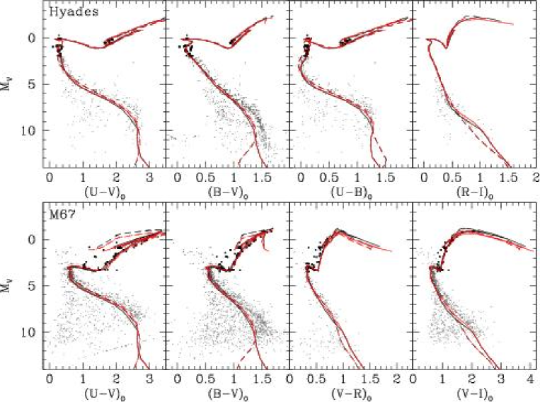
Figure 6: Comparison of model isochrones with observed colour-magnitude diagrams of the Hyades and M67 Galactic open clusters in various photometric bands. For clarity, stars near and past the turnoff are plotted as large symbols. For each cluster, the adopted distance modulus and colour excess are listed in Table 4 along with the sources of the stellar photometry. Each panel contains four isochrones: the red isochrones are computed using the Padova 1994 tracks, while the black isochrones are computed using the Padova 2000 tracks. In each case, the dashed and solid isochrones are computed using the BaSeL 1.0 and BaSeL 3.1 spectral calibrations, respectively. All isochrones pertaining to a given cluster have fixed age and metallicity (see Table 4).

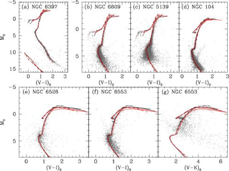
Figure 7: Comparison of model isochrones with observed colour-magnitude diagrams of six old Galactic globular clusters. For each cluster, the adopted distance modulus and colour excess are listed in Table 4 along with the sources of the stellar photometry. Each panel contains four isochrones: the red isochrones are computed using the Padova 1994 tracks, while the black isochrones are computed using the Padova 2000 tracks. In each case, the dashed and solid isochrones are computed using the BaSeL 1.0 and BaSeL 3.1 spectral calibrations, respectively. All isochrones pertaining to a given cluster have fixed age and metallicity (see Table 4).

Overall, Figs 6 and 7 show that our model provides excellent fits to observed CMDs of star clusters of different ages and metallicities in a wide range of photometric bands. The data tend to favor the combination of the Padova 1994 stellar evolution prescription with the BaSeL 3.1 spectral calibration. This justifies our adoption of this combination in our standard model.

3.3.2 Integrated colours

We must also check that our model can reproduce the integrated colours of star clusters of various ages and metallicities, which are sensitive to the numbers of stars populating different phases along the isochrones. Figs 8(a) and 8(b) show the integrated, reddening-corrected $U\!-\!B$, $B\!-\!V$ and $V\!-\!K$ colours of LMC clusters in various age ranges, according to the classification scheme of Searle, Wilkinson & Bagnuolo (1980,  hereafter SWB). Also shown as error bars are the colours of young star clusters in the merger remnant galaxy NGC 7252 from Miller et al. (1997) and Maraston et al. (2001). The solid line shows the evolution of our standard SSP model for $Z=0.4Z_{\odot}$, at ages ranging from a few Myr at the blue end of the line to 13 Gyr at the red end of the line. The scatter in cluster colours in Figs 8(a) and 8(b) is intrinsic (typical observational errors are indicated in each panel). It is largest in $V\!-\!K$ colour (Fig. 8b) but is also present, to a lesser extent, in $U\!-\!B$ and $B\!-\!V$ colours (Fig. 8a). This scatter cannot be accounted for by metallicity variations. The age-metallicity degeneracy implies that the evolution of SSPs with various metallicities are similar to that of the $Z=0.4Z_{\odot}$ model in these colour-colour diagrams. For reference, the heavy dashed line in Figs 8(a) and 8(b) shows the colours of the standard SSP model of Section 3 for the metallicity $Z=Z_{\odot}$ at ages from 100 Myr to 1 Gyr. The scatter in the observed integrated colours of star clusters is most likely caused by stochastic fluctuations in the numbers of stars populating different evolutionary stages.

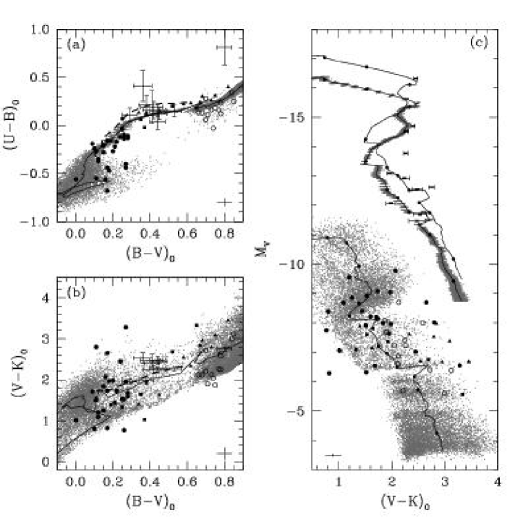
Figure 8: (a) $U\!-\!B$ versus $B\!-\!V$ and (b) $V\!-\!K$ versus $B\!-\!V$ integrated colours of star clusters. The different symbols represent LMC globular clusters in various age ranges according to the SWB classification scheme (classes I–III: filled circles; class IV: squares; class V: triangles; classes VI–VII: open circles). The $U\!-\!B$ and $B\!-\!V$ colours are from van den Bergh (1981) and the $V\!-\!K$ colours from Persson et al. (1983). The points with error bars are young star clusters in the merger remnant galaxy NGC 7252 (Miller et al. 1997; Maraston et al. 2001). The solid line shows the evolution of the standard SSP model of Section 3 for the metallicity $Z=0.4Z_{\odot}$ at ages from a few Myr to 13 Gyr. The small dots show the results of 22,000 stochastic realizations of the integrated colours of clusters of mass $2\times 10^{4}\,M_{\odot}$ at ages between $10^{5}$ and 13 Gyr, for the same metallicity and IMF as for this SSP model. The heavy dashed line shows the colours of the standard SSP model of Section 3 for the metallicity $Z=Z_{\odot}$ at ages from 100 Myr to 1 Gyr. (c) Absolute magnitude $M_{V}$ versus $V\!-\!K$ colour. The data are the same as in (a) and (b). Three models show the evolution of, from bottom to top, a $2\times 10^{4}\,M_{\odot}$ SSP with metallicity $Z=0.4Z_{\odot}$, a $3\times 10^{6}\,M_{\odot}$ SSP with metallicity $Z=Z_{\odot}$ and a $6\times 10^{6}\,M_{\odot}$ SSP with metallicity $Z=Z_{\odot}$. Small circles indicate the positions of the models at the ages 6, 7, 10, 100, 400 and 500 Myr and 1, 1.4, 2 and 10 Gyr (these marks can be used to roughly date the clusters). Stochastic realizations of integrated colours are shown only for the two least massive models, as the predicted scatter is small for the most massive one. Typical observational error bars are indicated at the bottom of each panel.

We illustrate this by generating random realizations of integrated cluster colours using a Monte Carlo technique pioneered by Barbaro & Bertelli (1977) (see also Chiosi, Bertelli & Bressan 1988; Girardi et al. 1995; Santos & Frogel 1997; Bruzual 2002; Cerviño et al. 2001; Cerviño et al. 2002). For a given cluster age, we draw stars randomly from the IMF of equation (2) and place them in their evolutionary phase along the isochrone at that age, until a given cluster mass is reached. The small dots in Figs 8(a) and 8(b) show the results of 22,000 such realizations for clusters of mass $2\times 10^{4}\,M_{\odot}$ and metallicity $Z=0.4Z_{\odot}$, at ages between $10^{5}$ and 13 Gyr (see Bruzual 2002 for more detail). It is clear from these figures that the models can account for the full observed ranges of integrated cluster colours, including the scatter of nearly 2 mag in $V\!-\!K$ colour. The reason for this is that the $V\!-\!K$ colour is highly sensitive to the small number of bright stars populating the upper giant branch. Fluctuations are smaller in the $U\!-\!B$ and $B\!-\!V$ colours, which are dominated by the more numerous main-sequence stars. The predicted scatter would be smaller in all colours for clusters more massive than $2\times 10^{4}\,M_{\odot}$, as the number of stars in any evolutionary stage would then be larger (Bruzual 2002; Cerviño et al. 2002).

To further illustrate the relation between cluster mass and scatter in integrated colours, we plot in Fig. 8(c) the absolute $V$ magnitude as a function of $V\!-\!K$ colour for the same clusters as in Figs 8(a) and 8(b). The three models shown correspond to the evolution of, from bottom to top, a $2\times 10^{4}\,M_{\odot}$ SSP with metallicity $Z=0.4Z_{\odot}$, a $3\times 10^{6}\,M_{\odot}$ SSP with metallicity $Z=Z_{\odot}$ and a $6\times 10^{6}\,M_{\odot}$ SSP with metallicity $Z=Z_{\odot}$. We show stochastic realizations of integrated colours only for the two least massive models, as the predicted scatter is small for the most massive one. As in Figs 8(a) and 8(b), random realizations at various ages of $2\times 10^{4}\,M_{\odot}$ clusters with metallicity $Z=0.4Z_{\odot}$ can account for the full observed range of LMC cluster properties in this diagram. The NGC 7252 clusters are consistent with being very young (100–800 Myr) and massive ($10^{6}-10^{7}\,M_{\odot}$) at solar metallicity, in agreement with the results of Schweizer & Seitzer (1998).

Our models, therefore, reproduce remarkably well the full observed ranges of integrated colours and absolute magnitudes of star clusters or various ages and metallicities. It is worth pointing out that, because of the stochastic nature of the integrated-light properties of star clusters, single clusters may not be taken as reference standards of simple stellar populations of specific age and metallicity.

4 Spectral evolution

We now turn to the predictions of our models for the spectral evolution of stellar populations. In Section 4.1 below, we begin by describing the canonical evolution of the spectral energy distribution of a simple stellar population. We also illustrate the influence of metallicity on the spectra. Then, in Section 4.2, we compare our model with observed galaxy spectra extracted from the SDSS EDR. Section 4.3 presents a more detailed comparison of the predicted and observed strengths of several absorption-line indices.

4.1 Simple stellar population

Fig. 9 shows the spectral energy distribution of the standard SSP model of Section 3 at various ages and for solar metallicity. As is possible for this metallicity (Section 2.2.2), we have extended the STELIB/BaSeL 3.1 library blueward of 3200 Å and redward of 9500 Å using the Pickles medium-resolution library (Section 2.2.3). In Fig. 9, therefore, the model includes libraries of observed stellar spectra across the whole wavelength range from 1205 Å to 2.5 $\mu$m.

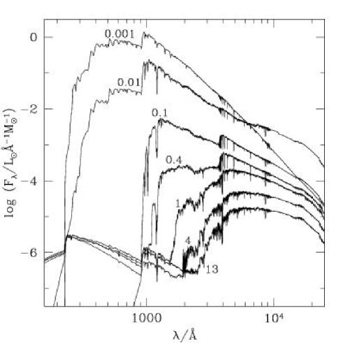
Figure 9: Spectral evolution of the standard SSP model of Section 3 for the solar metallicity. The STELIB/BaSeL 3.1 spectra have been extended blueward of 3200 Å and redward of 9500 Å using the Pickles medium-resolution library. Ages are indicated next to the spectra (in Gyr).

The spectral evolution of an SSP may be understood in terms of the evolution of its stellar content. At $10^{6}$ yr, the spectrum in Fig. 9 is entirely dominated by short-lived, young massive stars with strong ultraviolet emission on the upper main sequence. Around $10^{7}$ yr, the most massive stars leave the main sequence and evolve into red supergiants, causing the ultraviolet light to decline and the near-infrared light to rise. From a few times $10^{8}$ yr to over $10^{9}$ yr, AGB stars maintain a high near-infrared luminosity. The ultraviolet light continues to drop as the turnoff mass decreases on the main sequence. After a few gigayears, red giant stars account for most of the near-infrared light. Then, the accumulation of low-mass, post-AGB stars causes the far-ultraviolet emission to rise until 13 Gyr. The most remarkable feature in Fig. 9 is the nearly unevolving shape of the optical to near-infrared spectrum at ages from 4 to 13 Gyr. The reason for this is that low-mass stars evolve within a narrow temperature range all the way from the main sequence to the end of the AGB.

The scale of Fig. 9 is not optimal to fully appreciate the spectral resolution of the model. However, some variations can be noticed in the strengths of prominent absorption lines. At ages between 0.1 and 1 Gyr, for example, there is a marked strengthening of all Balmer lines from H$\alpha$ at 6563 Å to the Balmer continuum limit at 3646 Å. This characteristic signature of a prominent population of late-B to early-F stars is, in fact, a standard diagnostic of recent bursts of star formation in galaxies (e.g., Couch & Sharples 1987; Poggianti et al. 1999; Kauffmann et al. 2003). It is interesting to note how, over the same age interval, the ‘Balmer break’ (corresponding to the Balmer continuum limit) evolves into the ‘4000 Å break’ (arising from the prominence in cool stars of a large number of metallic lines blueward of 4000 Å). Other prominent absorption features in Fig. 9 include the Mg II resonance doublet near 2798 Å, the Ca II H and K lines at 3933 Å and 3968 Å, and the Ca II triplet at 8498, 8542, and 8662 Å. These features tend to strengthen with age as they are stronger in late-type stars than in early-type stars, whose opacities are dominated by electron scattering. However, the strengths of these features also depend on the abundances of the heavy elements that produce them.

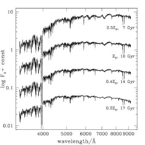
Figure 10: Spectra of the standard SSP model of Section 3 at different ages for different metallicities, as indicated. The prominent metallic features show a clear strengthening from the most metal-poor to the most metal-rich models, even though the shape of the spectral continuum is roughly similar in all models.

Fig. 9 also shows that the strengths of many absorption lines, in contrast to the spectral continuum shape, continue to evolve significantly at ages between 4 and 13 Gyr. Since the strengths of such features are expected to react differently to age and metallicity, they can potentially help us resolve the age-metallicity degeneracy that hampers the interpretation of galaxy spectra (see Section 3.1; Rose 1985; Worthey 1994; Vazdekis 1999). This is illustrated by Fig. 10, in which we show the spectra of SSPs of different ages and metallicities, whose spectral continua have roughly similar shapes. The prominent metallic features in these spectra, such as the Ca II H and K lines, the many Fe and Mg lines between 4500 and 5700 Å, and several TiO, H₂O and O₂ molecular absorption features redward of 6000 Å, show a clear strengthening from the most metal-poor to the most metal-rich stellar populations. As we shall see in Sections 4.2 and 4.3 below, the analysis of these features in observed galaxy spectra provide useful constraints on the metallicities, and in turn on the ages, of the stellar populations that dominate the emission.

4.2 Interpretation of galaxy spectra

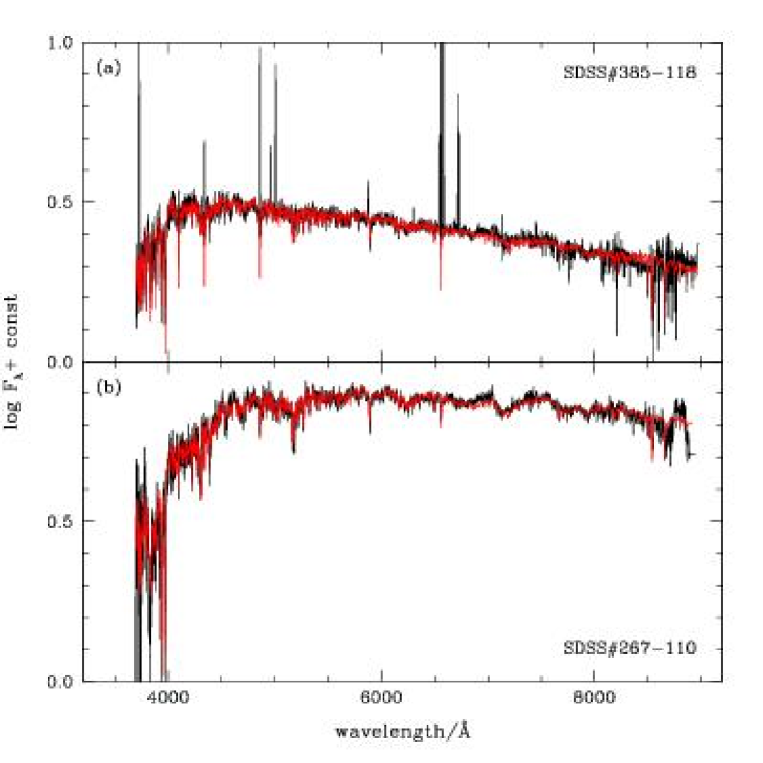
Figure 11: Model fits (red spectra) of two galaxies extracted from the SDSS Early Data Release (black spectra). The fits were derived using the optimized data compression algorithm of Heavens, Jimenez & Lahav (2000), as described in the text. The emission lines of SDSS 385–118 were removed to perform the fit.

We now exemplify how our model can be used to interpret observed galaxy spectra. The observational sample we consider is the Early Data Release of the Sloan Digital Sky Survey (Stoughton et al. 2002; see Section 1). This survey will obtain $u$, $g$, $r$, $i$, and $z$ photometry of almost a quarter of the sky and spectra of at least 700,000 objects. The ‘main galaxy sample’ of the EDR includes the spectra of 32,949 galaxies with $r$-band Petrosian magnitudes brighter than 17.77 after correction for foreground Galactic extinction (Strauss et al., 2002). The spectra are flux- and wavelength-calibrated, with 4096 pixels from 3800 Å to 9200 Å at resolving power $\lambda/\Delta\lambda\approx 1800$. This is similar to the resolution of our model in the wavelength range from 3200 Å to 9500 Å. The SDSS spectra are acquired using 3-arcsecond diameter fibres that are positioned as close as possible to the centres of the target galaxies. For the purpose of first illustration, we select SDSS spectra of two representative galaxies of different types according to their 4000 Å discontinuities. We adopt here the 4000 Å discontinuity index defined by Balogh et al. (1999) as the ratio of the average flux density $F_{\nu}$ in the narrow bands 3850–3950 Å and 4000–4100 Å. The original definition of this index by Bruzual (1983) uses wider bands (3750–3950 Å and 4050–4250 Å), and hence, it is more sensitive to reddening effects. We select two spectra with median signal-to-noise ratios per pixel larger than 30 and with discontinuity indices near opposite ends of the sample distribution, $D_{n}(4000)=1.26$ (SDSS 385–118) and $D_{n}(4000)=1.92$ (SDSS 267–110). The galaxies have measured line-of-sight velocity dispersions $\hbox{$\sigma_{V}$}\approx 70~{}\hbox{${\rm km}\,{\rm s}^{-1}$}$ and $130~{}\hbox{${\rm km}\,{\rm s}^{-1}$}$, respectively. The spectra are corrected for foreground Galactic extinction using the reddening maps of Schlegel, Finkbeiner & Davis (1998) and the extinction curve of Fitzpatrick (1999).

To interpret these spectra with our model, we use MOPED, the optimized data compression algorithm of Heavens, Jimenez & Lahav (2000). In this approach, galaxy spectra are compressed into a reduced number of linear combinations connected to physical parameters such as age, star formation history, metallicity and dust content. The linear combinations contain as much information about the parameters as the original spectra. There are several advantages to this method. First, it allows one to explore a wide range of star formation histories, chemical enrichment histories and dust contents by choosing appropriate parametrizations (Reichardt, Jimenez & Heavens, 2001). Second, it allows one to estimate the errors on derived physical parameters. And third, it is extremely fast and hence efficient to interpret large numbers of galaxy spectra. Our model has already been combined with the MOPED algorithm to interpret SDSS EDR spectra (Mathis et al., in preparation). The results presented for the two galaxies considered here are based on a decomposition of the star formation history into six episodes of constant star formation in the age bins 0.0–0.01, 0.01–0.1, 0.1–1.0, 1.0–2.5, 2.5–5 and 5–13 Gyr. The metallicity in each bin can be one of $Z=0.4Z_{\sun}$, $Z_{\sun}$ or $2.5Z_{\sun}$. The attenuation by dust is parametrized using the simple two-component model of Charlot & Fall (2000, see Section 5 below). The effective attenuation optical depth affecting stars younger than 0.01 Gyr can be $\hbox{$\hat{\tau}_{V}$}=0.0$, 0.1, 0.5, 1, 1.5, 2 or 3, while that affecting older stars is $\mu\hbox{$\hat{\tau}_{V}$}$, with $\mu=0.0$, 0.1, 0.3, 0.5 or 1 (see equation 6 below; we are grateful to H. Mathis for providing us with the results of these fits).

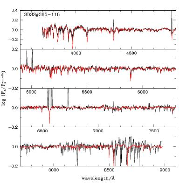
Figure 12: Detailed comparison of ‘high-pass’ spectra for the same model (in red) of SDSS galaxy 385–118 (in black) as in Fig. 11(a). The high-pass spectra were obtained by smoothing the original spectra using a top-hat function of width 200 Å and then dividing the original spectra by the smoothed spectra.

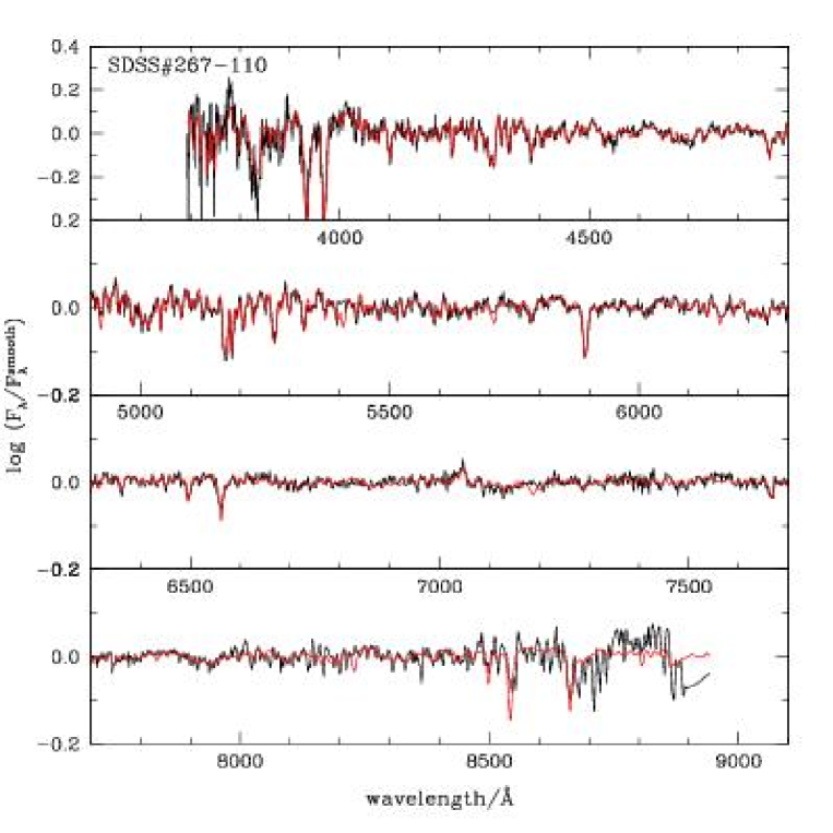
Figure 13: Detailed comparison of ‘high-pass’ spectra for the same model (in red) of SDSS galaxy 267–110 (in black) as in Fig. 11(b). The high-pass spectra were obtained by smoothing the original spectra using a top-hat function of width 200 Å and then dividing the original spectra by the smoothed spectra.

Fig. 11 shows the resulting spectral fits of SDSS 385–118 and SDSS 267–110. Figs 12 and 13 show details of the ‘high-pass’ spectra of the fitted models and observed galaxies (note that we display the emission lines of SDSS 385–118 in Figs 11a and 12, even though these were removed to perform the fit). The high-pass spectra were obtained by smoothing the original spectra using a top-hat function of width 200 Å and then dividing the original spectra by the smoothed spectra (see Baldry et al. 2002). The model reproduces the main stellar absorption features of both galaxies extremely well. In particular, in the spectrum of SDSS 385–118, the absorption wings of Balmer lines are well fitted up to high orders in the series. With such an accuracy, the model can be used reliably to measure the contamination of Balmer emission lines by underlying stellar absorption in galaxies (see Tremonti 2003). This is especially important, for example, to constrain attenuation by dust using the H$\alpha$/H$\beta$ ratio. The spectrum of SDSS 267–110 in Fig. 13 shows no obvious emission lines and exhibits strong stellar absorption features characteristic of old stellar populations. Among the most recognizable features, the Ca II H and K lines, the $G$ band near 4300 Å, the magnesium features near 5100 Å and 5200 Å, the iron features between 5270 Å and 5800 Å, the NaD feature near 5900 Å, and the TiO bands near 6000 Å and 6200 Å are all well reproduced by the model. In Section 4.3 below, we compare in a more quantitative way the strengths of these features in our model with those in the SDSS EDR spectra.

It is of interest to mention the physical parameters of the model fits in Figs 11–13. For SDSS 385–118, the algorithm assigns 91 per cent of the total stellar mass of $\sim 10^{9}M_{\sun}$ to stars with metallicity $Z=0.4Z_{\sun}$ formed between 2.5 and 13 Gyr ago, and the remainder to stars of the same metallicity formed in the last Gyr or so. The galaxy is best fitted with $\mu\hbox{$\hat{\tau}_{V}$}=0.5$. For SDSS 267–110, 50 per cent of the total stellar mass of $\sim 10^{10}M_{\sun}$ is attributed to stars formed 5–13 Gyr ago and the remainder to stars formed 2.5–5 Gyr ago, all with solar metallicity. The dust attenuation optical depth is found to be negligible, with $\hbox{$\hat{\tau}_{V}$}=0$. The total stellar masses quoted here do not include aperture corrections for the light missed by the 3-arcsec diameter fibres. The errors in the derived mass fractions in our various bins are relatively modest, of the order of 20 per cent, for these spectra with high signal-to-noise ratios (Mathis et al., in preparation).

The examples described above illustrate how our model can be used to interpret observed high-resolution spectra of galaxies at wavelength from 3200 Å to 9500 Å in terms of physical parameters such as age, star formation history, chemical enrichment history and dust content.

4.3 Spectral indices

It is important to establish in a more quantitative way the ability of our model to reproduce the strengths of prominent stellar absorption features in observed galaxy spectra. The atomic and molecular features that are most commonly measured in the visible spectra of galaxies are those defined in the extended Lick system (Worthey et al. 1994; Worthey & Ottaviani 1997; Trager et al. 1998; see Section 1). This system includes a total of 25 spectral indices that were defined and calibrated in the spectra of 460 Galactic stars covering the wavelength range from 4000 Å to 6400 Å at a resolution of $\sim 9$ Å FWHM. In the Lick system, an index is defined in terms of a central ‘feature bandpass’ bracketed by two ‘pseudo-continuum bandpasses’. By convention, atomic indices are expressed in angstroms of equivalent width, while molecular indices are expressed in magnitudes.

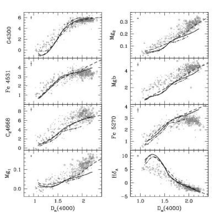
Figure 14: Strengths of G4300, Fe4531, C₂4668, Mg₁, Mg₂, Mgb, Fe5270 and H$\delta_{A}$ as a function of $D_{n}(4000)$ for 543 galaxies with S/N${}_{\rm med}\geq 40$ in the ‘main galaxy sample’ of the SDSS EDR (the median observational error bars are indicated in the upper left corner of each panel). Different symbols correspond to different velocity dispersions (crosses: $\hbox{$\sigma_{V}$}\leq 100~{}\hbox{${\rm km}\,{\rm s}^{-1}$}$; dots: $100<\hbox{$\sigma_{V}$}\leq 250~{}\hbox{${\rm km}\,{\rm s}^{-1}$}$; open circles: $\hbox{$\sigma_{V}$}>250~{}\hbox{${\rm km}\,{\rm s}^{-1}$}$). The lines show the evolution of the standard SSP model of Section 3 for the metallicities $Z=0.008$ (dot-and-dashed line), $Z=0.02$ (solid line) and $Z=0.05$ (dashed line) at ages from $5\times 10^{7}\,$yr to 15 Gyr. The models have 3 Å FWHM spectral resolution, corresponding to a nominal stellar velocity dispersion $\hbox{$\sigma_{V}$}\approx 70~{}\hbox{${\rm km}\,{\rm s}^{-1}$}$ at 5500 Å.

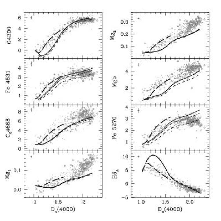
Figure 15: Strengths of G4300, Fe4531, C₂4668, Mg₁, Mg₂, Mgb, Fe5270 and H$\delta_{A}$ as a function of $D_{n}(4000)$ for the same SDSS galaxies as in Fig. 14. The lines show the evolution of the standard SSP model of Section 3 for solar metallicity and for stellar velocity dispersions $\hbox{$\sigma_{V}$}=70~{}\hbox{${\rm km}\,{\rm s}^{-1}$}$ (nominal model velocity dispersion, solid line), 150 ${\rm km}\,{\rm s}^{-1}$ (dot-and-dashed line) and 300 ${\rm km}\,{\rm s}^{-1}$ (dashed line) at ages from $5\times 10^{7}\,$yr to 15 Gyr. The long-dashed line shows the evolution of a model with continuous star formation with a law $\psi(t)\propto\exp\left[-t/({\rm 4\,Gyr)}\right]$, for $Z=Z_{\odot}$ and $\hbox{$\sigma_{V}$}=70~{}\hbox{${\rm km}\,{\rm s}^{-1}$}$.

We compare the Lick index strengths predicted by our model with those measured in SDSS EDR spectra with high signal-to-noise ratios. We do not use here the index strengths included in the SDSS EDR. Instead, we re-measure index strengths in the SDSS spectra in the same way as in the model spectra (we are grateful to J. Brinchmann for providing us with the results of these measurements). Our approach differs in two ways from previous absorption-line studies of galaxies. First, in previous studies, Lick indices were generally modelled by parametrizing index strengths as functions of stellar effective temperature, gravity and metallicity (see Section 1). In our model, the index strengths are measured directly from the spectra using the bandpass definitions of Worthey & Ottaviani (1997) and Trager et al. (1998). Second, we consider all types of galaxies in our analysis, including star-forming galaxies, while all previous analyses focused on passively evolving stellar populations older than about 1 Gyr. The inclusion of star-forming galaxies requires that emission lines be removed from the SDSS spectra before measuring the indices. This is achieved following the careful procedure outlined by Tremonti (2003, see also ) that is based on accurate fits of the emission line-free regions of the spectra with model spectra broadened to the observed stellar velocity dispersion. The subtraction of emission lines is important mainly for Balmer-line indices and a few metallic-line indices (e.g., G4300, Fe5015). We include the errors resulting from line subtraction into the observational errors of these indices.

Fig. 14 shows the strengths of eight indices measured in this way in 543 spectra with high median signal-to-noise ratio per pixel, S/N${}_{\rm med}\geq 40$, in the ‘main galaxy sample’ of the SDSS EDR. These indices, whose strengths are plotted as a function of $D_{n}(4000)$, were chosen for illustration purposes because they are produced by different elements (see below). The typical observational errors, indicated in the upper left corner of each panel, are very small for this sample of high-quality spectra. Different symbols in Fig. 14 correspond to different velocity dispersions (crosses: $\hbox{$\sigma_{V}$}\leq 100~{}\hbox{${\rm km}\,{\rm s}^{-1}$}$; dots: $100<\hbox{$\sigma_{V}$}\leq 250~{}\hbox{${\rm km}\,{\rm s}^{-1}$}$; open circles: $\hbox{$\sigma_{V}$}>250~{}\hbox{${\rm km}\,{\rm s}^{-1}$}$). As expected, early-type galaxies characterized by large $D_{n}(4000)$ strengths tend to have large velocity dispersions (see Kauffmann et al. 2003). However, we cannot make statistical inferences about the properties of SDSS galaxies based on this sample alone because of the selection by signal-to-noise ratio applied to test the model. Superimposed on the data in Fig. 14 are three models showing the evolution of the index strengths of SSPs with different metallicities, $Z=0.4Z_{\odot}$, $Z_{\odot}$ and $2.5Z_{\odot}$, at ages between $5\times 10^{7}\,$yr and 15 Gyr. The models have 3 Å FWHM spectral resolution, corresponding to a nominal stellar velocity dispersion $\hbox{$\sigma_{V}$}\approx 70~{}\hbox{${\rm km}\,{\rm s}^{-1}$}$ at 5500 Å. As a complement to Fig. 14, Fig. 15 shows the evolution in the same diagrams of $Z=Z_{\odot}$ models broadened to velocity dispersions $\hbox{$\sigma_{V}$}=70$, 150 and 300 ${\rm km}\,{\rm s}^{-1}$. We also show in Fig. 15 the evolution of a model with continuous star formation with a law $\psi(t)\propto\exp\left[-t/({\rm 4\,Gyr)}\right]$, for $Z=Z_{\odot}$ and $\hbox{$\sigma_{V}$}=70~{}\hbox{${\rm km}\,{\rm s}^{-1}$}$.

The models in Figs 14 and 15 summarize the influence of metallicity, velocity dispersion and star formation history on the strengths of Lick indices. Fig. 14 shows that, as found in many previous studies of Lick indices, ‘metallic-line indices’ such as Fe4531, C₂4668, Mg₁, Mg₂, Mg$b$ and Fe5270 react sensitively to changes in metallicity in old stellar populations [corresponding to the largest $D_{n}(4000)$ values], while ‘Balmer-line indices’ such as H$\delta_{A}$ do not, as they are controlled mainly by the temperature of the main-sequence turnoff (see references in Section 1). We note that $D_{n}(4000)$ is also sensitive to metallicity, as it is produced by the accumulation of a large number of metallic lines just blueward of 4000 Å. Stellar velocity dispersion is another parameter affecting the strengths of Lick indices (e.g., Trager et al. 1998; Vazdekis 2001). As Fig. 15 shows, $\sigma_{V}$ greatly influences the strengths of indices whose definitions involve narrow pseudo-continuum bandpasses, such as Fe4531 and Fe5270. Fig. 15 further shows that a model with continuous star formation can account for the observed strengths of most indices in galaxies with low velocity dispersions. This is remarkable, as our model provides the first opportunity to study the index strengths of star-forming galaxies in this way. Old SSP models do not seem to reproduce well the observed strengths of indices such as C₂4668, Mg₁, Mg₂ and Mg$b$ in galaxies with high velocity dispersions. This is not surprising, as massive galaxies show departures in the relative abundances of different heavy elements from the Galactic stars on which the models are based (e.g., Worthey, Faber & González 1992).

We wish to investigate in more detail the ability of our model to reproduce simultaneously the strengths of different indices in individual galaxy spectra. To carry out such an analysis, we need a library of models encompassing a full range of physically plausible star formation histories. We generate a library of Monte Carlo realizations of different star formation histories similar to that with which Kauffmann et al. (2003) interpreted the $D_{n}(4000)$ and H$\delta_{A}$ index strengths of a complete sample of 120,000 SDSS galaxies using our model. In this library, each star formation history consists of two parts: (1) an underlying continuous model parametrized by a formation time $t_{\rm form}$ and a star formation time scale parameter $\gamma>0$, such that galaxies form stars according to the law $\psi(t)\propto\exp\left[-\gamma t({\rm\,Gyr)}\right]$ from time $t_{\rm form}$ to the present. The time $t_{\rm form}$ is taken to be distributed uniformly from the Big Bang to 1.5 Gyr before the present day and $\gamma$ over the interval 0 to 1; (2) random bursts are superimposed on these continuous models. Bursts occur with equal probability at all times after $t_{\rm form}$. They are parametrized in terms of the ratio between the mass of stars formed in the burst and the total mass formed by the continuous model from time $t_{\rm form}$ to the present. This ratio is taken to be distributed logarithmically between 0.03 and 4.0. During a burst, stars form at a constant rate for a time distributed uniformly in the range $3\times 10^{7}$–$3\times 10^{8}\,$yr. The burst probability is set so that 50 per cent of the galaxies in the library have experienced a burst over the past 2 Gyr (see Kauffmann et al. 2003 for more detail). We distribute our models uniformly in metallicity from 0.25 to 2 times solar (all stars in a given model have the same metallicity) and uniformly in velocity dispersion from 70 ${\rm km}\,{\rm s}^{-1}$ (the nominal resolution of the models at 5500 Å) to 350 ${\rm km}\,{\rm s}^{-1}$. Our final library consists of 150,000 different star formation histories.

We use this library to evaluate the ability of our model to reproduce the strengths of various indices in observed galaxy spectra. To start with, we examine the accuracy to which the model can reproduce the strength of any individual index at the same time as the 4000 Å discontinuity in SDSS spectra. We also require consistency with the observed stellar velocity dispersion. We enlarge here our observational sample to 2010 spectra with S/N${}_{\rm med}\geq 30$ in the ‘main galaxy sample’ of the SDSS EDR. For each individual Lick index, we first select for each SDSS spectrum the models in the library whose stellar velocity dispersions are within 15 ${\rm km}\,{\rm s}^{-1}$ of the observed one. We then select among these models the one that reproduces the observed $D_{n}(4000)$ and selected index strength with the lowest $\chi^{2}$. We report in Fig. 16, for 24 indices, the distribution of the index strength $I^{\rm fit}$ in the best-fitting model minus that $I^{\rm obs}$ in the observed spectrum, divided by the associated error $\sigma_{I}$ (equation 3 below), for the 2010 galaxies in our sample. For reference, a dotted line in each panel indicates a Gaussian distribution with unit standard deviation. The shaded histograms in Fig. 16 show the contributions to the total distributions by galaxies with $\hbox{$\sigma_{V}$}>180~{}\hbox{${\rm km}\,{\rm s}^{-1}$}$, corresponding roughly to the median stellar velocity dispersion of our SDSS sample.

The error $\sigma_{I}$ associated to each index fit in this analysis includes both the observational error ${\sigma_{I}}^{\rm obs}$ and a theoretical error ${\sigma_{I}}^{\rm mod}$ reflecting the uncertainties in the model spectral calibration. We therefore write

$$\sigma_{I}=\left[({\sigma_{I}}^{\rm obs})^{2}+({\sigma_{I}}^{\rm mod})^{2}\right]^{1/2}\,.$$ (3)

Table 5 lists, for each index, the median observational error $\overline{\sigma_{I}}^{\rm obs}$ for the galaxies in our sample. For many indices, this is much smaller than the observed 1%–99% percentile range $\Delta_{I}$ of index strengths in the sample (also listed), indicating that variations in index strength are highly significant. We adopt a representative, fixed theoretical error ${\sigma_{I}}^{\rm mod}$ for each index. This is taken to be half the maximum difference in the strength of the index between SSP models calibrated using the STELIB/BaSeL 1.0 and STELIB/BaSeL 3.1 spectral libraries over wide ranges of ages (1–13 Gyr) and metallicities (0.004–0.05). Table 5 shows that the theoretical error ${\sigma_{I}}^{\rm mod}$ obtained in this way is comparable to the median observational error $\overline{\sigma_{I}}^{\rm obs}$ for most indices. Also listed in Table 5 is the quantity $\Delta_{I}/\overline{\sigma_{I}}$ indicating the ‘resolving power’ of each index. Here $\overline{\sigma_{I}}$ is the median error from equation (3) for the galaxies in our sample.

Table 5: Observed 1%–99% percentile range $\Delta_{I}$ and median observational error $\overline{\sigma_{I}}^{\rm obs}$ for 28 spectral features in 2010 spectra with S/N${}_{\rm med}\geq 30$ in the ‘main galaxy sample’ of the SDSS EDR. Also listed for each index is the theoretical error ${\sigma_{I}}^{\rm mod}$ reflecting the uncertainties in the model spectral calibration. The quantity $\Delta_{I}/\overline{\sigma_{I}}$, where $\overline{\sigma_{I}}$ is the median of $\sigma_{I}=[({\sigma_{I}}^{\rm obs})^{2}+({\sigma_{I}}^{\rm mod})^{2}]^{1/2}$ for the sample, indicates the ‘resolving power’ of each index. The values for atomic indices are expressed in angstroms of equivalent width, while those for molecular indices (indicated by a star) are expressed in magnitudes. An exception is $D_{n}(4000)$, whose value is the ratio of the average flux densities in two narrow bands (Section 4.2).

Feature	1%–99%	$\overline{\sigma_{I}}^{\rm obs}$	${\sigma_{I}}^{\rm mod}$	$\Delta_{I}/\overline{\sigma_{I}}$
	range $\Delta_{I}$
⋆CN1	$-$0.137…0.126	0.013	0.023	10
⋆CN2	$-$0.089…0.174	0.013	0.022	10
Ca4227	0.15…1.87	0.22	0.22	6
G4300	0.06…6.36	0.34	0.52	10
Fe4383	0.97…6.27	0.36	0.40	10
Ca4455	0.05…1.99	0.24	0.11	7
Fe4531	1.13…4.18	0.32	0.25	8
C24668	$-$0.01…8.62	0.41	0.39	15
H$\beta$	1.28…4.73	0.24	0.39	7
Fe5015	1.40…6.55	0.39	0.47	8
⋆Mg1	$-$0.004…0.164	0.006	0.010	14
⋆Mg2	0.050…0.322	0.008	0.019	13
Mgb	1.32…5.13	0.24	0.59	6
Fe5270	0.81…3.65	0.25	0.15	10
Fe5335	0.93…3.48	0.26	0.15	9
Fe5046	0.50…2.40	0.22	0.10	8
Fe5709	0.11…1.40	0.18	0.10	6
Fe5782	0.17…1.28	0.15	0.08	7
NaD	0.77…5.45	0.17	0.33	12
⋆TiO1	$-$0.014…0.072	0.005	0.006	11
⋆TiO2	0.025…0.105	0.004	0.015	5
H$\delta_{A}$	$-$3.20…6.09	0.49	0.93	9
H$\gamma_{A}$	$-$6.90…4.69	0.45	1.01	11
$D_{n}(4000)$	1.12…2.23	0.02	0.08	13
$\left[{\rm MgFe}\right]$	1.13…3.91	0.15	0.18	12
$\left[{\rm MgFe}\right]^{\prime}$	1.12…3.95	0.16	0.18	12
⋆$\left[{\rm Mg}_{1}{\rm Fe}\right]$	0.197…0.483	0.011	0.014	16
⋆$\left[{\rm Mg}_{2}{\rm Fe}\right]$	0.226…0.576	0.011	0.014	19

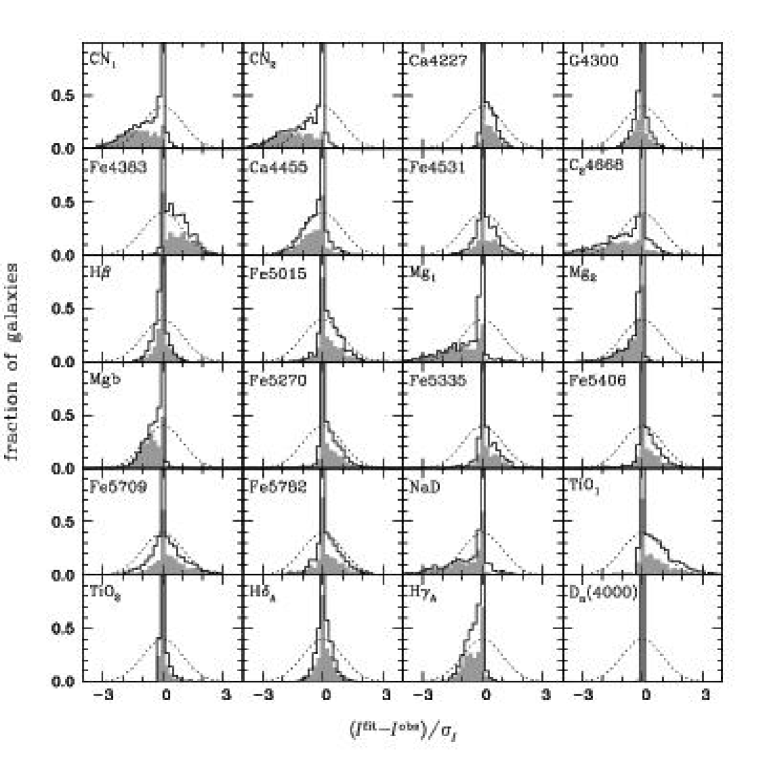
Figure 16: Fits of the strengths of individual indices in combination with $D_{n}(4000)$ in the spectra of 2010 galaxies with S/N${}_{\rm med}\geq 30$ in the ‘main galaxy sample’ of the SDSS EDR. The stellar velocity dispersion of the models are required to be within 15 ${\rm km}\,{\rm s}^{-1}$ of the observed ones. Each panel shows the distribution of the fitted index strength $I^{\rm fit}$ minus the observed one $I^{\rm obs}$, divided by the associated error $\sigma_{I}$ (equation 3). For reference, a dotted line in each panel indicates a Gaussian distribution with unit standard deviation. The shaded histograms show the contributions to the total distributions by galaxies with $\hbox{$\sigma_{V}$}>180~{}\hbox{${\rm km}\,{\rm s}^{-1}$}$, corresponding roughly to the median stellar velocity dispersion of the sample.

We can identify in Fig. 16 those Lick indices that our model fails to reproduce well when compared to high-quality galaxy spectra: CN₁, CN₂, C₂4668, Mg₁ and NaD. The distributions of $\left(I^{\rm fit}-I^{\rm obs}\right)/\sigma_{I}$ for these indices all show significant tails relative to a Gaussian distribution. These departures are most likely caused by differences in element abundance ratios between SDSS galaxies and the Galactic stars used to build our model. Several recent studies have addressed the influence of changes in element abundance ratios on the strengths of Lick indices (Tripicco & Bell 1995; Tantalo et al. 1998; Trager et al. 2000; Vazdekis et al. 2001; Proctor & Sansom 2002; Thomas, Maraston & Bender 2003). These studies were motivated by the observational evidence that the abundance ratios of $\alpha$-elements to iron are enhanced in massive early-type galaxies relative to the solar composition. The discrepancies found in these studies between models with scaled-solar abundances and observations of Lick indices in nearby star clusters and galaxies are similar to those identified above in Fig. 16. Enhanced abundances of Mg, C and N have been invoked to account for the departures of models from observations of CN₁, CN₂, C₂4668 and Mg₁. Some indices like NaD could also be contaminated by interstellar absorption. As Fig. 16 shows, the discrepancies pertaining to these indices tend to arise in galaxies with large velocity dispersions.

Our main goal here is to identify those indices that can be fitted by our model in observed galaxy spectra. Among the indices the model can recover within the errors at the same time as $D_{n}(4000)$ in Fig. 16, we expect a subset to also be reproducible simultaneously. In particular, since the Balmer-line indices H$\beta$, H$\gamma_{A}$ and H$\delta_{A}$ are not expected to depend sensitively on metallicity, they should also be reproducible in combination with metallic-line indices. We further expect our model to be able to reproduce metallic-line indices that do not depend sensitively on changes in $\alpha$-element to iron abundance ratios. The model with variable element abundance ratios of Thomas et al. (2003) is useful for identifying ‘composite’ indices that are sensitive to metallicity but not to $\alpha$/Fe. The original $\left[{\rm MgFe}\right]$ index of González (1993) and the new $\left[{\rm MgFe}\right]^{\prime}$ index proposed by Thomas et al. (2003), which is even less sensitive to $\alpha$/Fe, are both well calibrated in our model (see Fig. 18 below). After some experimentation, we identified two other indices with similarly weak dependence on $\alpha$/Fe,

$$\hbox{$\left[{\rm Mg}_{1}{\rm Fe}\right]$}=0.6{\rm Mg}_{1}+0.4\log({\rm Fe4531}+{\rm Fe5015})\,,$$ (4)

$$\hbox{$\left[{\rm Mg}_{2}{\rm Fe}\right]$}=0.6{\rm Mg}_{2}+0.4\log({\rm Fe4531}+{\rm Fe5015})\,.$$ (5)

Fig. 17 illustrates the evolution of $\left[{\rm MgFe}\right]^{\prime}$, $\left[{\rm Mg}_{1}{\rm Fe}\right]$ and $\left[{\rm Mg}_{2}{\rm Fe}\right]$ for SSPs with different metallicities, $\alpha$/Fe abundance ratios and stellar velocity dispersions. The left-hand panels show the predictions of the Thomas et al. (2003) model for the metallicities $Z=0.5Z_{\odot}$, $Z_{\odot}$ and $2.2Z_{\odot}$ and for [$\alpha$/Fe]= 0.0, 0.3 and 0.5, for a Salpeter (1955) IMF truncated at 0.1 and 100 $M_{\odot}$. The right-hand panels show the predictions of our model for the same IMF for the metallicities $Z=0.4Z_{\odot}$, $Z_{\odot}$ and $2.5Z_{\odot}$ and for stellar velocity dispersions $70\leq\hbox{$\sigma_{V}$}\leq 300\,\hbox{${\rm km}\,{\rm s}^{-1}$}$. It is clear from this figure that $\left[{\rm MgFe}\right]^{\prime}$, $\left[{\rm Mg}_{1}{\rm Fe}\right]$ and $\left[{\rm Mg}_{2}{\rm Fe}\right]$ are affected sensitively by changes in $Z$ and $\sigma_{V}$ but not by changes in $\alpha$/Fe. We note that, since Mg₁ and Mg₂ are defined over broader bandpasses than the Mgb index involved in the definition of $\left[{\rm MgFe}\right]^{\prime}$ (471 Å versus 64 Å), $\left[{\rm Mg}_{1}{\rm Fe}\right]$ and $\left[{\rm Mg}_{2}{\rm Fe}\right]$ may be slightly more sensitive to flux-calibration uncertainties and attenuation by dust in observed galaxy spectra.

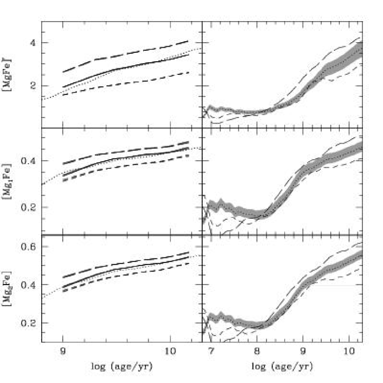
Figure 17: Left: Evolution of the strengths of $\left[{\rm MgFe}\right]^{\prime}$, $\left[{\rm Mg}_{1}{\rm Fe}\right]$ and $\left[{\rm Mg}_{2}{\rm Fe}\right]$ according to the model with variable element abundance ratios of Thomas et al. (2003) for the metallicities $Z=0.5Z_{\odot}$ (short-dashed lines), $Z_{\odot}$ (solid lines) and $2.2Z_{\odot}$ (long-dashed lines). For each metallicity, three lines corresponding to [$\alpha$/Fe]=0.0, 0.3 and 0.5 are shown (hardly distinguishable). The dotted line shows the evolution of an SSP with solar metallicity computed using the Padova 1994 stellar evolution prescription, the STELIB/BaSeL 3.1 spectral calibration and a Salpeter (1955) IMF (0.1–100 $M_{\odot}$), for a stellar velocity dispersion $\hbox{$\sigma_{V}$}=200~{}\hbox{${\rm km}\,{\rm s}^{-1}$}$. Right: Evolution of the strengths of $\left[{\rm MgFe}\right]^{\prime}$, $\left[{\rm Mg}_{1}{\rm Fe}\right]$ and $\left[{\rm Mg}_{2}{\rm Fe}\right]$ in SSPs computed using the Padova 1994 stellar evolution prescription, the STELIB/BaSeL 3.1 spectral calibration and a Salpeter (1955) IMF (0.1–100 $M_{\odot}$), for the metallicities $Z=0.4Z_{\sun}$ (short-dashed line), $Z_{\sun}$ (dotted line) and $2.5Z_{\sun}$ (long-dashed line) and for $\hbox{$\sigma_{V}$}=200~{}\hbox{${\rm km}\,{\rm s}^{-1}$}$. The shaded area around the solar-metallicity model indicates the range spanned by models with stellar velocity dispersions $70\leq\hbox{$\sigma_{V}$}\leq 300~{}\hbox{${\rm km}\,{\rm s}^{-1}$}$.

Based on these arguments, we use our library of models with different star formation histories to fit simultaneously the observed strengths of H$\beta$, H$\gamma_{A}$, H$\delta_{A}$, $\left[{\rm MgFe}\right]^{\prime}$, $\left[{\rm Mg}_{1}{\rm Fe}\right]$, $\left[{\rm Mg}_{2}{\rm Fe}\right]$ and $D_{n}(4000)$ in the 2010 SDSS spectra with S/N${}_{\rm med}>30$ in our sample. As before, for each SDSS spectrum, we select the best-fitting model in the library among those with stellar velocity dispersions within 15 ${\rm km}\,{\rm s}^{-1}$ of the observed one. Fig. 18 shows the resulting distributions of $\left(I^{\rm fit}-I^{\rm obs}\right)/\sigma_{I}$ for all galaxies in the sample, for the same 24 indices as in Fig. 16 and for $\left[{\rm MgFe}\right]$, $\left[{\rm MgFe}\right]^{\prime}$, $\left[{\rm Mg}_{1}{\rm Fe}\right]$ and $\left[{\rm Mg}_{2}{\rm Fe}\right]$. The highlighted frames indicate the seven indices used to constrain the fits. Fig. 18 demonstrates that our model can account simultaneously for the observed strengths of H$\beta$, H$\gamma_{A}$, H$\delta_{A}$, $\left[{\rm MgFe}\right]^{\prime}$, $\left[{\rm Mg}_{1}{\rm Fe}\right]$, $\left[{\rm Mg}_{2}{\rm Fe}\right]$ and $D_{n}(4000)$ in high-quality galaxy spectra. The strengths of these indices are always recovered within the errors. In addition, the model recovers reasonably well the strengths of several other indices which were not used to constrain the fits, such as G4300, Ca4455, Fe4531, Fe5015, Fe5270, Fe5335, Fe5709 and Fe5782. As expected from Fig. 16, indices like CN₁, CN₂, C₂4668, Mg₁ and NaD cannot be fitted accurately because of their strong dependence on element abundance ratios. The fact that Mgb appears to be better reproduced than Mg₁ and Mg₂ in Fig. 18 is a consequence of the larger relative error on this index (see Table 5). Interestingly, TiO₁ and TiO₂ that could be fitted individually in Fig. 16 do not appear to be well reproducible in combination with the other indices in Fig. 18.

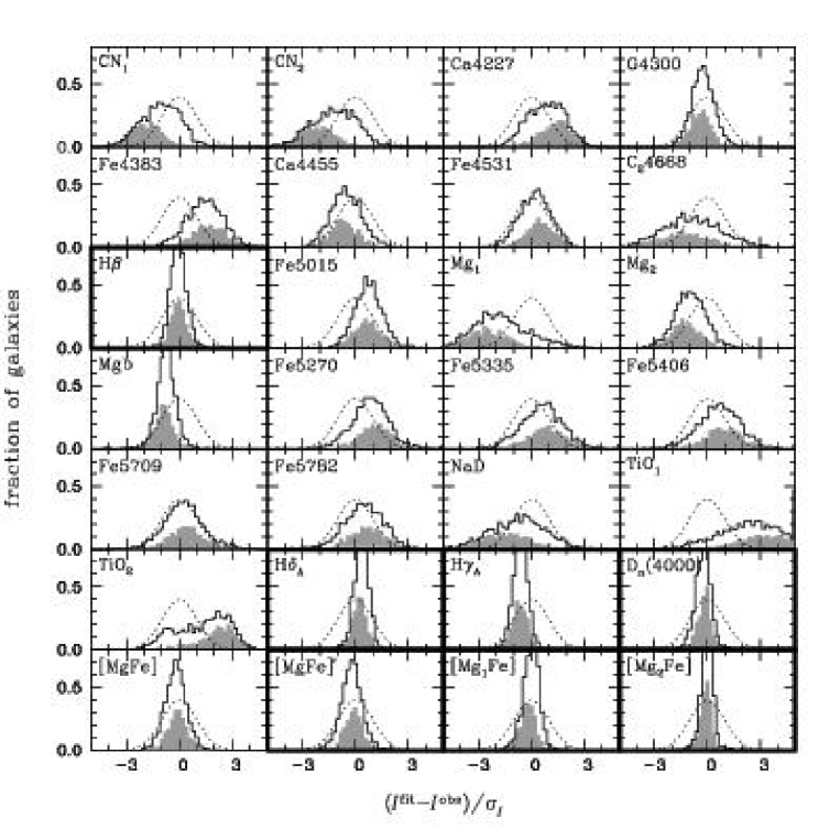
Figure 18: Simultaneous fit of the strengths of several indices in the spectra of 2010 galaxies with S/N${}_{\rm med}\geq 30$ in the ‘main galaxy sample’ of the SDSS EDR. The highlighted frames indicate the seven indices used to constrain the fits. The stellar velocity dispersion of the models are required to be within 15 ${\rm km}\,{\rm s}^{-1}$ of the observed ones. Each panel shows the distribution of the fitted index strength $I^{\rm fit}$ minus the observed one $I^{\rm obs}$, divided by the associated error $\sigma_{I}$ (equation 3). For reference, a dotted line in each panel indicates a Gaussian distribution with unit standard deviation. The shaded histograms show the contributions to the total distributions by galaxies with $\hbox{$\sigma_{V}$}>180~{}\hbox{${\rm km}\,{\rm s}^{-1}$}$, corresponding roughly to the median stellar velocity dispersion of the sample.

The agreement between model and observations for many indices in Fig. 18 is all the more remarkable in that the measurement errors for this sample of high-quality SDSS spectra are very small. As Table 5 shows, for indices such as H$\gamma_{A}$, H$\delta_{A}$, $D_{n}(4000)$, $\left[{\rm MgFe}\right]^{\prime}$, $\left[{\rm Mg}_{1}{\rm Fe}\right]$ and $\left[{\rm Mg}_{2}{\rm Fe}\right]$, the typical error $\overline{\sigma_{I}}$ amounts to only about 5–10 per cent of the total range spanned by the index over the full sample. Our model, therefore, represents an ideal tool for interpreting the distribution of these indices in complete samples of galaxies in terms of the parameters describing the stellar populations. Such analyses may include all types of galaxies, from star-forming galaxies to passively evolving, early-type galaxies, for which stellar velocity dispersions should first be determined.

4.4 Comparison with previous work

In most previous studies of absorption-line features in galaxy spectra, index strengths were computed in the Lick/image dissector scanner (IDS) system (see for example Worthey et al. 1994). To compare our results with these previous studies, we must therefore transform our predictions to the Lick/IDS system. This amounts to computing index strengths as if they were measured in spectra which are not flux-calibrated and whose resolution ranges from 8 Å to 10 Å FWHM, depending on wavelength. We follow the procedure outlined in the appendix of Worthey & Ottaviani (1997) and calibrate the transformation from STELIB to Lick/IDS spectra using 31 stars in common between the two libraries. We first broaden the STELIB spectra of these stars to the wavelength-dependent Lick/IDS resolution. Then, we identify the median offsets between the index strengths measured in the broadened STELIB spectra and those measured from the non-fluxed Lick/IDS spectra for the 31 stars. The resulting median offsets are listed in Table 6 for 25 spectral features. To compute predictions in the Lick/IDS system, therefore, we first broaden our model galaxy spectra to the Lick/IDS resolution and then subtract the median offsets of Table 6 from the index strengths measured in the broadened spectra.

Table 6: Median offsets in the strengths of 25 spectral features between the STELIB spectra broadened to the wavelength-dependent Lick/IDS resolution and the non-fluxed Lick/IDS spectra for the 31 stars in common between the two libraries. A positive offset denotes that the index measured from STELIB spectra is larger than that measured from Lick/IDS spectra. The values for atomic indices are expressed in angstroms of equivalent width, while those for molecular indices (indicated by a star) are expressed in magnitudes.

Feature	Median Offset
	(STELIB minus Lick/IDS)
⋆CN1	$-$0.011
⋆CN2	$-$0.001
Ca4227	$-$0.02
G4300	0.05
Fe4383	0.52
Ca4455	$-$0.13
Fe4531	$-$0.12
C24668	0.43
H$\beta$	0.13
Fe5015	0.47
⋆Mg1	$-$0.020
⋆Mg2	$-$0.018
Mgb	0.03
Fe5270	0.17
Fe5335	0.07
Fe5046	0.20
Fe5709	0.03
Fe5782	0.04
NaD	0.01
⋆TiO1	0.003
⋆TiO2	0.004
H$\delta_{A}$	0.83
H$\gamma_{A}$	$-$0.89
H$\delta_{F}$	0.20
H$\gamma_{F}$	$-$0.29

In Fig. 19, we compare different models for the evolution of the H$\delta_{A}$, Fe5270 and Mg₂ index strengths of a simple stellar population with solar composition ($Z=Z_{\odot}$, [$\alpha$/Fe] =0) and a Salpeter (1955) IMF. The left-hand panels show model predictions computed in the Lick/IDS system. The solid line shows our standard model transformed to the Lick/IDS system, as described above. Also shown, where available, are the models of Worthey (1994, dotted line), Vazdekis et al. (1996, long-dashed line), Worthey & Ottaviani (1997, dot-and-dashed line) and Thomas et al. (2003, short-dashed line). These models differ from ours in that they rely on the implementation of the ‘fitting formulae’ of Worthey et al. (1994) and Worthey & Ottaviani (1997) – who parametrized index strengths as functions of stellar effective temperature, gravity and metallicity (see Section 1 above) – into different population synthesis codes. The predictions are restricted to stellar populations older than 1 Gyr. As Fig. 19 shows, the strengths of H$\delta_{A}$, Fe5270 and Mg₂ predicted by our model when transformed to the Lick/IDS system are consistent with the predictions from these previous models to within the typical theoretical errors listed in Table 5.

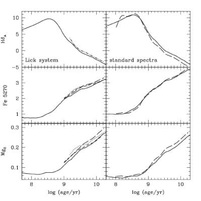
Figure 19: Evolution of the strengths of H$\delta_{A}$, Fe5270 and Mg₂ of an SSP with solar composition ($Z=Z_{\odot}$, [$\alpha$/Fe]=0) and a Salpeter (1955) IMF according to different models. Left: Predictions computed in the Lick/IDS system. In each panel, the solid line shows the standard model of Section 3 transformed to the Lick/IDS system, as described in the text. Also shown, where available, are the models of Worthey (1994, dotted line), Vazdekis et al. (1996, long-dashed line), Worthey & Ottaviani (1997, dot-and-dashed line) and Thomas et al. (2003, short-dashed line). Right: Index strengths measured in the same way in the spectra of the standard model of Section 3 (solid line) and in the spectra of the Vazdekis (1999) model broadened to a resolution of 3 Å FWHM (long-dashed line).

The recent model of Vazdekis (1999) offers another element of comparison, as it predicts the spectra of simple stellar populations of various ages and metallicities at a resolution of $\sim 1.8$ Å. Thus, the strengths of H$\delta_{A}$, Fe5270 and Mg₂ can be measured in these spectra in the same way as in our model, without having to transform predictions to the Lick/IDS system. In the right-hand panels of Fig. 19, we compare the strengths of H$\delta_{A}$, Fe5270 and Mg₂ in our model with those measured in the Vazdekis (1999) spectra broadened to a resolution of 3 Å FWHM, for an SSP with solar composition and a Salpeter (1955) IMF. The predictions of both models agree to within the typical theoretical errors listed in Table 5. As a further check, we compare in Fig. 20 the spectra predicted by both models for 10 Gyr-old SSPs with scaled-solar abundances, for the metallicities $0.4Z_{\sun}$ and $Z_{\sun}$. The spectra are shown in the two narrow wavelength regions covered by the Vazdekis (1999) model, 3820–4500 Å and 4780–5460 Å. The overall agreement between the two models is excellent at both metallicities. We conclude that our model agrees reasonably well with previous models of spectral indices of galaxies.

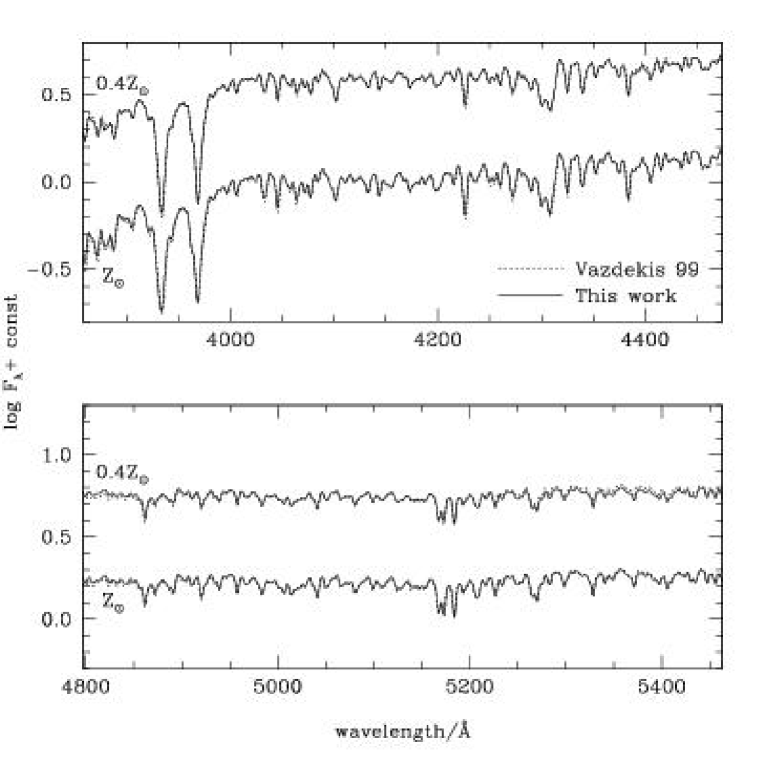
Figure 20: Comparison of the standard model of Section 3 (solid line) with the Vazdekis (1999) model broadened to a resolution of 3 Å FWHM (dotted line), for 10 Gyr-old SSPs with scaled-solar abundances and a Salpeter (1955) IMF, for the metallicities $0.4Z_{\sun}$ and $Z_{\sun}$. The spectra are shown in the two narrow wavelength regions covered by the Vazdekis (1999) model.

5 Summary and conclusions

We have presented a new model for computing the spectral evolution of stellar populations of different metallicities at ages between $1\times 10^{5}\,$yr and $2\times 10^{10}\,$yr at a resolution of 3 Å FWHM across the whole wavelength range from 3200 Å to 9500 Å (corresponding to a median resolving power $\lambda/\Delta\lambda\approx 2000$). These predictions are based on a new library of observed stellar spectra recently assembled by Le Borgne et al. (2003). The spectral evolution can also be computed across a larger wavelength range, from 91 Å to 160 $\mu$m, at lower resolution. The model incorporates recent progress in stellar evolution theory and an observationally motivated prescription for thermally-pulsing AGB stars, which is supported by observations of surface brightness fluctuations in nearby stellar populations (Liu et al. 2000; Liu et al. 2002). We have shown that this model reproduces well the observed optical and near-infrared colour-magnitude diagrams of Galactic star clusters of various ages and metallicities, and that stochastic fluctuations in the numbers of stars in different evolutionary phases can account for the full range of observed integrated colours of star clusters in the Magellanic Clouds and in the merger remnant galaxy NGC 7252.

Our model reproduces in detail typical galaxy spectra extracted from the SDSS Early Data Release (Stoughton et al., 2002). We have shown how this type of spectral fit can constrain physical parameters such as the star formation history, metallicity and dust content of galaxies. Our model is also the first to enable accurate studies of absorption-line strengths in galaxies containing stars over the full range of ages. We have shown that it can reproduce simultaneously the observed strengths of those Lick indices that do not depend strongly on element abundance ratios in 2010 spectra with S/N${}_{\rm med}\geq 30$, taken from the ‘main galaxy sample’ of the SDSS EDR. This comparison requires proper accounting for the observed velocity dispersions of the galaxies. Indices whose strengths depend strongly on element abundance ratios cannot always be fitted accurately, because the stars in the model spectral library have fixed composition at fixed metallicity. Based on the model with variable element abundance ratios of Thomas et al. (2003), we have identified a few spectral features which depend negligibly on element abundance ratios and are well reproduced by our model: $\left[{\rm MgFe}\right]^{\prime}$, $\left[{\rm Mg}_{1}{\rm Fe}\right]$ and $\left[{\rm Mg}_{2}{\rm Fe}\right]$ (equations 4–5). These features, when combined with a Balmer-line index such as H$\beta$, H$\gamma_{A}$ or H$\delta_{A}$, should be particularly useful for constraining the star formation histories and metallicities of galaxies. Several other popular indices, such as the Ca II triplet index near 8500 Å (Díaz et al., 1989), can also be measured directly from the model spectra. Most interestingly, our model offers the possibility to explore new indices over the full wavelength range from 3200 Å to 9500 Å.

It is worth mentioning that, for applications to studies of star-forming galaxies, the influence of the interstellar medium on the stellar radiation predicted by our model must be accounted for. The emission-line spectrum of the H ii regions and the diffuse gas ionized by young stars can be computed by combining our model with a standard photoionization code (see for example Charlot & Longhetti 2001). To account for the attenuation of starlight by dust, the simple but realistic prescription of Charlot & Fall (2000) is particularly well suited to population synthesis studies. In this prescription, the attenuation of starlight by dust may be accounted for by inserting a factor $\exp[-\hat{\tau}_{\lambda}(t^{\prime})]$ in the integrand on the right-hand side of equation (1), where $\hat{\tau}_{\lambda}(t^{\prime})$ is the ‘effective absorption’ curve describing the attenuation of photons emitted in all directions by stars of age $t^{\prime}$ in a galaxy. This is given by the simple formula

$$\hat{\tau}_{\lambda}(t^{\prime})=\cases{\hskip 6.25963pt\hat{\tau}_{V}\left(\lambda/{5500\,\mathrm{\AA}}\right)^{-0.7}\,,&for $t^{\prime}\leq 10^{7}$ yr,\cr{{\mu\hat{\tau}_{V}}}\left(\lambda/{5500\,\mathrm{\AA}}\right)^{-0.7}\,,&for $t^{\prime}>10^{7}$ yr,\cr}$$ (6)

where $\hat{\tau}_{V}$ is the total effective $V$-band optical depth seen by young stars. The characteristic age $10^{7}\,$yr corresponds to the typical lifetime of a giant molecular cloud. The adjustable parameter $\mu$ defines the fraction of the total dust absorption optical depth of the galaxy contributed by the diffuse interstellar medium ($\mu\approx 1/3$ on average, with substantial scatter). Note that equation (6) neglects the absorption of ionizing photons by dust in the H ii regions, that should be accounted for to study line luminosities (see Charlot et al. 2002).

The high-resolution population synthesis model presented in this paper enables more refined spectral analyses of galaxies than could be achieved using previous low-resolution models. In particular, in recent studies of our own, it has become clear that the ability to resolve stellar absorption features in galaxy spectra demonstrates a need in many galaxies to account for the stochastic nature of star formation (e.g., Kauffmann et al. 2003; see also Section 4.3 above). Traditional models with continuous star formation histories tend to smooth away valuable spectral signatures of stochastic starbursts. Our preliminary results also suggest that the new high-resolution model makes it possible to break, in many cases, the age-metallicity degeneracy which has impaired most previous population synthesis studies of the star formation and enrichment histories of galaxies. We hope that this model will contribute to the refinement of such studies in the future. Our model is intended for use by the general astronomical community and is available from http://www.cida.ve/$\sim$bruzual/bc2003 and http://www.iap.fr/$\sim$charlot/bc2003.

Appendix A Mapping of theoretical isochrones with stellar spectra

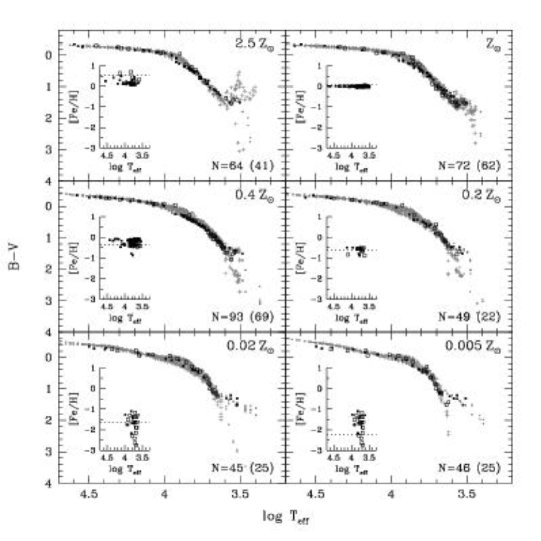
Figure 21: $B\!-\!V$ colour as a function of effective temperature for those stars of the BaSeL 3.1 (grey dots: dwarfs; grey crosses: giants) and STELIB/BaSeL 3.1 (black filled squares: dwarfs; black open squares: giants) libraries that were selected to map the theoretical isochrones computed using the Padova 1994 evolutionary tracks, as described in Appendix A. Each panel corresponds to a different metallicity of the evolutionary tracks, as indicated. For each metallicity, the inset panel shows [Fe/H] as a function of $\log T_{\rm eff}$ for the subset of STELIB stars included in the metallicity bin whose abundances are compatible with the [Fe/H] value of the evolutionary tracks (indicated by a dotted line). The number of these stars is given in parentheses at the bottom right of each panel. Also indicated is the total number N of STELIB stars included in the metallicity bin and shown on the colour-temperature relation. This number includes, in addition to the stars shown in the inset panel, cool K- and M-dwarf stars from the SDSS EDR (whose colours are taken to be the same at all metallicities) and hot solar-metallicity stars (see text for detail).

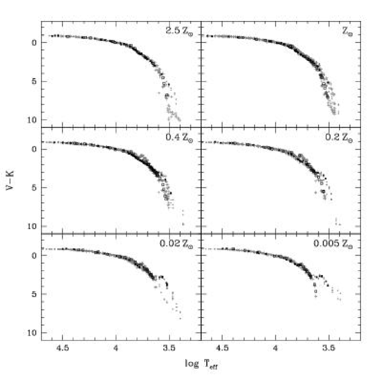
Figure 22: $V\!-\!K$ colour as a function of effective temperature for those stars of the BaSeL 3.1 (grey dots: dwarfs; grey crosses: giants) and STELIB/BaSeL 3.1 (black filled squares: dwarfs; black open squares: giants) libraries that were selected to map the theoretical isochrones computed using the Padova 1994 evolutionary tracks, as described in Appendix A. Each panel corresponds to a different metallicity of the evolutionary tracks, as indicated.

We illustrate here in a graphical way the mapping of theoretical isochrones with stellar spectra in our model. At fixed metallicity $Z$ (or [Fe/H]), an isochrone interpolated from a set of stellar evolutionary tracks in the HR diagram is defined by a sequence of evolutionary phases corresponding to different effective temperatures $\log T_{\rm eff}$ and gravities $\log g$. To transform this theoretical isochrone into an observational one, we must assign a stellar spectrum to each of the evolutionary phases. This is straightforward in the case where the spectra are taken from a library of theoretical model atmospheres (i.e., BaSeL 1.0, BaSeL 2.2, BaSeL 3.1; see Tables 2 and 3), since in general such models are parametrized in terms of $Z$, $\log T_{\rm eff}$ and $\log g$. The only practical complication in this case is that model atmospheres are available only for discrete values of these parameters. Thus model spectra must be interpolated at the values of $Z$, $\log T_{\rm eff}$ and $\log g$ corresponding to the isochrone. The relation between colours and effective temperature for stars of fixed metallicity and gravity is then tied to the adopted spectral library (Section 2.2.1).

We now turn to the case where the STELIB library of observed stellar spectra is used to map the theoretical isochrones in the HR diagram. In this case, we still rely on the colour-temperature scale of one of the BaSeL libraries in Table 3. The reason for this is that the effective temperatures published by Le Borgne et al. (2003) for the STELIB stars are incomplete and were not derived in a homogeneous way. Hence these temperatures are not suited to model calibration. We therefore assign to each evolutionary stage along the isochrone the STELIB spectrum of the corresponding luminosity class that best matches the theoretical BaSeL spectrum assigned to that stage. In this procedure, the STELIB spectra are first degraded to the resolution of the BaSeL library using a gaussian filter of 20 Å FWHM. The selection is thus driven by the shape of the continuum spectrum rather than by the strengths of absorption features (we have checked that this approach is free of systematic biases). We refer to the three possible implementations of the STELIB library in our model as the ‘STELIB/BaSeL 1.0’, the ‘STELIB/BaSeL 2.2’ and the ‘STELIB/BaSeL 3.1’ libraries (Section 2.2.2).

Figs. 21 and 22 show the $B\!-\!V$ and $V\!-\!K$ colours of those stars of the BaSeL 3.1 and STELIB/BaSeL 3.1 libraries that were selected as described above to map the theoretical isochrones computed using the Padova 1994 evolutionary tracks, for different metallicities. The colours are plotted as a function of effective temperature $T_{\rm eff}$, and different symbols represent dwarf and giant stars in each library. In the case of the STELIB/BaSeL 3.1 library, the $B\!-\!V$ colours rely on the STELIB spectra alone, while the $V\!-\!K$ colours rely on extensions of these spectra at near-infrared wavelengths using BaSeL 3.1 spectra (Section 2.2.2).

By construction, at fixed metallicity, the colour-temperature scale of the STELIB/BaSeL 3.1 library is always similar to that of the BaSeL 3.1 library. The number of STELIB stars with metallicities close to that of the evolutionary tracks is indicated in parentheses at the bottom right of each panel in Fig. 21. The inset panels in Fig. 21 show [Fe/H] as a function of $\log T_{\rm eff}$ for these stars. Because of the scarcity of stars hotter than about 7000 K at non-solar metallicities, we include hot solar-metallicity stars to sample the colour-$T_{\rm eff}$ relations at all metallicities. As mentioned in Section 2.2.1, the spectra of these stars should be representative of hot stars at all but the most extreme metallicities. For completeness, we also include in the STELIB library a few SDSS-EDR spectra of cool K- and M-dwarf stars at all metallicities (we thank C. Tremonti for kindly providing us with these spectra). For standard IMFs, these stars never contribute significantly to the integrated light of model stellar populations. The total number of STELIB stars used to sample the colour-temperature relation at each metallicity (including hot solar-metallicity stars and SDSS-EDR cool dwarf stars) is indicated at the bottom right of each panel in Fig. 21.

Table 7: Qualitative assessment of the spectral predictions of the model for simple stellar populations of various ages and metallicities computed using the Padova 1994 evolutionary tracks and different spectral libraries. For each entry, the expected reliability of the predictions is indicated separately for young ($\la 1\,$Gyr) and old ($\gg 1\,$Gyr) stellar populations (listed as young/old).

Metallicity	STELIB/BaSeL 3.1		BaSeL 3.1	Pickles
(Padova 1994)	optical colours	line strengths	UV–NIR colours	UV–NIR colours
$2.5\,Z_{\odot}$	good/good	fair/faira	fair/poor	…
$Z_{\odot}$	very good/very good	very good/very good	very good/good	very good/very good
$0.4\,Z_{\odot}$	good/good	good/very good	good/fair	…
$0.2\,Z_{\odot}$	fair/good	fair/good	good/fair	…
$0.02\,Z_{\odot}$	poor/fair	poor/fair	fair/poor	…
$0.005\,Z_{\odot}$	poor/fair	poor/fair	poor/poor	…

${}^{a}\,$The STELIB spectra used to map the theoretical isochrones have $\hbox{\rm[Fe/H]}\approx+0.25$ on average, i.e., slightly lower than the metallicity of the evolutionary tracks (Fig. 21). This affects line strengths but not colour predictions, which are tied to the colour-temperature scale of the BaSeL 3.1 library for $Z=2.5\,Z_{\odot}$.

Figs. 21 and 22 allow us to draw the following conclusions. First, the STELIB spectra of dwarf and giant stars used to sample the colour-$T_{\rm eff}$ relation in each metallicity bin provide reasonable coverage of the HR diagram. In practice, in regions where the sampling is scarcer (for example, around $\mbox{$B\!-\!V$}\approx 0.1$ and $\log T_{\rm eff}\approx 3.9$ at the metallicity $0.4\,Z_{\sun}$ in Fig. 21), we improve it by interpolating between nearby STELIB spectra of the appropriate luminosity class. We do not perform such interpolations in the temperature range 3750–5000 K that is critical for bright giant stars and is always well sampled. Second, the homogeneity in [Fe/H] of STELIB stars included in each metallicity bin varies from bin to bin. It is reasonable for $Z\geq 0.4Z_{\sun}$, although we note that for $Z=2.5Z_{\sun}$ the STELIB stars have $\hbox{\rm[Fe/H]}\approx+0.25$ on average, i.e., slightly lower metallicity than the tracks. There are no stars at all hotter than 7000 K at metallicities $Z\leq 0.2Z_{\sun}$. At these metallicities, the model relies heavily on our adoption of solar-metallicity spectra at high temperatures. Third, both Figs. 21 and 22 show that the STELIB library does not include giant stars as red as the reddest stars selected from the BaSeL 3.1 library to map the theoretical isochrones, even at solar metallicity. These stars, however, do not contribute critically to the integrated light of model stellar populations for standard IMFs. This is illustrated by the close agreement between the dotted (BaSeL 3.1) and solid (STELIB/BaSeL 3.1) lines in Fig. 3. It is worth recalling that, for the brightest asymptotic-giant-branch stars, we adopt in all libraries the prescription outlined in Section 2.2.4 (these stars have redder colours off the scales of Figs. 21 and 22).

We have performed further extensive tests of the $UBVRIJHKL$ colour-temperature scales, colour-colour relations and bolometric corrections of the different spectral libraries used in our model (Table 2). We find that our procedure to assign spectra from these libraries to stars in the HR diagram does not introduce any systematic bias in the predicted photometric evolution of stellar populations. The libraries themselves, however, include their own uncertainties. In particular, the ultraviolet and near-infrared colours of the spectra, even in the most recent BaSeL 3.1 library, remain significantly more uncertain than the optical colours because in part of the lack of comparison standards at non-solar metallicities (Westera et al., 2002). The situation should improve as more observed spectra become available to extend the optical spectra at ultraviolet and near-infrared wavelengths, as is the case already for solar metallicity (Pickles library). We further conclude that, despite the limitations outlined above, the STELIB library provides reasonable coverage of the HR diagram for population synthesis purposes, especially at metallicities greater than $0.2Z_{\odot}$. Based on these arguments, we can assess the expected accuracy of the spectral predictions of our model for simple stellar populations of various ages and metallicities computed using the Padova 1994 evolutionary tracks and different spectral libraries. This qualitative assessment is summarized in Table 7.

References

- Alexander & Ferguson (1994) Alexander, D. R., Ferguson, J. W. 1994, ApJ, 437, 879